

Nuclear Energy 5.0: New Formation and System Architecture of Nuclear Power Industry in the New IT Era
-
摘要: 本文旨在讨论核能5.0(Nuclear Energy 5.0)的基本概念、体系架构和关键平台技术等问题.首先讨论了核能5.0出现的新智能时代基础,阐述了虚拟数字工业崛起的技术背景.详细叙述了核电工业新形态与体系结构,即平行核能的定义、意义、研究内容、体系架构以及应用领域.接下来讨论了核能5.0中新一代核心技术,包括核能物联网、知识自动化、发展性人工智能、大规模协同演进技术、核能区块链等.最后讨论了核能5.0中在核电系统的具体应用场景与案例,重点是核电工控系统安全评估与核电站数字化仪控系统.Abstract: This paper aims to provide a blueprint for Nuclear Energy 5.0 (NE 5.0), discussing its concept, system architecture and platform technology. We start with a discussion on the social foundation for NE 5.0. Then we illustrate the background of NE 5.0's emergence, which is the rise of virtual digital industry together with its definition, essence, contents, system architecture and application areas. Next we discuss the novel platform technology of NE 5.0 including internet of minds, knowledge automation, developmental artificial intelligence, large-scale co-evolutionary techniques, industrial blockchain, etc. Finally we present two application case studies of NE 5.0 in nuclear power system, i.e., security assessment of nuclear power plant control system and nuclear power plant digital I & C system.
-
Key words:
- Nuclear energy /
- internet of minds /
- knowledge automation /
- parallel system /
- ACP approach /
- blockchain /
- virtual digital industry
1) 本文责任编委 刘德荣 -

图 8 核电工控系统信息安全保障方案平台评估流程
Fig. 8 Nuclear power information security program platform for industrial control systems assessment process
图 9 核电工控系统信息安全计算实验图例
Fig. 9 Nuclear power control system of information security computing experiments instance
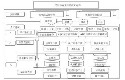
图 10 基于平行理论的核电仪控技术研究架构
Fig. 10 Parallel instrumentation and control system structure of nuclear power
-
[1] 张廷克, 李闽榕, 潘启龙.中国核能发展报告(2018).北京:社会科学文献出版社, 2018. [2] 卡尔·波普尔.客观知识:一个进化论的研究.上海:上海译文出版社, 1972.Popper K R. Objective Knowledge:An Evolutionary Approach. Shanghai:Shanghai Translation Publishing House, 1972. [3] Jaspers K. The Origin and Goal of History. Munich:Piper Verlag GmbH, 1949. [4] 库尔特·哥德尔. 〈数学原理〉及有关系统中的形式不可判定命题. 1931.Gödel K. On Formally Undecidable Propositions of Principia Mathematica and Related Systems(Ⅰ). 1931. [5] 王飞跃.软件定义的系统与知识自动化:从牛顿到默顿的平行升华.自动化学报, 2015, 41(1):1-8 http://www.aas.net.cn/CN/abstract/abstract18578.shtmlWang Fei-Yue. Software-defined systems and knowledge automation:a parallel paradigm shift from Newton to Merton. Acta Automatica Sinica, 2015, 41(1):1-8 http://www.aas.net.cn/CN/abstract/abstract18578.shtml [6] Wang F Y. The emergence of intelligent enterprises:from CPS to CPSS. IEEE Intelligent Systems, 2010, 25(4):85-88 doi: 10.1109/MIS.2010.104 [7] 王飞跃, 杨坚, 韩双双, 杨柳青, 程翔.基于平行系统理论的平行网络架构.指挥与控制学报, 2016, 2(1):71-77 https://www.researchgate.net/profile/Fei_Yue_Wang/publication/317328968_The_Framework_of_Parallel_Network_Based_on_the_Parallel_System_Theory/links/5932737845851553b6aabedf/The-Framework-of-Parallel-Network-Based-on-the-Parallel-System-Theory.pdfWang Fei-Yue, Yang Jian, Han Shuang-Shuang, Yang Liu-Qing, Cheng Xiang. The framework of parallel network based on the parallel system theory. Journal of Command and Control, 2016, 2(1):71-77 https://www.researchgate.net/profile/Fei_Yue_Wang/publication/317328968_The_Framework_of_Parallel_Network_Based_on_the_Parallel_System_Theory/links/5932737845851553b6aabedf/The-Framework-of-Parallel-Network-Based-on-the-Parallel-System-Theory.pdf [8] 王飞跃. X5. 0: 平行时代的平行智能体系. 新时代智能论坛, 2015. https://www.researchgate.net/publication/317328952_X50pingxingshidaidepingxingzhinengtixiWANG Fei-Yue. X5. 0: Parallel Intelligence System in Parallel ERA. The New Intelligence Age Forum. 2015. https://www.researchgate.net/publication/317328952_X50pingxingshidaidepingxingzhinengtixi [9] 王飞跃.平行系统方法与复杂系统的管理和控制.控制与决策, 2004, 19(5):485-489 http://mall.cnki.net/magazine/Article/KZYC200405001.htmWang Fei-Yue. Parallel system methods for management and control of complex systems. Control and Decision, 2004, 19(5):485-489 http://mall.cnki.net/magazine/Article/KZYC200405001.htm [10] 王飞跃.平行控制:数据驱动的计算控制方法.自动化学报, 2013, 39(4):293-302 http://www.aas.net.cn/CN/abstract/abstract17915.shtmlWang Fei-Yue. Parallel control:a method for data-driven and computational control. Acta Automatica Sinica, 2013, 39(4):293-302 http://www.aas.net.cn/CN/abstract/abstract17915.shtml [11] 宁滨, 王飞跃, 董海荣, 文丁.高速铁路平行控制与管理系统研究框架.复杂系统与复杂性科学, 2010, 7(4):11-21 http://www.wanfangdata.com.cn/details/detail.do?_type=perio&id=fzxtyfzxkx201004002Ning Bin, Wang Fei-yue, Dong Hai-rong, Wen Ding. Framework of parallel control and management for high-speed railway systems. Complex Systems And Complexity Science, 2010, 7(4):11-21 http://www.wanfangdata.com.cn/details/detail.do?_type=perio&id=fzxtyfzxkx201004002 [12] Glaessgen E H, Stargel D S. The digital twin paradigm for future NASA and U. S. air force vehicles. In: Proceedings of the 53rd AIAA/ASME/ASCE/AHS/ASC Structures, Structural Dynamics and Materials Conference. Honolulu, Hawaii, USA: AIAA, 2012. doi: 10.2514/6.2012-1818 [13] Weber A. GE 'predix' the future of manufacturing. Assembly, 2017, 60(3):GE70-GE76 https://www.ptc.com/en/news/2016/ptc-and-ge-digital-to-expand-strategic-alliance [14] 熊刚, 董西松, 王兆魁, 王飞跃. 平行控制与管理的研究及应用进展综述. 中国空天安全会议, 2017 http://cpfd.cnki.com.cn/Article/CPFDTOTAL-ZHKT201708001090.htmXiong Gang, Dong Xi-Song, Wang Zhao-Kui, Wang Fei-Yue. Research and Application Review of Parallel Control and Management. Chinese Aerospace Safety Symposium, 2017 http://cpfd.cnki.com.cn/Article/CPFDTOTAL-ZHKT201708001090.htm [15] 王飞跃. 复杂系统的控制与管理机制研究及其应用. 见: 中国科学院院长基金特别支持项目立项书. 北京, 2005.Wang Fei-Yue. New mechanisms for control and management of complex systems: research and development. In: Project to the Presidents Foundation for Special Projects, Chinese Academy of Sciences. Beijing, China, 2005. [16] Wang F Y, Wang X, Li L X, Li L. Steps toward parallel intelligence. IEEE/CAA Journal of Automatica Sinica, 2016, 3(4):345-348 doi: 10.1109/JAS.2016.7510067 [17] 李力, 林懿伦, 曹东璞, 郑南宁, 王飞跃.平行学习——机器学习的一个新型理论框架.自动化学报, 2017, 43(1):1-8 http://www.aas.net.cn/CN/abstract/abstract18984.shtmlLi Li, Lin Yi-Lun, Cao Dong-Pu, Zheng Nan-Ning, Wang Fei-Yue. Parallel learning:a new framework for machine learning. Acta Automatica Sinica, 2017, 43(1):1-8 http://www.aas.net.cn/CN/abstract/abstract18984.shtml [18] Wang F Y, Zhang J, Wei Q L, Zheng X H, Li L. PDP:parallel dynamic programming. IEEE/CAA Journal of Automatica Sinica, 2017, 4(1):1-5 doi: 10.1109/JAS.2017.7510310 [19] 王飞跃, 王晓, 袁勇, 王涛, 林懿伦.社会计算与计算社会:智慧社会的基础与必然.科学通报, 2015, 60(5-6):460-469 http://mall.cnki.net/magazine/Article/KXTB2015Z1008.htmWang Fei-Yue, Wang Xiao, Yuan Yong, Wang Tao, Lin Yi-Lun. Social computing and computational societies:the foundation and consequence of smart societies. Chinese Science Bulletin, 2015, 60(5-6):460-469 http://mall.cnki.net/magazine/Article/KXTB2015Z1008.htm [20] Wang F Y, Wong P K. Intelligent systems and technology for integrative and predictive medicine:an ACP approach. ACM Transactions on Intelligent Systems and Technology, 2013, 4(2):Article No.32 http://europepmc.org/abstract/med/24883228 [21] Wang F Y. Toward a paradigm shift in social computing:the ACP approach. IEEE Intelligent Systems, 2007, 22(5):65-67 doi: 10.1109/MIS.2007.4338496 [22] Wang F Y. Parallel control and management for intelligent transportation systems:concepts, architectures, and applications. IEEE Transactions on Intelligent Transportation Systems, 2010, 11(3):630-638 doi: 10.1109/TITS.2010.2060218 [23] 王飞跃, 李晓晨, 毛文吉, 王涛.社会计算的基本方法与应用.杭州:浙江大学出版社, 2012.Wang Fei-Yue, Li Xiao-Chen, Mao Wen-Ji, Wang Tao. Social Computing:Methods and Applications. Hangzhou:Zhejiang University Press, 2012. [24] 王飞跃. 社会能源与平行能源系统: 迈向能源5. 0的时代. 见: 分布式能源专业委员会筹备会及IEEE ITSS北京分会. 北京: 北方工业大学, 2015.Wang Fei-Yue. Social energy and parallel energy systems: towards the age of energy 5. 0. In: Workshop on Distributed Energy Systems and Annual Symposium of IEEE ITSS Beijing Chapter. Beijing, China: North China University of Technology, 2015. [25] 王飞跃, 赵杰, 伦淑娴.人工电力系统与复杂大电网的运营和管理.南方电网技术, 2008, 2(3):1-6 http://www.cqvip.com/QK/88821X/200803/27981370.htmlWang Fei-Yue, Zhao Jie, Lun Shu-Xian. Artificial power systems for the operation and management of complex power grids. Southern Power System Technology, 2008, 2(3):1-6 http://www.cqvip.com/QK/88821X/200803/27981370.html [26] 赵俊华, 文福拴, 薛禹胜, 董朝阳.电力信息物理融合系统的建模分析与控制研究框架.电力系统自动化, 2011, 35(16):1-8 http://mall.cnki.net/magazine/Article/DLXT201116000.htmZhao Jun-Hua, Wen Fu-Shuan, Xue Yu-Sheng, Dong Zhao-Yang. Modeling analysis and control research framework of cyber physical power systems. Automation of Electric Power Systems, 2011, 35(16):1-8 http://mall.cnki.net/magazine/Article/DLXT201116000.htm [27] 赵俊华, 文福拴, 薛禹胜, 李雪, 董朝阳.电力CPS的架构及其实现技术与挑战.电力系统自动化, 2010, 34(16):1-7 http://mall.cnki.net/magazine/article/DLXT201016000.htmZhao Jun-Hua, Wen Fu-Shuan, Xue Yu-Sheng, Li Xue, Dong Zhao-Yang. Cyber physical power systems:architecture, implementation techniques and challenges. Automation of Electric Power Systems, 2010, 34(16):1-7 http://mall.cnki.net/magazine/article/DLXT201016000.htm [28] Ilic M D, Xie L, Khan U A, Moura J M F. Modeling of future cyber-physical energy systems for distributed sensing and control. IEEE Transactions on Systems, Man, and Cybernetics. Part A:Systems and Humans, 2010, 40(4):825-838 doi: 10.1109/TSMCA.2010.2048026 [29] Xie L, Ilic M D. Module-based modeling of cyber-physical power systems. In: Proceedings of the 28th International Conference on Distributed Computing Systems Workshops. Beijing, China: IEEE, 2008. 513-518 http://dl.acm.org/citation.cfm?id=1439719 [30] McMillin B. Complexities of information security in cyber-physical power systems. In: Proceedings of the 2009 IEEE/PES Power Systems Conference and Exposition. Seattle, WA, USA: IEEE, 2009. 1-2 http://ieeexplore.ieee.org/document/4840093/ [31] Singh C, Sprintson A. Reliability assurance of cyber-physical power systems. In: Proceedings of the 2010 IEEE Power and Energy Society General Meeting. Minneapolis, MN, USA: IEEE, 2010. 1-6 http://www.researchgate.net/publication/224179251_Reliability_assurance_of_cyber-physical_power_systems [32] 邓建玲, 王飞跃, 陈耀斌, 赵向阳.从工业4.0到能源5.0:智能能源系统的概念、内涵及体系框架.自动化学报, 2015, 41(12):2003-2016 http://www.aas.net.cn/CN/abstract/abstract18774.shtmlDeng Jian-Ling, Wang Fei-Yue, Chen Yao-Bin, Zhao Xiang-Yang. From industries 4.0 to energy 5.0:concept and framework of intelligent energy systems. Acta Automatica Sinica, 2015, 41(12):2003-2016 http://www.aas.net.cn/CN/abstract/abstract18774.shtml [33] 王飞跃.指控5.0:平行时代的智能指挥与控制体系.指挥与控制学报, 2015, 1(1):107-120 http://www.wanfangdata.com.cn/details/detail.do?_type=perio&id=zhykzxb201501018Wang Fei-Yue. CC 5.0:intelligent command and control systems in the parallel age. Journal of Command and Control, 2015, 1(1):107-120 http://www.wanfangdata.com.cn/details/detail.do?_type=perio&id=zhykzxb201501018 [34] 江泽民.对中国能源问题的思考.上海交通大学学报, 2008, 42(3):345-359 http://mall.cnki.net/magazine/Article/SHJT200803002.htmJiang Ze-Min. Reflections on energy issues in China. Journal of Shanghai Jiaotong University, 2008, 42(3):345-359 http://mall.cnki.net/magazine/Article/SHJT200803002.htm [35] 张力. 概率安全评价中人因可靠性分析技术研究[博士学位论文], 湖南大学, 中国, 2004 http://cdmd.cnki.com.cn/Article/CDMD-10532-2005040162.htmZhang Li. The Research on Human Reliability Analysis Technique in Probabilistic Safety Assessment[Ph. D. dissertation], Hu'nan University, China, 2004 http://cdmd.cnki.com.cn/Article/CDMD-10532-2005040162.htm [36] 薛禹胜, 肖世杰.综合防御高风险的小概率事件:对日本相继天灾引发大停电及核泄漏事件的思考.电力系统自动化, 2011, 35(8):1-11 http://industry.wanfangdata.com.cn/dl/Detail/Periodical?id=Periodical_dlxtzdh201108001Xue Yu-Sheng, Xiao Shi-Jie. Comprehensively defending high risk events with low probability. Automation of Electric Power Systems, 2011, 35(8):1-11 http://industry.wanfangdata.com.cn/dl/Detail/Periodical?id=Periodical_dlxtzdh201108001 [37] 荆春宁, 赵科, 张力友, 李辉, 王诚诚, 钱怡洁, 等. "华龙一号"的设计理念与总体技术特征.中国核电, 2017, 10(4):463-467 http://www.cqvip.com/QK/89379X/201302/46329432.htmlJing Chun-Ning, Zhao Ke, Zhang Li-You, Li Hui, Wang Cheng-Cheng, Qian Yi-Jie, et al. The design philosophy and general technical features of HPR1000. China Nuclear Power, 2017, 10(4):463-467 http://www.cqvip.com/QK/89379X/201302/46329432.html [38] 朱正威, 王琼, 吕书鹏.多元主体风险感知与社会冲突差异性研究——基于Z核电项目的实证考察.公共管理学报, 2016, (2):97-106 http://www.cqvip.com/QK/87267X/201602/668566259.htmlZhu Zheng-Wei, Wang Qiong, Lv Shu-Peng. Research on differences of multiple stakeholders' risk perception and social conflict——Empirical investigation of Z nuclear power project. Journal of Public Management, 2016, (2):97-106 http://www.cqvip.com/QK/87267X/201602/668566259.html [39] 李鹏程, 张力, 戴立操, 邹衍华, 青涛, 胡鸿等.核电厂数字化主控室操纵员的情景意识可靠性模型.系统工程理论与实践, 2016, 36(1):243-252 doi: 10.12011/1000-6788(2016)01-0243-10Li Peng-Cheng, Zhang Li, Dai Li-Cao, Zou Yan-Hua, Qing Tao, Hu Hong, et al. Operator's situation awareness reliability model in digital main control rooms of nuclear power plants. Systems Engineering——Theory and Practice, 2016, 36(1):243-252 doi: 10.12011/1000-6788(2016)01-0243-10 [40] 王晓磊, 吕大刚.核电厂地震概率风险评估研究综述.土木工程学报, 2016, 49(11):52-68 http://www.cnki.com.cn/Article/CJFDTotal-DEFE201206003.htmWang Xiao-Lei, Lv Da-Gang. Review of seismic probability risk assessment of nuclear power plants. China Civil Engineering Journal, 2016, 49(11):52-68 http://www.cnki.com.cn/Article/CJFDTotal-DEFE201206003.htm [41] 苏罡.中国核能科技"三步走"发展战略的思考.科技导报, 2016, 34(15):33-41 http://blog.sciencenet.cn/blog-336909-1005353.htmlSu Gang. The "three steps development strategy" of China nuclear power science and technology. Science & Technology Review, 2016, 34(15):33-41 http://blog.sciencenet.cn/blog-336909-1005353.html [42] 王飞跃, 张俊.智联网:概念、问题和平台.自动化学报, 2017, 43(12):2061-2070 http://www.aas.net.cn/CN/abstract/abstract19181.shtmlWang Fei-Yue, Zhang Jun. Internet of minds:the concept, issues and platforms. Acta Automatica Sinica, 2017, 43(12):2061-2070 http://www.aas.net.cn/CN/abstract/abstract19181.shtml [43] 程乐峰, 余涛, 张孝顺, 殷林飞, 瞿凯平.信息-物理-社会融合的智慧能源调度机器人及其知识自动化:框架、技术与挑战.中国电机工程学报, 2018, 38(1):25-40 http://www.cnki.com.cn/Article/CJFDTotal-DLXT201415001.htmCheng Le-Feng, Yu Tao, Zhang Xiao-Shun, Yin Lin-Fei, Qu Kai-Ping. Cyber-physical-social systems based smart energy robotic dispatcher and its knowledge automation:framework, techniques and challenges. Proceedings of the CSEE, 2018, 38(1):25-40 http://www.cnki.com.cn/Article/CJFDTotal-DLXT201415001.htm [44] Wang F Y, Zhang J J, Wang X. Parallel intelligence:toward lifelong and eternal developmental AI and learning in cyber-physical-social spaces. Frontiers of Computer Science, 2018, 12(3):401-405 doi: 10.1007/s11704-018-7903-5 [45] 袁勇, 王飞跃.区块链技术发展现状与展望.自动化学报, 2016, 42(4):481-494 http://www.aas.net.cn/CN/abstract/abstract18837.shtmlYuan Yong, Wang Fei-Yue. Blockchain:the state of the art and future trends. Acta Automatica Sinica, 2016, 42(4):481-494 http://www.aas.net.cn/CN/abstract/abstract18837.shtml [46] 袁勇, 周涛, 周傲英, 段永朝, 王飞跃.区块链技术:从数据智能到知识自动化.自动化学报, 2017, 43(9):1485-1490 http://www.aas.net.cn/CN/abstract/abstract19125.shtmlYuan Yong, Zhou Tao, Zhou Ao-Ying, Duan Yong-Chao, Wang Fei-Yue. Blockchain technology:from data intelligence to knowledge automation. Acta Automatica Sinica, 2017, 43(9):1485-1490 http://www.aas.net.cn/CN/abstract/abstract19125.shtml [47] 袁勇, 王飞跃.平行区块链:概念、方法与内涵解析.自动化学报, 2017, 43(10):1703-1712 http://www.aas.net.cn/CN/abstract/abstract19148.shtmlYuan Yong, Wang Fei-Yue. Parallel blockchain:concept, methods and issues. Acta Automatica Sinica, 2017, 43(10):1703-1712 http://www.aas.net.cn/CN/abstract/abstract19148.shtml [48] 麦克卢尔, 斯卡姆布智, 库尔茨[著], 钟向群[译]. 黑客大曝光. 北京: 清华大学出版社, 2010.McClure S, Scambray J, Kurtz G[Author], Zhong Xiang-Qun[Translator]. Hacking Exposed. Beijing: Tsinghua University Press, 2010. [49] 王飞跃.计算实验方法与复杂系统行为分析和决策评估.系统仿真学报, 2015, 16(5):893-897 http://mall.cnki.net/magazine/Article/XTFZ200405008.htmWang Fei-Yue. Computational experiments for behavior analysis and decision evaluation of complex systems. Journal of System Simulation, 2015, 16(5):893-897 http://mall.cnki.net/magazine/Article/XTFZ200405008.htm [50] 王飞跃, 邱晓刚, 曾大军, 曹志冬, 樊宗臣.基于平行系统的非常规突发事件计算实验平台研究.复杂系统与复杂性科学, 2010, 7(4):1-10 http://www.wanfangdata.com.cn/details/detail.do?_type=perio&id=fzxtyfzxkx201004001Wang Fei-Yue, Qiu Xiao-Gang, Zeng Da-Jun, Cao Zhi-Dong, Fan Zong-Chen. A computational experimental platform for emergency response based on parallel systems. Complex Systems and Complexity Science, 2010, 7(4):1-10 http://www.wanfangdata.com.cn/details/detail.do?_type=perio&id=fzxtyfzxkx201004001 [51] 崔凯楠, 郑晓龙, 文丁, 赵学亮.计算实验研究方法及应用.自动化学报, 2013, 39(1):1157-1169 http://www.aas.net.cn/CN/abstract/abstract18148.shtmlCui Kai-Nan, Zheng Xiao-Long, Wen Ding, Zhao Xue-Liang. Researches and applications of computational experiments. Acta Automatica Sinica, 2013, 39(1):1157-1169 http://www.aas.net.cn/CN/abstract/abstract18148.shtml [52] 熊刚, 侯家琛, 刘胜, 张家麟, 付满昌.《控制科学与工程学科发展报告》专题报告"核电自动化".北京:中国科学技术出版社, 2011. 176-181Xiong Gang, Hou Jia-Chen, Liu Sheng, Zhang Jia-Lin, Fu Man-Chang. Chapter:Nuclear Power Automation, Report on Advances in Control Science and Engineering, Beijing:ChinaScience & Technology Press.2011. 176-181 [53] Xiong G, Dong X S, Hou J C. Chapter 14:Construction of artificial power systems based on ACP approach. Service Science, Management, and Engineering. Oxford:Elsevier Press and Hangzhou:Zhejiang University Press, 2012. [54] 王飞跃, 刘德荣, 熊刚, 程长建, 赵冬斌.复杂系统的平行控制理论及应用.复杂系统与复杂性科学, 2012, 9(3):1-12 http://mall.cnki.net/magazine/Article/FZXT201203002.htmWang Fei-Yue, Liu De-Rong, Xiong Gang, Cheng Chang-Jian, Zhao Dong-Bin. Parallel control theory of complex systems and applications. Complex Systems and Complexity Science, 2012, 9(3):1-12 http://mall.cnki.net/magazine/Article/FZXT201203002.htm [55] 熊刚, 王飞跃, 侯家琛, 董西松, 张家麟, 付满昌.提高核电站安全可靠性的平行系统方法.系统工程理论与实践, 2012, 32(5):1018-1026 doi: 10.12011/1000-6788(2012)5-1018Gang Xiong, Wang Fei-Yue, Hou Jia-Chen, Dong Xi-Song, Zhang Jia-Lin, Fu Man-Chang. To improve safety and reliability of nuclear power plant with parallel system method. Systems Engineering-Theory and Practice, 2012, 32(5):1018-1026 doi: 10.12011/1000-6788(2012)5-1018 [56] 王丹, 白佳. "和睦系统":中国核电数字化仪控新名片——专访北京广利核系统工程有限公司总经理江国进.中国核电, 2017, 10(3):302-305 http://zghd.cbpt.cnki.net/WKD/WebPublication/wkTextContent.aspx?colType=4&yt=2017&st=03Wang Dan, Bai Jia. FirmSys:a new business card of China's digital I & C system for nuclear power plant——Special interview with JIANG Guojin, Director, China Techenergy Co., Ltd.. China Nuclear Power, 2017, 10(3):302-305 http://zghd.cbpt.cnki.net/WKD/WebPublication/wkTextContent.aspx?colType=4&yt=2017&st=03 -

 下载:
下载:


图(12)
计量
- 文章访问数: 3440
- HTML全文浏览量: 1109
- PDF下载量: 1081
- 被引次数: 0
