

An Interpretable and Adaptive Robust Neural Network Modeling Method Based on Dual Gaussian Mixture Distribution
-
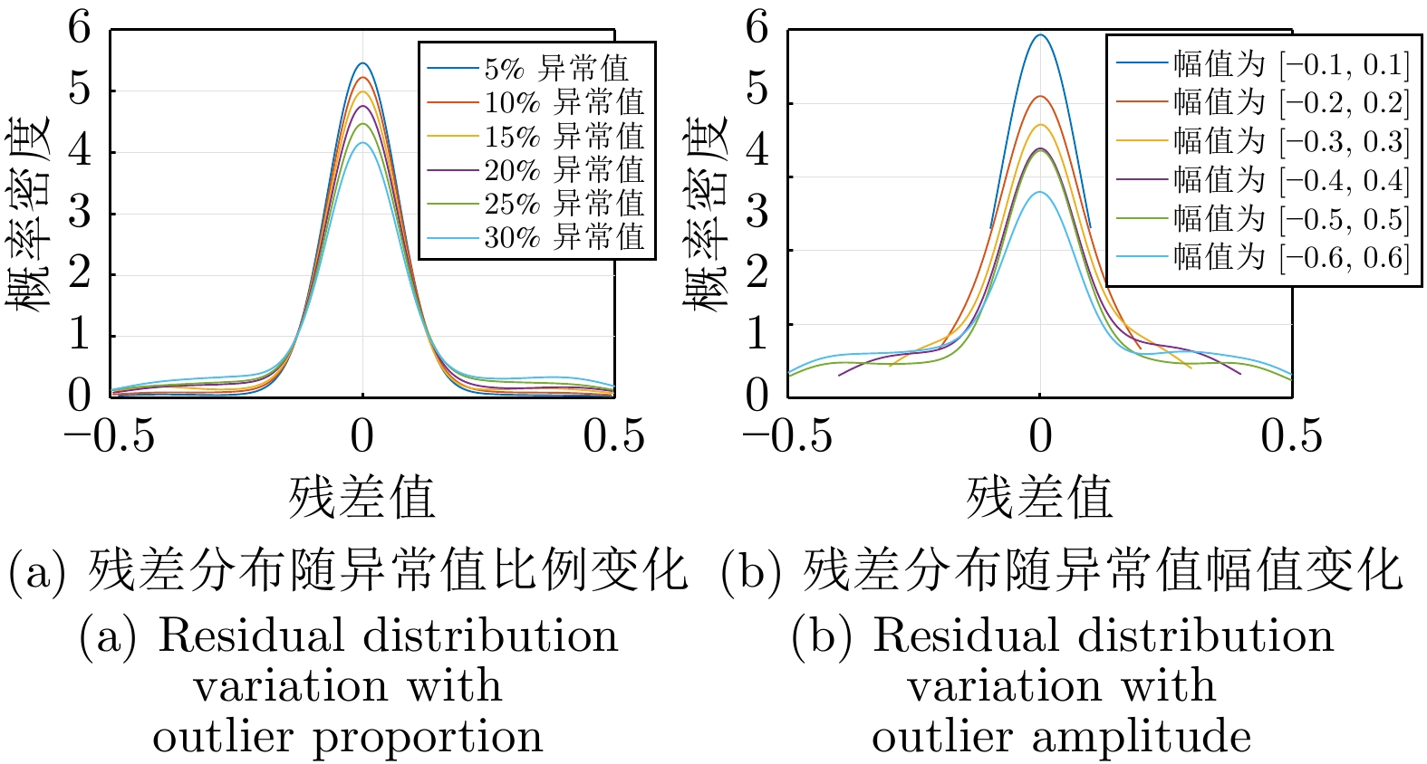
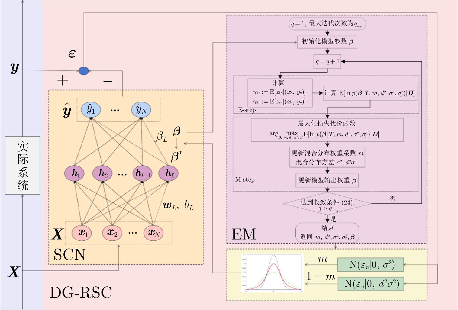
摘要: 工业过程数据常常受到混合噪声干扰, 传统基于单一重尾分布的鲁棒建模方法在处理混合噪声问题时, 在准确性与可解释性方面均存在一定局限. 基于此, 提出一种混合双高斯分布的可解释鲁棒自适应建模方法. 该方法首先采用随机配置算法构建基础的随机配置网络学习模型, 确定模型的隐含层节点数、输入权重和偏置; 其次为保证模型对混合噪声的鲁棒性, 构建双高斯分布(一大一小方差)加权组合而成的噪声表征模型; 随后利用期望最大化算法自适应迭代学习随机配置网络输出权值和混合高斯模型噪声参数, 最终形成基于双高斯分布混合鲁棒建模方法. 该方法具有以下优势: 噪声模型能够通过参数自适应学习逼近实际混合噪声特性, 其中大方差高斯分量负责对异常噪声进行粗调, 小方差高斯分量则用于精细拟合主体噪声, 从而增强模型的可解释性; 在网络模型输出权值估计过程中, 通过为每个输出数据点自适应分配惩罚权重, 保障模型的鲁棒性能. 为验证所提方法的有效性, 分别在函数仿真、基准数据集和工业实例上设计多组对比实验, 结果均表明所提方法具备良好的可靠性与实用性.Abstract: Industrial process data are often contaminated by mixed noise interference. Traditional robust modeling methods based on single heavy-tailed distributions exhibit certain limitations in both accuracy and interpretability when dealing with mixed noise problems. To address these issues, an interpretable robust adaptive modeling method based on a mixed dual Gaussian distribution is proposed. First, the proposed method begins by constructing a base learning model by using the stochastic configuration network (SCN) framework to determine the number of hidden nodes, input weights, and biases. Secondly, to ensure robustness against mixed noise, a noise characterization model is established through a weighted combination of dual Gaussian distribution with large and small variances. And then the expectation-maximization algorithm is employed to adaptively and iteratively learn both the output weights of the SCN and the parameters of the Gaussian mixture model, ultimately forming the robust stochastic configuration network model based on dual Gaussian distribution. The proposed method offers two main advantages: The noise model can approximate the characteristics of actual mixed noise through adaptive parameter learning, where the large-variance Gaussian component handles coarse approximation of anomalous noise while the small-variance Gaussian component achieves fine-grained characterization of dominant noise, thereby enhancing interpretability; During the estimation of network output weights, the model ensures robust performance by adaptively assigning penalty weights to each output data point. To validate the effectiveness of the proposed method, multiple comparative experiments are conducted on function approximation, benchmark datasets, and an industrial case study. The results consistently demonstrate that the proposed method achieves satisfactory reliability and practicality.
-
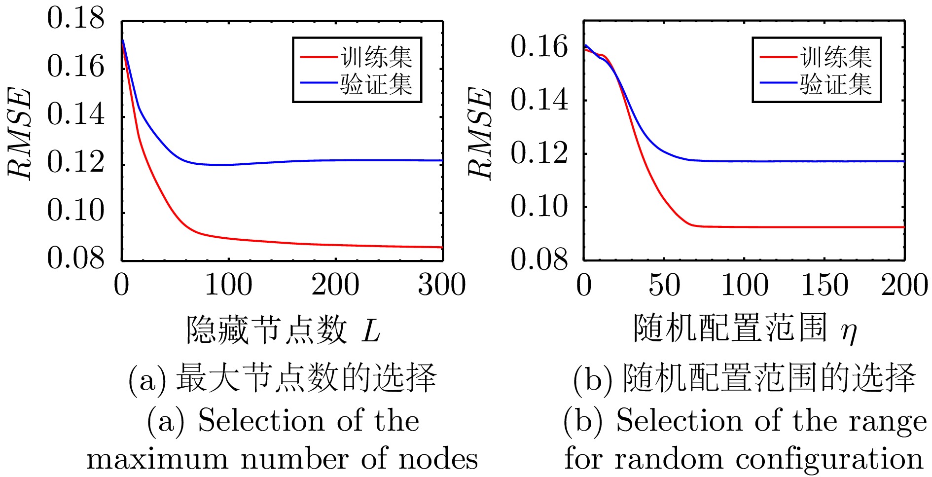
图 3 利用验证集对DG-RSC算法进行超参数选择
Fig. 3 Hyper-parameters selection of the DG-RSC algorithm by using the validation set
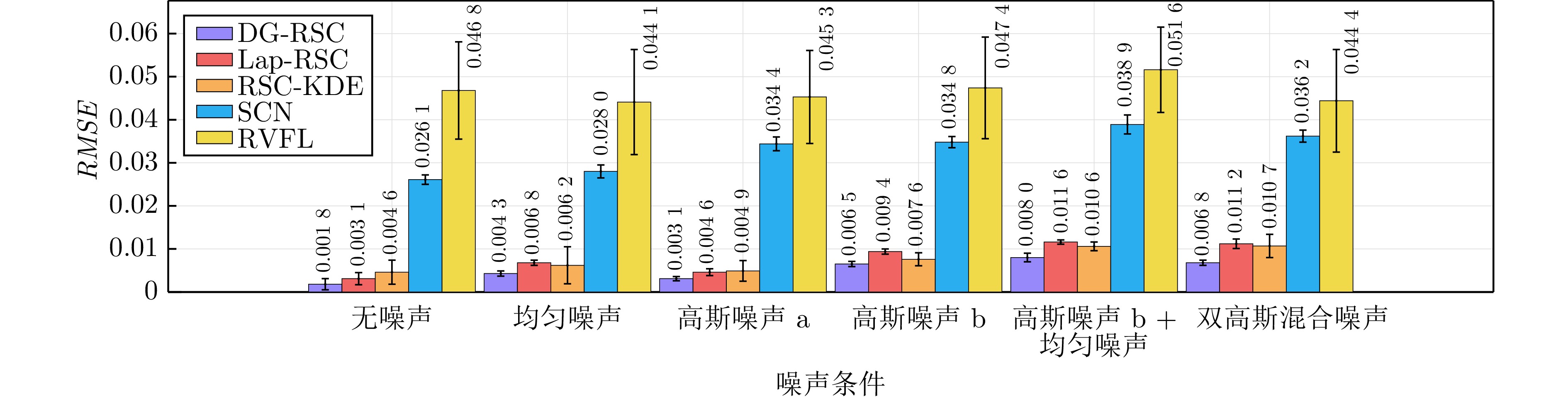
图 8 不同背景噪声条件下各算法的$ RMSE $
Fig. 8 $ RMSE $ of various algorithms under different background noise conditions
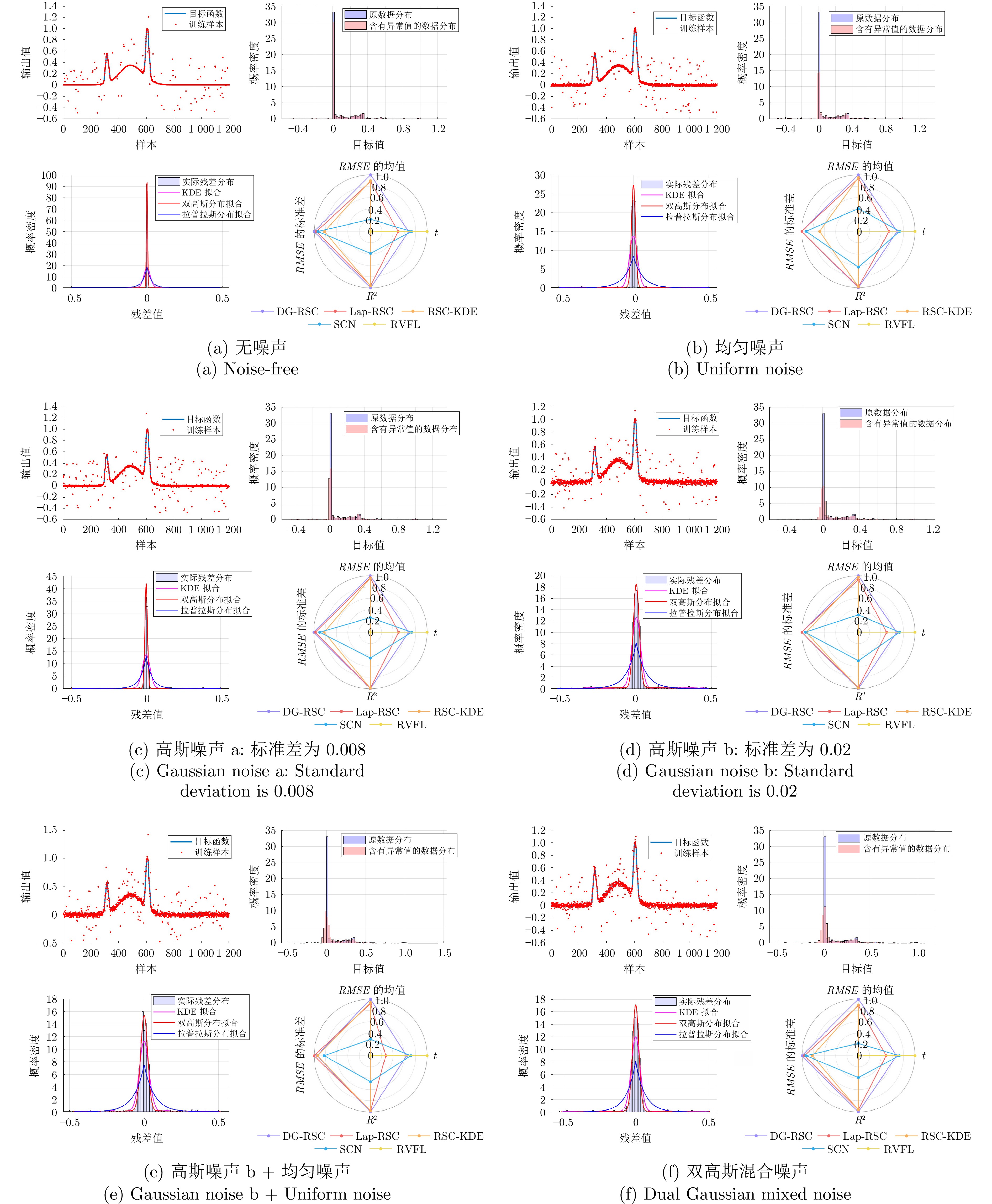
图 9 不同背景噪声条件下各算法的性能比较
Fig. 9 Performance comparison of various algorithms under different background noise conditions
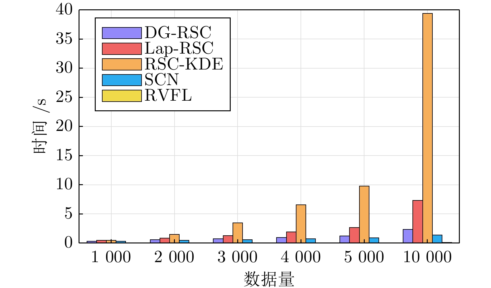
图 10 不同数据量下五种算法运行时间对比
Fig. 10 Comparison of running time of five algorithms under different data volumes
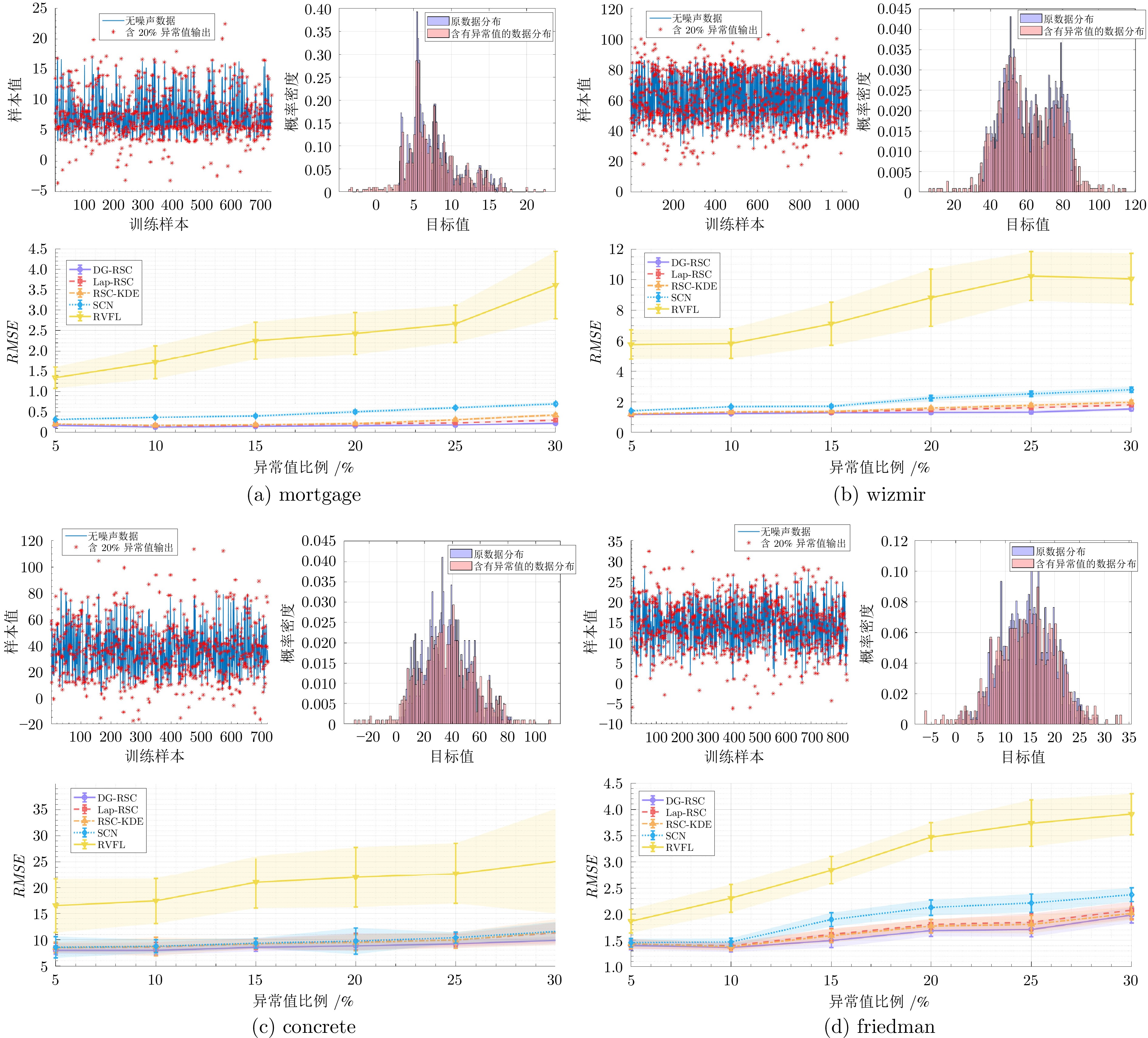
图 11 四个基准数据集上五种算法的比较结果
Fig. 11 The comparison results of five algorithms on four benchmark datasets
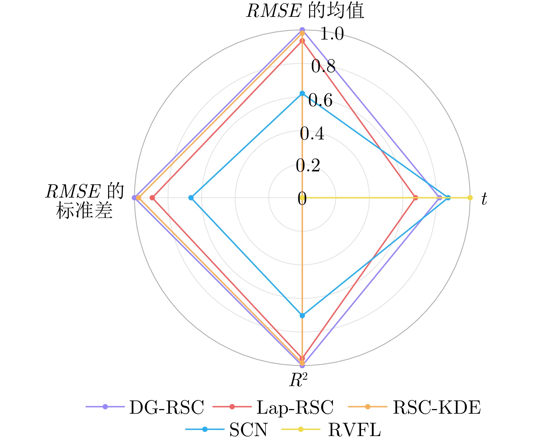
图 13 各算法在磨矿粒度预测上的雷达图
Fig. 13 Radar chart of each algorithm in the prediction of grinding particle size
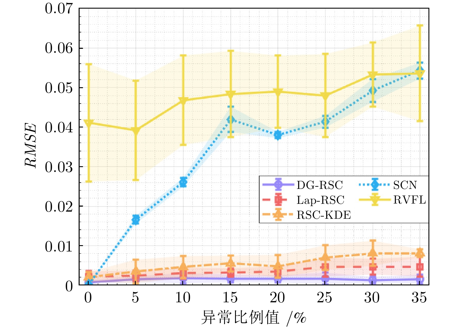
表 1 不同异常值比例下各算法的性能比较
Table 1 Performance comparison of various algorithms under different proportions of outliers
算法 异常值比例 0% 5% 10% 15% $ RMSE $ $ R^2 $ $ t ({\mathrm{s}}) $ $ RMSE $ $ R^2 $ $ t ({\mathrm{s}})$ $ RMSE $ $ R^2 $ $ t ({\mathrm{s}}) $ $ RMSE $ $ R^2 $ $ t ({\mathrm{s}}) $ DG-RSC $ 0.000\,7 \pm 0.000\,6 $ $ {{1.000\,0}} $ $ 0.390\,8 $ $ {{0.001\,5 \pm 0.000\,8}} $ $ {{0.999\,9}} $ $ 0.444\,9 $ $ {{0.001\,8 \pm 0.001\,3}} $ $ {{0.999\,8}} $ $ 0.473\,4 $ $ {{0.001\,7 \pm 0.001\,0}} $ $ {{0.999\,8}} $ $ 0.443\,5 $ Lap-RSC $ 0.002\,2 \pm 0.001\,4 $ $ 0.999\,7 $ $ 0.427\,0 $ $ 0.002\,4 \pm 0.001\,3 $ $ 0.999\,7 $ $ 0.480\,4 $ $ 0.003\,1 \pm 0.001\,4 $ $ 0.999\,5 $ $ 0.499\,3 $ $ 0.003\,2 \pm 0.001\,1 $ $ 0.999\,5 $ $ 0.535\,3 $ RSC-KDE $ 0.002\,0 \pm 0.001\,3 $ $ 0.999\,8 $ $ 1.413\,4 $ $ 0.003\,5 \pm 0.003\,0 $ $ 0.999\,1 $ $ 1.420\,7 $ $ 0.004\,6 \pm 0.002\,8 $ $ 0.998\,8 $ $ 1.434\,3 $ $ 0.005\,5 \pm 0.002\,0 $ $ 0.998\,6 $ $ 1.423\,2 $ SCN $ {{0.000\,2 \pm 0.000\,2}} $ $ {{1.000\,0}} $ $ 0.375\,2 $ $ 0.016\,6 \pm 0.001\,0 $ $ 0.988\,7 $ $ 0.381\,3 $ $ 0.026\,1 \pm 0.001\,1 $ $ 0.972\,0 $ $ 0.381\,3 $ $ 0.042\,0 \pm 0.003\,2 $ $ 0.927\,1 $ $ 0.382\,7 $ RVFL $ 0.041\,1 \pm 0.014\,9 $ $ 0.921\,7 $ $ {{0.006\,0}} $ $ 0.039\,2 \pm 0.012\,6 $ $ 0.930\,5 $ $ {{0.005\,9}} $ $ 0.046\,8 \pm 0.011\,3 $ $ 0.904\,8 $ $ {{0.005\,1}} $ $ 0.048\,4 \pm 0.010\,9 $ $ 0.898\,8 $ $ {{0.005\,9}} $ 算法 异常值比例 20% 25% 30% 35% $ RMSE $ $ R^2 $ $ t (s)$ $ RMSE $ $ R^2 $ $ t (s)$ $ RMSE $ $ R^2 $ $ t (s)$ $ RMSE $ $ R^2 $ $ t (s)$ DG-RSC $ {{0.001\,6 \pm 0.000\,9}} $ $ {{0.999\,9}} $ $ 0.446\,0 $ $ {{0.001\,7 \pm 0.001\,5}} $ $ {{0.999\,8}} $ $ 0.468\,2 $ $ {{0.001\,3 \pm 0.000\,8}} $ $ {{0.999\,9}} $ $ 0.475\,0 $ $ {{0.001\,5 \pm 0.001\,2}} $ $ {{0.999\,9}} $ $ 0.562\,4 $ Lap-RSC $ 0.003\,5 \pm 0.001\,3 $ $ 0.999\,4 $ $ 0.546\,0 $ $ 0.004\,6 \pm 0.002\,4 $ $ 0.998\,9 $ $ 0.642\,7 $ $ 0.004\,7 \pm 0.002\,0 $ $ 0.998\,9 $ $ 0.643\,1 $ $ 0.004\,7 \pm 0.002\,5 $ $ 0.998\,8 $ $ 1.280\,7 $ RSC-KDE $ 0.004\,8 \pm 0.002\,9 $ $ 0.998\,7 $ $ 1.427\,2 $ $ 0.007\,0 \pm 0.003\,1 $ $ 0.997\,6 $ $ 1.426\,9 $ $ 0.008\,1 \pm 0.003\,2 $ $ 0.996\,9 $ $ 1.421\,2 $ $ 0.008\,1 \pm 0.001\,0 $ $ 0.997\,3 $ $ 1.532\,4 $ SCN $ 0.038\,0 \pm 0.000\,8 $ $ 0.940\,8 $ $ 0.381\,1 $ $ 0.041\,4 \pm 0.001\,5 $ $ 0.929\,5 $ $ 0.377\,3 $ $ 0.049\,3 \pm 0.002\,9 $ $ 0.899\,7 $ $ 0.375\,5 $ $ 0.054\,3 \pm 0.002\,0 $ $ 0.878\,6 $ $ 0.441\,2 $ RVFL $ 0.049\,0 \pm 0.009\,1 $ $ 0.897\,9 $ $ {{0.005\,9}} $ $ 0.048\,0 \pm 0.010\,5 $ $ 0.900\,9 $ $ {{0.006\,0}} $ $ 0.053\,3 \pm 0.008\,1 $ $ 0.880\,8 $ $ {{0.006\,0}} $ $ 0.053\,6 \pm 0.012\,1 $ $ 0.876\,2 $ $ {{0.005\,9}} $  下载: 导出CSV
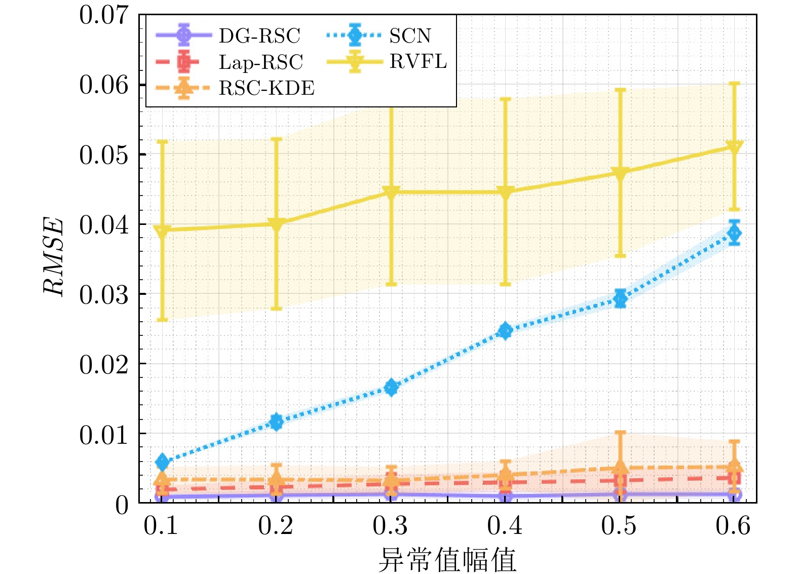
表 2 不同异常值幅值下各算法的性能比较
Table 2 Performance comparison of various algorithms under different amplitudes of outliers
算法 异常值幅值区间 $ [-0.1,\; 0.1] $ $ [-0.2,\; 0.2] $ $ [-0.3,\; 0.3] $ $ RMSE $ $ R^2 $ $ t ({\mathrm{s}}) $ $ RMSE $ $ R^2 $ $ t ({\mathrm{s}}) $ $ RMSE $ $ R^2 $ $ t ({\mathrm{s}}) $ DG-RSC $ {{0.000\,9\pm0.000\,5}} $ $ {{1.000\,0}} $ $ 0.477\,5 $ $ {{0.001\,1\pm0.000\,7}} $ $ {{0.999\,9}} $ $ 0.482\,1 $ $ {{0.001\,3\pm0.000\,7}} $ $ {{0.999\,9}} $ $ 0.493\,0 $ Lap-RSC $ 0.001\,9\pm0.000\,6 $ $ 0.999\,8 $ $ 0.473\,2 $ $ 0.002\,3\pm0.001\,0 $ $ 0.999\,7 $ $ 0.507\,2 $ $ 0.002\,7\pm0.001\,4 $ $ 0.999\,6 $ $ 0.536\,1 $ RSC-KDE $ 0.003\,3\pm0.001\,9 $ $ 0.999\,4 $ $ 1.405\,2 $ $ 0.003\,3\pm0.002\,1 $ $ 0.999\,4 $ $ 1.436\,5 $ $ 0.003\,2\pm0.002\,0 $ $ 0.999\,4 $ $ 1.464\,2 $ SCN $ 0.005\,8\pm0.000\,2 $ $ 0.998\,6 $ $ 0.394\,0 $ $ 0.011\,6\pm0.000\,7 $ $ 0.994\,5 $ $ 0.400\,6 $ $ 0.016\,5\pm0.000\,6 $ $ 0.988\,8 $ $ 0.411\,8 $ RVFL $ 0.039\,0\pm0.012\,8 $ $ 0.930\,9 $ $ {{0.006\,1}} $ $ 0.040\,0\pm0.012\,2 $ $ 0.928\,1 $ $ {{0.005\,9}} $ $ 0.044\,6\pm0.013\,3 $ $ 0.911\,1 $ $ {{0.006\,2}} $ 算法 异常值幅值区间 $ [-0.4,\; 0.4] $ $ [-0.5,\; 0.5] $ $ [-0.6,\; 0.6] $ $ RMSE $ $ R^2 $ $ t ({\mathrm{s}}) $ $ RMSE $ $ R^2 $ $ t ({\mathrm{s}}) $ $ RMSE $ $ R^2 $ $ t ({\mathrm{s}}) $ DG-RSC $ {{0.001\,0\pm0.000\,7}} $ $ {{0.999\,9}} $ $ 0.483\,8 $ $ {{0.001\,2\pm0.000\,7}} $ $ {{0.999\,9}} $ $ 0.479\,2 $ $ {{0.001\,2\pm0.000\,7}} $ $ {{0.999\,9}} $ $ 0.480\,7 $ Lap-RSC $ 0.003\,0\pm0.001\,3 $ $ 0.999\,6 $ $ 0.516\,9 $ $ 0.003\,2\pm0.001\,7 $ $ 0.999\,5 $ $ 0.592\,4 $ $ 0.003\,6\pm0.001\,9 $ $ 0.999\,3 $ $ 0.594\,1 $ RSC-KDE $ 0.004\,0\pm0.002\,9 $ $ 0.999\,0 $ $ 1.420\,4 $ $ 0.005\,0\pm0.005\,1 $ $ 0.997\,9 $ $ 1.423\,3 $ $ 0.005\,2\pm0.003\,6 $ $ 0.998\,4 $ $ 1.422\,7 $ SCN $ 0.024\,6\pm0.001\,2 $ $ 0.975\,1 $ $ 0.382\,2 $ $ 0.029\,3\pm0.001\,1 $ $ 0.964\,6 $ $ 0.395\,4 $ $ 0.038\,7\pm0.001\,6 $ $ 0.938\,5 $ $ 0.383\,5 $ RVFL $ 0.044\,6\pm0.012\,7 $ $ 0.911\,8 $ $ {{0.005\,5}} $ $ 0.047\,3\pm0.011\,9 $ $ 0.902\,3 $ $ {{0.006\,0}} $ $ 0.051\,1\pm0.009\,0 $ $ 0.889\,5 $ $ {{0.006\,0}} $
下载: 导出CSV
表 3 不同背景噪声条件下各算法的性能比较
Table 3 Performance comparison of various algorithms under different background noise conditions
算法 噪声条件 无噪声 均匀噪声$ {\rm{U}}(-0.02,\; 0.02) $ 高斯噪声a: 标准差为0.008 $ RMSE $ $ R^2 $ $ t ({\mathrm{s}}) $ $ RMSE $ $ R^2 $ $ t ({\mathrm{s}}) $ $ RMSE $ $ R^2 $ $ t ({\mathrm{s}}) $ DG-RSC $ {{0.001\,8 \pm 0.001\,3}} $ $ {{0.999\,8}} $ $ 0.473\,4 $ $ {{0.004\,3 \pm 0.000\,6}} $ $ {{0.999\,2}} $ $ 0.466\,3 $ $ {{0.003\,1 \pm 0.000\,5}} $ $ {{0.999\,6}} $ $ 0.478\,8 $ Lap-RSC $ 0.003\,1 \pm 0.001\,4 $ $ 0.999\,5 $ $ 0.499\,3 $ $ 0.006\,8 \pm 0.000\,6 $ $ 0.998\,1 $ $ 0.678\,8 $ $ 0.004\,6 \pm 0.000\,8 $ $ 0.999\,1 $ $ 0.735\,9 $ RSC-KDE $ 0.004\,6 \pm 0.002\,8 $ $ 0.998\,8 $ $ 1.434\,3 $ $ 0.006\,2 \pm 0.004\,3 $ $ 0.997\,7 $ $ 1.472\,9 $ $ 0.004\,9 \pm 0.002\,4 $ $ 0.998\,8 $ $ 1.462\,1 $ SCN $ 0.026\,1 \pm 0.001\,1 $ $ 0.972\,0 $ $ 0.381\,3 $ $ 0.028\,0 \pm 0.001\,5 $ $ 0.967\,7 $ $ 0.400\,1 $ $ 0.034\,4 \pm 0.001\,6 $ $ 0.951\,2 $ $ 0.399\,3 $ RVFL $ 0.046\,8 \pm 0.011\,3 $ $ 0.904\,8 $ $ {{0.005\,1}} $ $ 0.044\,1 \pm 0.012\,2 $ $ 0.914\,1 $ $ {{0.005\,6}} $ $ 0.045\,3 \pm 0.010\,8 $ $ 0.910\,8 $ $ {{0.005\,4}} $ 算法 噪声条件 高斯噪声b: 标准差为0.02 高斯噪声b + 均匀噪声 双高斯混合噪声: 高斯噪声a + 高斯噪声b $ RMSE $ $ R^2 $ $ t ({\mathrm{s}}) $ $ RMSE $ $ R^2 $ $ t ({\mathrm{s}}) $ $ RMSE $ $ R^2 $ $ t ({\mathrm{s}}) $ DG-RSC $ {{0.006\,5 \pm 0.000\,6 }} $ $ {{0.998\,3}} $ $ 0.475\,5 $ $ {{0.008\,0 \pm 0.001\,0}} $ $ {{0.997\,3}} $ $ 0.569\,1 $ $ {{0.006\,8 \pm 0.000\,6}} $ $ {{0.998\,1}} $ $ 0.480\,1 $ Lap-RSC $ 0.009\,4 \pm 0.000\,6 $ $ 0.996\,4 $ $ 0.732\,9 $ $ 0.011\,6 \pm 0.000\,5 $ $ 0.994\,4 $ $ 1.142\,4 $ $ 0.011\,2 \pm 0.001\,1 $ $ 0.994\,8 $ $ 0.755\,0 $ RSC-KDE $ 0.007\,6 \pm 0.001\,5 $ $ 0.997\,5 $ $ 1.467\,7 $ $ 0.010\,6 \pm 0.001\,1 $ $ 0.995\,3 $ $ 1.567\,7 $ $ 0.010\,7 \pm 0.002\,7 $ $ 0.995\,0 $ $ 1.472\,2 $ SCN $ 0.034\,8 \pm 0.001\,3 $ $ 0.950\,2 $ $ 0.399\,8 $ $ 0.038\,9 \pm 0.002\,2 $ $ 0.937\,7 $ $ 0.449\,2 $ $ 0.036\,2 \pm 0.001\,4 $ $ 0.946\,1 $ $ 0.409\,2 $ RVFL $ 0.047\,4 \pm 0.011\,8 $ $ 0.902\,0 $ $ {{0.005\,5}} $ $ 0.051\,6 \pm 0.009\,9 $ $ 0.886\,6 $ $ {{0.005\,9}} $ $ 0.044\,4 \pm 0.011\,9 $ $ 0.913\,2 $ $ {{0.005\,5}} $
下载: 导出CSV
表 4 不同数据量下五种算法运行时间对比(s)
Table 4 Comparison of running time of five algorithms under different data volumes (s)
算法 数据量 1000 2000 3000 4000 5000 10000 DG-RSC 0.3342 0.5570 0.7510 0.9320 1.2130 2.3480 Lap-RSC 0.4510 0.8640 1.2940 1.9290 2.6610 7.3280 RSC-KDE 0.4930 1.5040 3.4770 6.5760 9.7990 39.4130 SCN 0.3140 0.4940 0.5960 0.7590 0.9160 1.3980 RVFL 0.0120 0.0270 0.0300 0.0350 0.0450 0.0690
下载: 导出CSV
表 5 不同数据集上各算法在不同异常值比例下的性能比较
Table 5 Performance comparison of various algorithms on different datasets under different proportions of outliers
数据集 算法 异常值比例 5% 10% 15% 20% 25% 30% mortgage DG-RSC $ {{0.169\,3 \pm 0.014\,6}} $ $ {{0.128\,8 \pm 0.007\,7}} $ $ {{0.147\,5 \pm 0.010\,7}} $ $ {{0.161\,0 \pm 0.013\,7}} $ $ {{0.178\,0 \pm 0.014\,3}} $ $ {{0.220\,3 \pm 0.016\,0}} $ Lap-RSC $ 0.209\,6 \pm 0.018\,0 $ $ 0.165\,1 \pm 0.010\,9 $ $ 0.174\,8 \pm 0.011\,6 $ $ 0.206\,7 \pm 0.021\,8 $ $ 0.235\,9 \pm 0.018\,3 $ $ 0.302\,6 \pm 0.032\,4 $ RSC-KDE $ 0.202\,8 \pm 0.016\,7 $ $ 0.173\,4 \pm 0.012\,2 $ $ 0.193\,7 \pm 0.013\,9 $ $ 0.218\,8 \pm 0.027\,0 $ $ 0.309\,7 \pm 0.030\,8 $ $ 0.422\,4 \pm 0.040\,7 $ SCN $ 0.316\,0 \pm 0.021\,2 $ $ 0.366\,5 \pm 0.020\,9 $ $ 0.404\,3 \pm 0.028\,5 $ $ 0.504\,4 \pm 0.038\,8 $ $ 0.605\,3 \pm 0.032\,3 $ $ 0.699\,2 \pm 0.039\,0 $ RVFL $ 1.339\,0 \pm 0.260\,2 $ $ 1.716\,9 \pm 0.405\,0 $ $ 2.248\,1 \pm 0.455\,6 $ $ 2.424\,9 \pm 0.513\,5 $ $ 2.663\,2 \pm 0.452\,5 $ $ 3.611\,4 \pm 0.822\,3 $ wizmir DG-RSC $ {{1.159\,9 \pm 0.027\,8}} $ $ {{1.219\,1 \pm 0.048\,0}} $ $ {{1.276\,8 \pm 0.074\,4}} $ $ {{1.292\,9 \pm 0.111\,2}} $ $ {{1.327\,3 \pm 0.119\,8}} $ $ {{1.521\,9 \pm 0.115\,4}} $ Lap-RSC $ 1.185\,4 \pm 0.030\,1 $ $ 1.312\,0 \pm 0.056\,9 $ $ 1.326\,4 \pm 0.055\,4 $ $ 1.466\,8 \pm 0.093\,8 $ $ 1.608\,6 \pm 0.096\,6 $ $ 1.796\,0 \pm 0.110\,3 $ RSC-KDE $ 1.195\,6 \pm 0.041\,2 $ $ 1.334\,1 \pm 0.041\,4 $ $ 1.362\,2 \pm 0.062\,6 $ $ 1.580\,6 \pm 0.104\,8 $ $ 1.773\,8 \pm 0.109\,3 $ $ 1.979\,6 \pm 0.116\,2 $ SCN $ 1.413\,8 \pm 0.066\,9 $ $ 1.671\,7 \pm 0.075\,7 $ $ 1.702\,0 \pm 0.099\,4 $ $ 2.230\,5 \pm 0.179\,5 $ $ 2.504\,2 \pm 0.181\,6 $ $ 2.776\,5 \pm 0.187\,3 $ RVFL $ 5.754\,1 \pm 0.970\,6 $ $ 5.814\,0 \pm 0.980\,5 $ $ 7.111\,0 \pm 1.412\,0 $ $ 8.817\,9 \pm 1.861\,9 $ $ 10.223\,5 \pm 1.600\,2\ \,$ $ 10.045\,8 \pm 1.667\,8\ \, $ concrete DG-RSC $ {{7.918\,5 \pm 0.700\,9}} $ $ {{7.966\,0 \pm 0.863\,4}} $ $ {{8.568\,4 \pm 0.818\,1}} $ $ {{8.809\,3 \pm 0.786\,8}} $ $ {{9.167\,3 \pm 0.715\,4}} $ $ {{9.839\,6 \pm 0.748\,0}} $ Lap-RSC $ 8.444\,0 \pm 0.900\,9 $ $ 8.593\,9 \pm 0.898\,5 $ $ 9.194\,6 \pm 1.077\,4 $ $ 9.572\,4 \pm 1.629\,3 $ $ 9.923\,7 \pm 1.192\,8 $ $ 11.273\,6 \pm 1.961\,7\ \, $ RSC-KDE $ 8.506\,0 \pm 1.037\,0 $ $ 8.674\,1 \pm 1.753\,4 $ $ 9.200\,1 \pm 0.933\,6 $ $ 9.432\,3 \pm 1.551\,0 $ $ 9.888\,4 \pm 1.525\,8 $ $ 11.429\,9 \pm 2.474\,0 \ \,$ SCN $ 8.553\,8 \pm 2.045\,0 $ $ 8.749\,3 \pm 1.263\,2 $ $ 9.320\,6 \pm 0.993\,6 $ $ 9.740\,9 \pm 2.502\,6 $ $ 10.361\,5 \pm 1.043\,8\ \,$ $ 11.535\,6 \pm 1.882\,9 \ \,$ RVFL $ 16.506\,5 \pm 5.148\,0\ \, $ $ 17.422\,4 \pm 4.351\,1 \ \,$ $ 21.045\,2 \pm 5.233\,7\ \, $ $ 21.988\,3 \pm 5.789\,8 \ \,$ $ 22.751\,9 \pm 5.831\,4\ \,$ $ 25.075\,4 \pm 10.085\,9 $ friedman DG-RSC $ {{1.406\,5 \pm 0.086\,8}} $ $ {{1.362\,8 \pm 0.082\,0}} $ $ {{1.496\,5 \pm 0.132\,3}} $ $ {{1.685\,6 \pm 0.108\,7}} $ $ {{1.708\,8 \pm 0.138\,3}} $ $ {{1.980\,8 \pm 0.149\,6}} $ Lap-RSC $ 1.430\,9 \pm 0.089\,6 $ $ 1.397\,0 \pm 0.072\,8 $ $ 1.611\,3 \pm 0.112\,3 $ $ 1.805\,4 \pm 0.094\,2 $ $ 1.845\,6 \pm 0.160\,9 $ $ 2.072\,9 \pm 0.162\,1 $ RSC-KDE $ 1.435\,3 \pm 0.093\,7 $ $ 1.380\,1 \pm 0.073\,5 $ $ 1.586\,4 \pm 0.127\,5 $ $ 1.774\,0 \pm 0.130\,8 $ $ 1.805\,6 \pm 0.171\,3 $ $ 2.017\,6 \pm 0.127\,0 $ SCN $ 1.453\,5 \pm 0.080\,4 $ $ 1.466\,3 \pm 0.074\,3 $ $ 1.894\,0 \pm 0.132\,1 $ $ 2.122\,9 \pm 0.149\,1 $ $ 2.208\,4 \pm 0.174\,8 $ $ 2.371\,5 \pm 0.133\,2 $ RVFL $ 1.865\,6 \pm 0.222\,2 $ $ 2.301\,1 \pm 0.270\,0 $ $ 2.843\,8 \pm 0.259\,9 $ $ 3.474\,7 \pm 0.274\,2 $ $ 3.737\,6 \pm 0.445\,3 $ $ 3.909\,9 \pm 0.389\,4 $
下载: 导出CSV
表 6 各算法在磨矿粒度预测上的性能表现
Table 6 The performance of each algorithm in the prediction of grinding particle size
算法 $ RMSE $ $ R^2 $ $ t ({\mathrm{s}})$ DG-RSC $ {{0.245\,7\pm0.000\,7}} $ $ {{0.991\,2}} $ $ 0.089\,6 $ Lap-RSC $ 0.262\,3\pm0.003\,7 $ $ 0.990\,0 $ $ 0.154\,6 $ RSC-KDE $ 0.250\,8 \pm 0.001\,4 $ $ 0.990\,8 $ $ 0.461\,4 $ SCN $ 0.342\,3 \pm 0.010\,2 $ $ 0.982\,9 $ $ 0.066\,4 $ RVFL $ 0.500\,9 \pm 0.028\,6 $ $ 0.963\,3 $ $ {{0.006\,9}} $
下载: 导出CSV
-
[1] Peter O, Anup P, Nelson S M, Samuel A A, Christian O O, Diarah R S. Integration of AI and IoT in smart manufacturing: Exploring technological, ethical, and legal frontiers. Procedia Computer Science, 2025, 253: 654−660 doi: 10.1016/j.procs.2025.01.127 [2] Zhao C, Zhao T N, Sun H, Yang H N. Study on droplet freezing process based on the combination of multiwavelength absorption spectroscopy and data-driven model. Measurement, 2025, 255: Article No. 118083 doi: 10.1016/j.measurement.2025.118083 [3] Agostino M, Alessandro P, Vito S. An efficient cardiovascular disease prediction model through AI-driven IoT technology. Computers in Biology and Medicine, 2024, 183: Article No. 109330 [4] 代伟, 张政煊, 杨春雨, 马小平. 基于SCN数据模型的SISO非线性自适应控制. 自动化学报, 2024, 50(10): 2002−2012 doi: 10.16383/j.aas.c210174Dai Wei, Zhang Zheng-Xuan, Yang Chun-Yu, Ma Xiao-Ping. Adaptive control of SISO nonlinear system using data-driven SCN model. Acta Automatica Sinica, 2024, 50(10): 2002−2012 doi: 10.16383/j.aas.c210174 [5] Lee S, Sohn I. Accurate prediction of high-temperature ionic melt viscosity through data-driven modeling enhanced with explainable AI. Journal of Materials Science and Technology, 2025, 248: 110−118 [6] Xie C R, Chen X. A robust data-driven approach for modeling industrial systems with non-stationary and sparsely sampled data streams. Journal of Process Control, 2025, 150: Article No. 103425 doi: 10.1016/j.jprocont.2025.103425 [7] Xu L B, Zhang G, Huang X X, He L. Adaptive stochastic resonance in an improved Izhikevich neuron model driven by multiplicative and additive Gaussian noise and its application in fault diagnosis of wind turbines. Renewable Energy, 2025, 253: Article No. 123566 [8] Cheng Y K, Zhan H F, Yu J H, Wang R. Data-driven online prediction and control method for injection molding product quality. Journal of Manufacturing Processes, 2025, 145: 252−273 doi: 10.1016/j.jmapro.2025.04.054 [9] Zhang L M Q, Zhu L P, Wen W J, Li J Y, Zhang C. Three-stage composite outlier identification of wind power data: Integrating physical rules with regression learning and mathematical morphology. IEEE Transactions on Instrumentation and Measurement, 2025, 74: Article No. 9004613 [10] Zhang C, Li Z B, Ge Y D, Liu Q L, Suo L M, Song S H, et al. Enhancing short-term wind speed prediction based on an outlier-robust ensemble deep random vector functional link network with AOA-optimized VMD. Energy, 2024, 296: Article No. 131173 doi: 10.1016/j.energy.2024.131173 [11] Jia W N, Li X F, Bi D J, Xie Y L. Maximum mixture correntropy based student-t kernel adaptive filtering for indoor positioning of internet of things. Information Sciences, 2025, 696: Article No. 121729 doi: 10.1016/j.ins.2024.121729 [12] Liu W T, Li S Y. Monitoring large-scale industrial systems for wastewater treatment processes with process noise using data-driven NARX approach. Control Engineering Practice, 2025, 16: Article No. 106321 doi: 10.1016/j.conengprac.2025.106321 [13] Wang X Y, Yan X Z, Luo Q H. Adaptive square-root extended cubature Kalman filter based on Huber M-estimation for multi-AUV cooperative navigation. Measurement, 2025, 249: Article No. 117035 [14] Luo B, Gao X L. High-dimensional robust approximated M-estimators for mean regression with asymmetric data. arXiv preprint arXiv: 1910.09493, 2022. [15] Cao B H, Yin Q S, Guo Y Y, Yang J, Zhang L B, Wang Z Q, et al. Field data analysis and risk assessment of shallow gas hazards based on neural networks during industrial deep-water drilling. Reliability Engineering & System Safety, 2023, 232: Article No. 109079 doi: 10.1016/j.ress.2022.109079 [16] Yu Z H, Zhang Z Y, Jiang Q C, Yan X F. Neural network-based hybrid modeling approach incorporating Bayesian optimization with industrial soft sensor application. Knowledge-Based Systems, 2024, 301: Article No. 112341 doi: 10.1016/j.knosys.2024.112341 [17] Fang X H, Song Q H, Wang X J, Li Z Y, Ma H F, Liu Z Q. An intelligent tool wear monitoring model based on knowledge-data-driven physical-informed neural network for digital twin milling. Mechanical Systems and Signal Processing, 2025, 232: Article No. 112736 doi: 10.1016/j.ymssp.2025.112736 [18] Yu F, Su D, He S Q, Wu Y Y, Zhang S K, Yin H G. Resonant tunneling diode cellular neural network with memristor coupling and its application in police forensic digital image protection. Chinese Physics B, 2025, 34(5): 287−300 doi: 10.1088/1674-1056/adb8bb [19] 谭帅, 王一帆, 姜庆超, 侍洪波, 宋冰. 基于不同故障传播路径差异化的故障诊断方法. 自动化学报, 2025, 51(1): 161−173 doi: 10.16383/j.aas.c240151Tan Shuai, Wang Yi-Fan, Jiang Qing-Chao, Shi Hong-Bo, Song Bing. Fault propagation path-aware network: A fault diagnosis method. Acta Automatica Sinica, 2025, 51(1): 161−173 doi: 10.16383/j.aas.c240151 [20] Pao Y H, Takefuji Y. Functional-link net computing: Theory, system architecture, and functionalities. Computer, 1992, 25(5): 76−79 doi: 10.1109/2.144401 [21] Wang D H, Li M. Stochastic configuration networks: Fundamentals and algorithms. IEEE Transactions on Cybernetics, 2017, 47(10): 3346−3479 doi: 10.1109/tcyb.2017.2734043 [22] Sun K, Yang C P, Gao C, Wu X L, Zhao J J. Development of an online updating stochastic configuration network for the soft-sensing of the semi-autogenous ball mill crusher system. IEEE Transactions on Instrumentation and Measurement, 2024, 73: Article No. 2506111 doi: 10.1109/tim.2023.3348909 [23] Yan A J, Hu K C, Wang D H. Monitoring model based on data-driven optimization stochastic configuration network and its applications. IEEE Sensors Journal, 2025, 25(6): 10087−10096 doi: 10.1109/JSEN.2025.3538942 [24] Guo Y N, Pu J Y, He J L, Jiao B T, Ji J J, Yang S X. Adaptive stochastic configuration network based on online active learning for evolving data streams. Information Sciences, 2025, 711: Article No. 122113 [25] Zhu J Z, Zhang L, Zhang D, Chen Y X. Probabilistic wind power prediction using incremental Bayesian stochastic configuration network under concept drift environment. IEEE Transactions on Industry Applications, 2025, 61(1): 1399−1409 doi: 10.1109/TIA.2024.3462696 [26] Wang D H, Tian P X, Dai W, Yu G. Predicting particle size of copper ore grinding with stochastic configuration networks. IEEE Transactions on Industrial Informatics, 2024, 20(11): 12969−12978 doi: 10.1109/TII.2024.3431039 [27] Wang D H, Li M. Robust stochastic configuration networks with kernel density estimation for uncertain data regression. Information Sciences, 2017, 412−413: 210−222 doi: 10.1016/j.ins.2017.05.047 [28] Yan A J, Guo J C, Wang D H. Robust stochastic configuration networks for industrial data modelling with student' s-t mixture distribution. Information Sciences, 2022, 606: 493−505 doi: 10.1016/j.ins.2022.05.105 [29] Lu J, Ding J. Mixed-distribution-based robust stochastic configuration networks for prediction interval construction. IEEE Transactions on Industrial Informatics, 2020, 16(8): 5099−5109 doi: 10.1109/TII.2019.2954351 [30] Liu X, Liu X Q, Dai W. Robust SCN for data-driven modeling based on heavy-tailed noise distribution. IEEE Transactions on Instrumentation and Measurement, 2025, 74: Article No. 5013713 doi: 10.1109/tim.2025.3547532 [31] 刘鑫. 时滞取值概率未知下的线性时滞系统辨识方法. 自动化学报, 2023, 49(10): 2136−2144Liu Xin. Identification of linear time-delay systems with unknown delay distributions in its value range. Acta Automatica Sinica, 2023, 49(10): 2136−2144 [32] Chen X, Zhao S, Liu F, Tao C B. Laplace distribution based online identification of linear systems with robust recursive expectation-maximization algorithm. IEEE Transactions on Industrial Informatics, 2023, 19(8): 9028−9036 doi: 10.1109/TII.2022.3225026 [33] He J C, Peng B, Wang G. A non-linear non-Gaussian filtering framework based on the Gaussian noise model jump assumption. Automatica, 2025, 178: Article No. 112360 doi: 10.1016/j.automatica.2025.112360 [34] Li Z H, Hou B, Wu Z T, Guo Z X, Ren B, Guo X P, et al. Complete rotated localization loss based on super-Gaussian distribution for remote sensing images. IEEE Transactions on Geoscience and Remote Sensing, 2023, 61(8): Article No. 5618614 doi: 10.1109/tgrs.2023.3305578 [35] Jin X, Huang B. Robust identification of piecewise/switching autoregressive exogenous process. AIChE Journal, 2010, 56(7): 1829−1844 doi: 10.1002/aic.12112 [36] Schneider F, Papaioannou I, Sudret B, Müller G. Maximum a posteriori estimation for linear structural dynamics models using Bayesian optimization with rational polynomial chaos expansions. Computer Methods in Applied Mechanics and Engineering, 2024, 432: Article No. 117418 doi: 10.1016/j.cma.2024.117418 [37] Alcalá-Fdez J, Fernandez A, Luengo J, Derrac J, García S, Sánchez L, et al. KEEL data-mining software tool: Data set repository, integration of algorithms and experimental analysis framework. Multiple-Valued Logic and Soft Computing, 2011, 17(2−3): 255−287 [38] 姚雷, 吴迪, 谢永鑫. 磨矿过程理论及设备研究进展. 选煤技术, 2023, 51(2): 1−8 doi: 10.16447/j.cnki.cpt.2023.02.001Yao Lei, Wu Di, Xie Yong-Xin. Progress of research on grinding process theory and equipment. Coal Preparation Technology, 2023, 51(2): 1−8 doi: 10.16447/j.cnki.cpt.2023.02.001 [39] Guo W, Guo K Q. Effect of solid concentration on particle size distribution and grinding kinetics in stirred mills. Minerals, 2024, 14(7): Article No. 720 doi: 10.3390/min14070720 -

 下载:
下载:

计量
- 文章访问数: 470
- HTML全文浏览量: 397
- PDF下载量: 142
- 被引次数: 0
