

Optimal Control of ATO System with Individual Components and Product Demands Based on Markov Decision Process
-
摘要: 研究多维组件, 单一产品的双需求型面向订单装配(Assemble-to-order, ATO)系统. 产品需求为延期交货型, 当其不被满足时将产生缺货等待成本; 而独立组件需求为销售损失型, 其不被满足时将产生缺货损失成本. 该问题可以抽象成一个动态马尔科夫决策过程(Markov decision process, MDP), 通过对双需求模型求解得到状态依赖型最优策略, 即任一组件的最优生产--库存策略由系统内其他组件的库存水平决定. 研究解决了多需求复杂ATO系统的生产和库存优化控制问题. 提出在一定条件下, 组件的基础库存值可以等价于最终产品需求的库存配给值. 组件的基础库存值与库存配给值随系统内其他组件库存的增加而增加, 而产品需求的库存配给值随系统组件库存和产品缺货量的增加而减少. 最后通过数值实验分析缺货量及组件库存对最优策略结构的影响, 并得到了相应的企业生产实践的管理启示.Abstract: An assemble-to-order (ATO) system is considered which produces n components to be assembled into a single product. Demand for the product is backlogged while demand for components is lost, if it is not immediately satisfied. The problem is to control component production and component inventory allocation. The Markov decision process (MDP) framework is used to formulate this problem. It is shown that for components, the optimal policy is characterized by two state-dependent thresholds: a production base-stock level and an inventory rationing level, and that for the assembled product, the optimal policy is characterized by a state-dependent rationing level. Under a certain condition, the base-stock level of component equals the rationing level for the product. The base-stock level and rationing level of one component are both increasing with the inventories of other components. The rationing level of the product is decreasing with the backlog level and other components' inventories. Finally, though some numerical examples, the influence of the backlog level and inventory level on the optimal policy is studied and some managerial insights for manufacturing practice are also provided.
-
随着全球市场竞争加剧,大规模定制已经成为生产制造企业的主要目标.客户对产品需求越来越多样化、个性化,激烈的市场竞争对企业快速响应能力的要求也越来越高.面向订单装配(Assemble-to-order,ATO)系统以低组件库存、短产品交货期和灵活反应等特点更好地满足客户对产品的个性化需求. ATO可以看作是一种流行的管理策略,已经被广泛地应用在生产制造业中,并成为制造型企业首选的生产方式之一. ATO系统由众多组件和产品组成,是一个由组件装配成成品或半成品,并以最终产品满足客户需求的过程.系统有限的库存量,需求的不确定性及产品需求与组件相互关联等因素,增加了ATO系统管理的难度.管理ATO的难点在于如何优化控制系统组件的库存,即确定最优的生产补给和需求分配策略. ATO系统是一种即时的需求响应系统.在ATO系统中库存仅为组件库存,当需求来临时组件可以立即装配成产品满足客户需求. Song等[1]研究具有泊松需求和常数再补给基础库存系统,指出产品需求满足率可以通过一系列批量分布和泊松分布的卷积得到.
De Véricourt等[2]研究两维产品需求且缺货候补型(Make to stock,MTS)系统,提出产品生产的最优策略为转换曲线"Switching curve". Karaarslan等[3]研究两个组件装配成一个最终产品且生产提前期不同的ATO系统,得到了平衡基础库存策略. Saidane等[4]研究需求到达时间间隔为爱尔朗分布(Erlang distribution)、需求量为伽玛分布(Gamma distribution)的一阶段式批量生产系统.采用上界和下界法对基础库存值加以逼近,得到了最优的生产控制策略. Juan等[5]提出一个模拟与启发式算法相结合的方法(Simheuristic algorithm)解决单生产周期随机库存缺货问题,利用柔性补给策略减少生产系统的预期总成本.另外,连续时间系统的动态马尔科夫决策过程(Markov decision process,MDP)也是近年来ATO系统研究热点.此研究方向的优秀著作之一为文献[6],Benjaafar等研究单一产品且多维产品需求ATO系统的组件库存优化控制问题,确立了明确的最优生产-库存策略. ElHafsi等[7]基于一个1维产品,$n$维组件装配结构的ATO系统,研究产品售后市场为销售损失型(Lost sales)的独立组件需求模型.研究结果表明,系统组件库存增加将导致产品需求率增加,因此需求配给水平值也会随之升高.我国学者对生产运作系统也有相关研究,娄山佐等[8-9]研究随机中断和退货环境下供应链系统的库存控制问题,利用水平穿越法得到系统的最优库存策略.郭佳等[10]以一个单产品ATO系统为研究对象,研究生产商的最优库存和生产决策,并得到了基于目标追踪法和工程深度指示的同步生产计划方法.刘艳梅等[11]针对大批量定制模式下的ATO产品的提前期设置,零部件加工与产品装配同步的问题,提出最优的产品装配计划方法.
以上研究只针对产品需求类型的ATO系统,而对于更为一般的需求模型,例如独立组件需求的研究较少.本文遵循了连续时间系统的一般假设,即指数型生产提前期和泊松过程的需求到达[2, 6-7],并应用MDP解决系统最优控制问题.与以上研究不同,本文在前期研究文献[7]的基础上,研究产品需求与独立组件需求共存的ATO系统,涉及单一产品多组件装配,并将需求类型扩展为销售损失型(Lost sales)和延期交货型(Backorders)的多需求复杂ATO模型.前期研究文献[7]只针对单一需求类型(Lost sales)的简单ATO系统的生产与库存进行优化并得到了系统的最优控制策略.但考虑到ATO系统的实际生产运作,前期研究具有一定的局限性还未能反映产品市场上客户需求的多样性与不确定性.为了突破这一问题,本文研究一种更贴近现实生产的ATO系统,涉及两种缺货类型:最终产品与独立组件双需求.研究的系统更为一般化,增加需求参数及产品缺货量将导致模型更加复杂.通过对双需求型ATO的研究,得到系统生产运作优化控制方法.本研究的创新点为突破了传统ATO最优策略对于组件基础库存值与产品需求的库存配给值分离的界定方法,得到了在一定条件下以上两种控制值可以转化并等价的新结论.这一结论为ATO系统最优生产与库存控制策略提供了新的研究成果与文献.
1. 模型及问题描述
本文研究一个由$n$个组件装配成一个单一产品的ATO系统.组件的生产提前期服从均值$1/\mu k$ $(k=1,\cdots,n)$的指数分布.组件$k$与最终产品的需求到达率分别为$\lambda _k$和$\lambda _0$的泊松过程. ATO系统的特点是系统库存仅为组件形式,真正实现了产品零库存.当需求来临时组件可以被立即装配为最终产品并交付予客户.因此ATO系统能最大限度的响应客户需求,达到柔性制造.基于以上特点,本模型不考虑产品的装配时间.系统在时刻$t$的当前状态定义为(${X}(t),Y(t))$,其中${X}(t)=(X_{1}(t),\cdots,X_{n}(t))$,$X_{k}(t)$为非负整数表示组件$k$在$t$时刻的现有库存水平,$Y(t)$为非负整数表示产品需求的缺货数量.本文研究单位需求系统,即每单位需求只能由一个产品或一个独立组件来满足.在本系统中客户对独立组件的需求缺乏耐心,当单位独立组件$k$需求不被满足时便立即离开系统寻找其他供货商,产生单位销售损失成本$c_k$. 而客户对产品的需求具有耐心,当产品需求不能被立即满足时,仍愿意等待延期交货的产品,产生缺货等待成本$b_0(Y(t))$.有关耐心型与缺乏耐心型需求的假设,请参见Kim等[12].定义组件$k$在时刻$t$上的持有成本为$h_k(X_{k}(t))$,$h({X}(t))=\sum_{k=1}^{n}h_k({X_{k}}(t))$,且$h_k(X_{k}(t))$与$b_0(Y(t))$同为递增凸函数.有关持有成本和缺货成本为凸函数的假设请参见文献[2, 6-7].本模型所涉及的以上基础假设均符合ATO系统生产的一般规律,是基于广泛文献研究基础之上的科学性的基础假设.
现有文献[1, 3, 6-7]研究的ATO系统模型只涉及一种需求类型即缺货损失型,而对于生产实践中常见的延期交货型需求却未作讨论.文献[2]虽然考虑了延期交货型需求,但其研究系统为简单的产品需求MTS系统,不涉及复杂组件装配结构的ATO系统.基于以上研究的不足,本文在充分考虑产品需求延期交货型与独立组件需求缺货损失型的双需求多组件装配ATO系统特点,基于连续时间系统无记忆性建立一个双需求型动态MDP模型(有关MDP基础模型请参见文献[13]).在策略$\pi$和初始状态$({x},y) = (x_{1},\cdots,x_n,y)$下,系统的期望总折扣成本在无限多维空间上表示为
$ \begin{matrix} {{v}^{\pi }}\left( x,y \right)=\text{E}_{\left( x,y \right)}^{\pi }\left[ \sum\limits_{k=1}^{n}{\int_{0}^{\infty }{{{\text{e}}^{-\alpha t}}}{{h}_{k}}({{X}_{k}}(t))\text{d}t+} \right. \\ \sum\limits_{k=1}^{n}{\int_{0}^{\infty }{{{\text{e}}^{-\alpha t}}}{{c}_{k}}\text{d}{{N}_{k}}(t)}\left. +\int_{0}^{\infty }{{{\text{e}}^{-\alpha t}}}{{b}_{0}}\left( Y(t) \right)\text{d}t \right] \\ \end{matrix} $
(1) 式(1)中,$\alpha > 0$为折扣因子,$N_k(t)$为在时间$t$内独立组件$k$的需求被拒绝的数量.为了得到系统的最优策略$\pi^{\ast}$,可以通过令目标函数(1)最小化求解得到.对于连续时间型MDP模型求解问题,本文依据文献[14]定义统一转换率为$\beta = \sum\nolimits_{l = 0}^n {\lambda _l } + \sum\nolimits_{k = 1}^n {\mu _k }$,将连续时间型MDP转化成相对应的离散时间型MDP.定义从当前状态(${x},y)$采用行动$a$,到下一个状态($\widehat{{{x}}},\widehat{{y}})$的转移概率为$p\left( {\left( {\widehat{{x}},\widehat{y}} \right) \left| {\left( {{x},y} \right),a} \right.} \right)$,见式(2). $a$为决策者在策略$\pi$状态$({x},y)$下采取的行动,定义为$a^{\pi}({x},y)=({u_{1},\cdots,u_{k},w_{0},\cdots,w_{k}})$.其中,$u_{k}=1$为生产一单位组件$k$充当库存,$u_{k}=2$为生产一单位组件$k$以减少产品需求的缺货量,$u_{k}=0$为不生产组件$k$; $w_{k}=1$为满足一单位的独立组件$k$需求,$w_{k}=0$为拒绝独立组件$k$需求; $w_{0}=1$为满足一单位的产品需求,$w_{0}=0$使产品需求缺货等待.另外,$I_{d}$为标识函数(若$d$为真则$I_{d}=1$;否则,$I_{d}=0$).
为了研究问题方便定义$\alpha+\beta=1$ (参见文献[13]),同时引入决策算子$F_0$,$F^k$与$F_k$,$k=1,\cdots,n$,因此式(1)最优方程可以简化为
$ \begin{matrix} p\left( \left( \widehat{x},\hat{y} \right)\left| \left( x,y \right),a \right. \right)= \\ \left\{ \begin{matrix} \begin{matrix} \frac{{{\mu }_{k}}}{\beta }{{I}_{\left\{ {{u}_{k}}=1 \right\}}},\text{若 }\left( \widehat{x},\hat{y} \right)=(x+{{e}_{k}},y) \\ \frac{{{\mu }_{k}}}{\beta }{{I}_{\left\{ \prod\nolimits_{i\ne k}^{n}{{{x}_{i}}}>0,y>0,~~{{u}_{k}}=2 \right\}}},\text{若}\left( \widehat{x},\hat{y} \right)=(x-\sum\nolimits_{i\ne k}^{n}{{{e}_{i}}},y-1) \\ \frac{{{\lambda }_{0}}}{\beta }{{I}_{\left\{ \prod\nolimits_{k=1}^{n}{{{x}_{k}}}>0,~~{{w}_{0}}=1 \right\}}},\text{若}\left( \widehat{x},\hat{y} \right)=\left( x-e,y \right) \\ \frac{{{\lambda }_{0}}}{\beta }{{I}_{\left\{ {{w}_{0}}=0 \right\}}},\text{若}\left( \widehat{x},\hat{y} \right)=\left( x,y+1 \right) \\ \end{matrix} \\ \frac{{{\lambda }_{k}}}{\beta }{{I}_{\left\{ {{x}_{k}}>0,~~{{w}_{k}}=1 \right\}}},\text{若}\left( \widehat{x},\hat{y} \right)=\left( x-{{e}_{k}},y \right) \\ 1-\frac{\sum\nolimits_{k=1}^{n}{{{\mu }_{k}}}{{I}_{\{{{u}_{k}}=1\}}}+\sum\nolimits_{k=1}^{n}{{{\mu }_{k}}}{{I}_{\{\prod\limits_{i\ne k}^{n}{{{x}_{i}}}>0,y>0,{{u}_{k}}=2\}}}+{{\lambda }_{0}}{{I}_{\{\prod\limits_{k=1}^{n}{{{x}_{k}}}>0,{{w}_{0}}=1\}}}+{{\lambda }_{0}}{{I}_{\{{{w}_{0}}=0\}}}+\sum\limits_{k=1}^{n}{{{\lambda }_{k}}}{{I}_{\{{{x}_{k}}>0,{{w}_{k}}=1\}}}}{\beta },\text{若}\left( \widehat{x},\hat{y} \right)=\left( x,y \right) \\ 0,\text{其他} \\ \end{matrix} \right. \\ \end{matrix} $
(2) $ \begin{matrix} {{v}^{*}}(x,y)=h(x)+{{b}_{0}}(y)+{{\lambda }_{0}}{{F}^{0}}{{v}^{*}}(x,y)+ \\ \sum\limits_{k=1}^{n}{{{\lambda }_{k}}{{F}^{k}}{{v}^{*}}(x,y)}+\sum\limits_{k=1}^{n}{{{\mu }_{k}}{{F}_{k}}{{v}^{*}}(x,y)} \\ \end{matrix} $
(3) $ \begin{matrix} {{F}^{0}}v(x,y)= \\ \left\{ \begin{array}{*{35}{l}} v(x,y+1), & \text{若}\underset{k=1}{\overset{n}{\mathop{\Pi }}}\,{{x}_{k}}=0 \\ \min \left\{ v(x-e,y),v(x,y+1) \right\}, & \text{其他} \\ \end{array} \right. \\ \end{matrix} $
$ \begin{matrix} {{F}^{k}}v(x,y)= \\ \left\{ \begin{array}{*{35}{l}} v(x,y)+{{c}_{k}}, & \text{若}\ {{x}_{k}}=0 \\ \min \left\{ v(x-{{e}_{k}},y),v(x,y)+{{c}_{k}} \right\}, & \text{其他} \\ \end{array} \right. \\ \end{matrix} $
$ \begin{matrix} {{F}_{k}}v(x,y)= \\ \left\{ \begin{array}{*{35}{l}} \min \left\{ v(x,y),v(x+{{e}_{k}},y) \right\},\ \qquad \ \ \text{若}\ y=0 \\ \min \left\{ v(x,y),v(x+{{e}_{k}},y) \right\}, \\ \ \qquad \qquad \qquad \qquad \quad \text{若}\ y>0,\underset{i\ne k}{\overset{n}{\mathop{\Pi }}}\,{{x}_{i}}=0 \\ \min \{v(x+{{e}_{k}},y),v(x-\sum\limits_{i\ne k}^{n}{{{e}_{i}}},y-1)\}, \\ \qquad \qquad \qquad \qquad \quad \text{若}\ y>0,\underset{i\ne k}{\overset{n}{\mathop{\Pi }}}\,{{x}_{i}}>0 \\ \end{array} \right. \\ \end{matrix} $
其中,${e}_k$表示第$k$个元素是$1$,其余元素全是$0$的$n$维单位向量,并有${e}=\sum\nolimits_{k = 1}^n{e}_k=(1,1,\cdots,1)$.算子$F^0$表示产品需求的库存分配决策:若$\prod\nolimits_{k = 1}^n {x_k > 0}$ (i.e.,所有组件都有库存),管理者的策略为立即满足产品需求或者让其进入缺货等待状态;若$\prod\nolimits_{k = 1}^n {x_k = 0}$ (${\rm i.e.}$,至少一个组件无库存),产品需求不能被立即满足只能缺货等待.算子$F^k$表示独立组件$k$需求的库存分配决策:若$x_k > 0$ (组件$k$有库存),管理者的策略为立即满足独立组件$k$需求或者将其拒绝;若$x_k=0$ (组件$k$无库存),独立组件需求不能被即时满足.算子$F_k$表示组件$k$的生产决策:若$y = 0$ (产品需求无缺货),管理者的策略为不生产组件$k$,或者生产组件$k$置于库存中;若$y{\rm{ > 0}}$,$\prod\nolimits_{i \ne k}^n {x_i } = 0$ (产品需求呈缺货状态,且至少一个组件无库存),与上一情况类似,管理者仍然要考虑是否生产组件$k$增加库存量;若$y{\rm{ > 0}}$,$\prod\nolimits_{i \ne k}^n {x_i } > 0$ (产品需求呈缺货状态,且所有组件都有库存),管理者的策略为生产组件$k$增加系统库存量,或者生产组件$k$满足产品需求平衡缺货量.
2. 最优控制策略
本节应用动态规划方程(3)分析ATO系统的最优策略结构,并将指出最优函数$v^* \left( {{x},y} \right)$在所有状态$({x},y)$下满足以下性质C1~C8.
定义1. 设$\textit{V}$为在${\bf Z}^{+^n}$上的函数集合,其中${\bf Z}^+$为非负整数集合,对于所有满足$v\in\textit{V}$得到:
C1: $ v\left( {{x} + 2{e}_j ,y} \right) - v\left( {{x} + {e}_j ,y} \right) \ge v\left( {{x} + {e}_j ,y} \right) - v\left( {{x},y} \right) $,对于所有 ${x}$,$y$;
C2: $ v\left( {{x},y + 2} \right) - v\left( {{x},y + 1} \right) \ge v\left( {{x},y + 1} \right) - v\left( {{x},y} \right) $,对于所有${x}$,$y$;
C3: $ v\left( {{x} + {e}_j,y + 1} \right) - v\left( {{x},y + 1} \right) \le v\left( {{x} + {e}_j ,y} \right)$ $- v\left( {{x},y} \right) $,对于所有${x}$,$y$;
C4: $ v\left( {{x} + {e}_j + {e}_i ,y} \right) - v\left( {{x} + {e}_i ,y} \right) \le v\left( {{x} + {e}_j ,y} \right)$ $- v\left( {{x},y} \right) $, 对于所有${x}$,$y$和$ i \ne j; $
C5: $ v( {x} + 2{e}_j + {e}_{i_1 } + \cdots + {e}_{i_p},y ) - v({x}+{e}_j + {e}_{i_1 }+ \cdots + {e}_{i_p } ,y)\ge v( {x} + {e}_j ,y ) - v( {x},y) $, 对于所有${x}$,$y$和$j$,$i_1 ,i_2 ,\cdots,i_p \ne j,1 \le p \le n-1$;
C6: $ v( {x} + 2{e}_j,y+1) - v( {x} + {e}_j ,y + 1 ) \ge v({x} + {e}_j ,y ) - v( {x},y) $,对于所有${x}$, $y$;
C7: $ v({x} + {e}_j ,y + 1) - v( {x} + {e}_j- {e},y) \ge v({x},y + 1)$ $- v( {x} - {e},y ) $, 对于所有${x}$,$y$和 $ \prod\nolimits_{j = 1}^n {x_j } > 0 $;
C8: $ v( {x},y + 2 ) - v({x} - {e},y + 1) \ge v( {x},y + 1) - v( {x} - {e},y) $,对于所有${x}$, $y$和$ \prod\nolimits_{j = 1}^n {x_j }> 0 $.
应用系统在组件库存$x_{j}$上的边际成本$\Delta_{j} v({{x},y})=v\left( {{x} + {e}_j ,y} \right) - v\left( {{x},y} \right)$,和在所有组件库存${\sum\nolimits_{k = 1}^n{x_{k}}}$上的边际成本$\Delta_{\sum\nolimits_{k = 1}^n} v({{x},y})=v\left( {{x} + {e} ,y} \right) - v\left( {{x},y} \right)$,随任意组件库存$x_{i},i\neq j$及产品需求缺货量$y$的变化来反映最优策略的结构,从而得到性质C1~C8.创建定义1是研究ATO最优策略结构的一种常用的研究方法.这种定义法能从函数性质的角度很好地解释系统组件生产与库存分配策略的变化规律.有关这一定义法及证明请参阅文献[7]. 这里,定义1及性质不另作证明.性质C1表明最优成本函数$v^*$在每个状态变量$x_j$下是组件分量型(Component-wise)凸函数. C2表明最优成本函数$v^*$是缺货量$y$的组件分量型(Component-wise)凸函数.性质C3和C4表明由库存$x_j$增加所引起的边际成本,随缺货量$y$的增加而减少.性质C5表明由库存$x_j$增加所引起的边际成本,随$x_{i_1 },\cdots,x_{i_p }$的增加而增加.性质C6表明由库存$x_j$增加所引起的边际成本,随$x_j$和缺货量$y$的联合增加而增加.性质C7和C8表明由所有组件库存和缺货量的联合增加引起的边际成本,随库存$x_j$的增加而减少,随缺货量$y$的增加而减少.
引理1. 若$v$满足$v\in\textit{V}$,则有$Fv\in\textit{V}$成立,其中$Fv({x},y)= h({x})+b_0 (y)+\lambda _0F^0 v({x},y)+\sum\limits_{k=1}^n{\lambda_k F^k v({x},y)}+\sum\limits_{k=1}^n{\mu _k F_k v({x},y)}.$
证明. 为了证明引理1成立,需要证明若$v\in V$,则$F^0v$,$F^kv$与$F_{k}v$满足性质C1~C8.以算子$F^0$为例:当$\mathop \Pi \nolimits_{k = 1}^n x_k = 0$时,$F^0v({x},y)=v({x},y+1)$,显然$F^0v$满足性质C1~C8.当$\mathop \Pi \nolimits_{k = 1}^n x_k \neq 0$时,令$v({x}-{e},y)\leq v({x},y+1)$,则有$F^0v({x},y)=v({x}-{e},y)$,满足性质C1~C8.反之则有$F^0v({x},y)=v({x},y+1)$,满足性质C1~C8.因此,算子$F^0$满足全部性质C1~C8,同理可证$F^kv$,$F_{k}v$满足性质C1~C8. $\Box$
为了描述以上性质所隐含的最优策略,定义系统组件的基础库存值和库存配给值如下:
定义 2. 设${x}_{ - k} = (x_1 ,\cdots,x_{k - 1} ,x_{k + 1} ,\cdots,x_n ) $,有如下阈值:
$ \begin{matrix} s_{k}^{*}\left( {{x}_{-k}},y \right)= \\ \left\{ \begin{matrix} \min \left\{ {{x}_{k}}\ge 0\text{ }\!\!|\!\!\text{ }{{v}^{*}}\left( x+{{e}_{k}},y \right)-{{v}^{*}}\left( x,y \right)\ge 0 \right\},\qquad \text{若}\ y=0,\text{或}~y>0,\prod\nolimits_{i\ne k}^{n}{{{x}_{i}}}=0 \\ \min \{{{x}_{k}}\ge 0\text{ }\!\!|\!\!\text{ }{{v}^{*}}\left( x+{{e}_{k}},y \right)-{{v}^{*}}(x-\sum\limits_{i\ne k}^{n}{{{e}_{i}}},y-1)\ge 0\},\qquad \text{若}\ y>0,\prod\nolimits_{i\ne k}^{n}{{{x}_{i}}}>0 \\ \end{matrix} \right. \\ \end{matrix} $
其中,$s_k^ * \left( {{x}_{ - k} ,y} \right)$为组件$k$的基础库存值,由式(3)中算子$F_k$得到; $r_k^* \left( {{x}_{ - k} ,y} \right)$为独立组件$k$需求的库存配给值,由算子$F^{k}$得到; $R_k^* \left( {{x}_{- k},y} \right)$为产品需求在组件$k$上的配给值,由算子$F^{0}$得到.由于产品需求的缺货惩罚成本$b_0(y)$是缺货量$y$的增函数,并已体现在式(3)中.因此,依据算子$F^{0}$的表达,$R_k^* \left( {{x}_{- k},y} \right)$的定义仅考虑系统组件的库存状态${x}$与产品需求缺货值$y$.可以看到,当$y>0$,${\rm{ }}\prod\nolimits_{i \ne k}^n {x_i }> 0$时,基础库存值为$s_k^*({x}_{- k},y)=\min \{x_k\ge 0{\rm{| }}v^ * ( {x}+ {e}_k ,y)- v^* ( {x} - \sum\nolimits_{i \ne k}^n {{e}_i } ,y - 1) \ge 0 \}$.在此情况下,阈值反映的是一个需求的库存配给策略而非生产策略.因为无论是生产组件$k$增加库存量,还是生产组件$k$装配最终产品以降低缺货量,以上行为都是库存配给策略作用的结果.事实上,$s_k^ * \left( {{x}_{- k} ,y} \right)$与$R_k^ * \left( {{x}_{ - k} ,y} \right)$有紧密的联系,见定理1.
定理1. 对于组件$k$ ($k = 1,\; \cdots,\;n$),其基础库存值$s_k^ *({x}_{- k},y)$可以解释为产品需求在组件$k$上的库存配给值,当且仅当$y > 0$,${\rm{ }}\prod\nolimits_{i \ne k}^n {x_i } > 0$,即$s_k^ * \left( {{x}_{- k} ,y} \right) = R_k^ * \left( {{x}_{- k} ,y - 1} \right)$成立.
证明. 在状态$({x},y)$条件$x_k< s_k^ * ( {{x}_{-k},y+1})$下,可以得到$x_k-1<s_k^*({{x}_{-k},y+1})$.由基础库存值$s_k^*( {{x}_{-k} ,y+1})$的定义有$v^*({{x}+{e}_k-{e}_k,y+1})< v^*( {{x}-\sum\nolimits_{i \ne k}^n {{e}_i}-{e}_k,y})\Rightarrow v^*({{x},y+1} )< v^*( {{x} - {e},y})$,说明当$x_k< s_k^*( {{x}_{-k} ,y+1})$时使产品需求缺货等待为最优策略.在状态$({x},y)$和条件$x_k\ge s_k^*( {{x}_{- k},y+1})$下,可以得到$x_k-1 \ge s_k^* ( {{x}_{- k},y+1})$.由定义有$v^*( {{x} + {e}_k-{e}_k,y+1})\ge v^* ( {{x}- \sum\nolimits_{i \ne k}^n {{e}_i} - {e}_k ,y})\Rightarrow v^*( {{x},y+1})\ge v^*({{x}-{e},y})$,说明当$x_k\ge s_k^*({ {x}_{-k},y + 1})$时满足产品需求为最优策略.因此,当$y>0$,${\rm{ }}\prod\nolimits_{k=1}^n {x_k}>0$时,$s_k^*({{x}_{-k},y})$可以看作是产品需求在组件$k$上的配给值,即$s_k^*({{x}_{-k},y})=R_k^*({{x}_{-k},y-1})$. $\Box$
定理1表明当ATO系统有充足的组件库存(${\rm{ }}\prod\nolimits_{i \ne k}^n {x_i } > 0$),并且产品需求面临缺货情况下($y > 0$),系统内任一组件的基础库存值都可以表示为最终产品在该组件上的库存配给值.因此,最优生产策略与库存配给策略不再彼此独立,在系统库存充足条件下组件的生产策略可以等价于产品需求在组件上的配给策略.此结论体现了组件的最优生产阈值与产品需求最优配给阈值的一致性,是双需求型ATO系统研究新的理论成果.然而当系统库存不充足(${\rm{ }}\prod\nolimits_{i \ne k}^n {x_i } = 0$)或者产品需求无缺货($y = 0$)的情况,根据$s_k^{\ast}$和$R_k^{\ast}$的定义组件的基础库存值与产品需求的库存配给值是两个彼此独立的阈值,不能等价.
由性质C1~C8以及定义2可以得到最优策略的结构,见定理2.
定理2. 对于组件$k$ ($k=1,\;\cdots,\;n$),存在一个最优生产策略可以表示为动态基础库存值$s_k^*({x}_{-k},y)$,和一个最优库存配给策略可以表示为动态库存配给值$r_k^* ({x}_{-k},y)$.对于最终产品,存在一个最优库存配给策略可以表示为动态库存配给值$R_k^*({x}_{ - k},y)$.最优策略结构可作如下描述:
1)组件$k$的最优生产策略
当组件$k$的库存低于基础库存值$s_k^*({x}_{-k},y)$,即$x_k<s_k^*({x}_{-k},y)$时,最优生产策略为生产组件$k$以增加库存量;否则,不生产为最优策略.另外,当组件$k$的库存高于产品需求的库存配给值$R_k^ * ({x}_{-k},y-1)$,即$x_k \ge R_k^ * \left( {{x}_{ - k} ,y - 1} \right)$,最优生产策略为生产组件$k$以满足产品需求降低缺货量.
2) 独立组件$k$需求的最优配给策略
当组件$k$的库存高于独立组件需求的库存配给值$r_k^*({x}_{-k},y)$,即$x_k \ge r_k^ * \left( {{x}_{- k} ,y} \right)$时,最优策略为满足独立组件$k$需求;否则,拒绝独立组件$k$需求为最优策略.
3) 最终产品需求的最优配给策略
当组件$k$的库存高于产品需求的库存配给值$R_k^*({x}_{-k},y)$,即$x_k \ge R_k^* \left( {{x}_{ - k} ,y} \right)$时,最优策略为满足产品需求;否则,不满足产品需求使其进入缺货等待状态为最优策略.
此外,最优基础库存值和库存配给值还满足如下性质:
P1: $ s_k^ * ({x}_{ - k} ,y) $随组件$i$,$ i \ne k $, 与缺货量$y$的增加而增加;
P2: $ r_k^ * \left( {{x}_{ - k} ,y} \right) $随组件$i$,$ i \ne k $, 与缺货量$y$的增加而增加;
P3: $ R_k^ * ({x}_{ - k} ,y) $随组件$i$,$ i \ne k $, 与缺货量$y$的增加而减少.
证明. 1) 应用基础库存值$s_k^ * ({x}_{-k},y)$的定义和性质C1~C8证明定理2.考虑以下3种情况:
a) $y=0$,由C1得到${v^*}({x}+{{e}_k},0)-{v^*}({x},0)$在$x_{k}$上非减.因此当$x_k<s_k^ * ({x}_{-k},0)$时,有${v^ * }({x}+{{e}_k},0) \leq {v^ *}({x},0)$成立,表明此时生产组件$k$增加其库存为最优策略;反之,当$x_k\geq s_k^ * ({x}_{-k},0)$时,不生产为最优策略.
b) $y > 0,~\prod\nolimits_{i \ne k}^n {{x_i}} = 0$,应用性质C1,当$x_k<s_k^ * ({x}_{-k},y)$时,得到${v^ * }({x}+{{e}_k},y) \leq {v^ * }({x},y)$,表明生产组件$k$增加其库存为最优策略;反之,当$x_k\geq s_k^ * ({x}_{-k},y)$时,不生产组件$k$为最优策略.
c) $y > 0,~\prod\nolimits_{i \ne k}^n {{x_i}}>0$,由性质C7得到${v^ * }({x} + {{e}_k},y) - {v^ * }({x} - \sum\nolimits_{i \ne k}^n {{{e}_i}} ,y - 1)$在$x_{k}$上非减.因此,当${x_k} < R_k^ * ({{x}_{ - k}},y - 1)$时,有${v^ * }({x} + {{e}_k},y) \le {v^ * }({x} - \sum\nolimits_{i \ne k}^n {{{e}_i}} ,y - 1)$成立,表明生产组件$k$增加其库存为最优策略;反之,当${x_k} \geq R_k^ * ({{x}_{ - k}},y - 1)$时有${v^ * }({x} - \sum\nolimits_{i \ne k}^n {{{e}_i}} ,y - 1) \le {v^ * }({x} + {{e}_k},y) \le {v^ * }({x},y)$成立,表明生产组件$k$用以减少产品需求缺货量为最优策略.
2) 由性质C1得到${v^*}({x},y)-{v^ * }({x}-{{e}_k},y)$在$x_{k}$上非减.因此,当$x_k\geq r_k^* ({x}_{-k},y)$时,有${v^*}({x}-{{e}_k},y)\leq{v^ * }({x},y)+c_{k}$表明满足独立组件$k$需求为最优策略;反之,当$x_k<r_k^* ({x}_{-k},y)$时,有${v^*}({x},y)+c_{k}\leq{v^ * }({x}-{{e}_k},y)$成立,表明拒绝独立组件$k$需求为最优.
3) 由性质C8得到${v^*}({x},y+1)-{v^ * }({x}-{{e}},y)$在$y$上非减.因此当${x_k}\geq R_k^ * ({{x}_{ - k}},y)$时,有${v^ * }({x}- {e},y)\leq {v^*}({x},y+1)$,表明满足产品需求为最优策略;反之,当${x_k} < R_k^ * ({{x}_{ - k}},y)$时,有${v^ * }({x},y+1)\leq {v^*}({x}- {e},y)$,表明让产品需求进入缺货等待状态为最优策略.
P1:由性质C4得到${v^ * }({x} + {{e}_k},y) - {v^ * }({x},y)$在$x_{i}$上非增,由性质C3得到${v^ * }({x} + {{e}_k},y)$ $-{v^ * }({x},y)$在$y$非增. P2:由性质C4得到${v^ * }({x} ,y) - {v^ * }({x}-{{e}_k},y)$在$x_{i}$上非增, 由性质C3得到${v^ * }({x} ,y) - {v^ * }({x}-{{e}_k},y)$在$y$非增. P3:由性质C7得到${v^ * }({x},y + 1) - {v^ * }({x}-{e},y)$在$x_{i}$上非减, 由性质C8得到${v^ * }({x},y + 1) - {v^ * }({x}- {e},y)$在$y$上非减.
综上,完成定理2的证明. $\Box$
性质P1~P3反映了基础库存值与库存配给值的单调性.性质P1指出当系统内其他组件库存量和产品需求缺货量增加时,组件$k$的生产也应相应增加.性质P2指出系统拥有越高的组件库存量与产品需求缺货量,则越少的独立组件$k$需求被满足.以上结果解释如下:因为生产决策依赖于组件库存和产品需求缺货量,一方面,增加其他组件库存的同时也增加了产品需求被满足的概率;另一方面,产品需求缺货量的增加将导致系统需要更多的组件装配成最终产品以降低缺货量,因此对组件$k$的生产需求也随之增加.性质P2暗含当系统内其他组件库存和产品需求缺货量增加时,独立组件$k$需求被满足的概率反而降低.与之相反,性质P3指出系统内其他组件库存和产品需求缺货量增加,反而导致更多的产品需求可以被满足.
3. 数值结果分析
3.1 最优控制算法
本节的数值实验应用马尔科夫决策过程理论的值迭代算法"Value iteration" (见文献[13]),并利用Matlab软件计算系统的最优策略解和总折扣成本值.对最优策略的基础库存值和库存配给值进行仿真模拟分析.通过利用有限空间片段$[0,N^{1}]\times\cdots\times[0,N^{n}]\times[0,M]$的增长(设每次增长5个单位)逼近无限空间,直到总折扣成本不再随空间增长而改变为止,停止迭代即找到最优成本.其中,$N^k$代表组件$k$的状态取值,$M$为产品需求缺货量的状态取值.具体算法参见文献[7].本算例以2个组件,1个最终产品的ATO系统为例.定义系统参数为${\mu_1}={\mu_2}=1.0,{\rm{ }}{\lambda _0} = 0.4,{\rm{ }}{\lambda _1} = 0.5,{\rm{ }}{\lambda _2}=0.4,{h_1} = 2,{\rm{ }}{h_2} = 1,b_{0}=10,c_{1}=1\,000,c_{2}=800$.以下图例反映了组件1的最优策略和产品需求在组件1上的库存配给策略.类似地可以得到组件2和产品需求在组件2上的最优控制策略,此处不作累述.根据仿真模拟结果,得到以下管理结论:
结论 1. 双需求型ATO系统,任一组件的基础库存值随系统内其他组件库存和产品需求缺货量的增加而增加.
结论 2. 双需求型ATO系统,当产品需求呈现缺货时,任意组件的基础库存值可以等价于产品需求在该组件上的库存配给值.
图 1反映了组件1的最优生产策略.其中$x_{1}$表示组件1的现有库存,$x_{2}$表示组件2的现有库存.图 1 (a)为$y=0$产品需求无缺货状态下的生产策略.可以看到基础库存值$s^{\ast}_{1}$把状态空间分割成2个区域,当$x_{1}< s^{\ast}_{1}$时,系统的最优生产策略为生产组件1置于库存;当$x_{1}\geq s^{\ast}_{1}$时,不生产组件1为最优.很明显,基础库存值$s^{\ast}_{1}$可以调节系统组件的生产.图 1 (b)~(d)为$y>0$产品需求呈现缺货时系统的最优生产策略.其中,图 1(b) 为$y=5$产品需求缺货量为5个单位时,组件1的最优生产策略.此时,状态空间被$s^{\ast}_{1}$与$R^{\ast}_{1}$两个基础库存值分割成3个区域:当$x_{1}< R^{\ast}_{1}$时,系统的最优生产策略为生产组件1置于库存;反之,$x_{1}\geq R^{\ast}_{1}$时,生产组件1降低产品需求缺货量为最优策略;当$x_{1}\geq s^{\ast}_{1}$时,不生产为最优.图 1 (b)~(d)反映了定理1的存在性,可以看到在以上图中$R^{\ast}_{1}$起到了基础库存值的作用,调控组件1的生产满足产品需求,以达到降低缺货数量的目的.综合图 1(a)~(d)可知系统组件的基础库存值是动态变化的,依赖于系统内其他组件的库存水平和产品需求的缺货数量.另外,组件的基础库存值是组件库存与产品缺货量的增函数.
结论 3. 双需求型ATO系统,产品需求在任一组件上的库存配给值随系统内其他组件库存和产品需求缺货量的增加而减少.
图 2反映了产品需求的最优配给策略.仍然以组件1为例,图 2(a) 展示了在固定$x_{2}$情况下产品需求在组件1上的最优库存配给策略.最优库存配给值$R^{\ast}_{1}$把状态空间分割成2个区域,当$x_{1}\geq R^{\ast}_{1}$时,满足产品需求为最优策略;当$x_{1}< R^{\ast}_{1}$时,使产品需求进入缺货等待状态为最优策略. $R^{\ast}_{1}$随$x_{1}$的增加而增加,随$y$的增加而减少.另外,为了进一步研究产品需求的库存配给值受系统内其他组件库存状态影响程度,图 2(b) 展示了在给定组件2的不同库存水平下,产品需求的最优配给值随$x_{2}$的变化趋势.可以看到,$R^{\ast}_{1}$随$x_{2}$的增加呈递减趋势.这一现象符合实际的ATO生产,当系统内其他组件库存值升高时,更多的组件可以被装配成最终产品以满足产品需求,意味着产品需求更容易被满足,因而产品需求的库存配给值降低;反之,由于ATO需要所有组件都有库存才能装配产品,当系统内组件库存储备不足时,低的组件库存值也降低了产品需求被满足的概率,从而导致库存配给值升高.
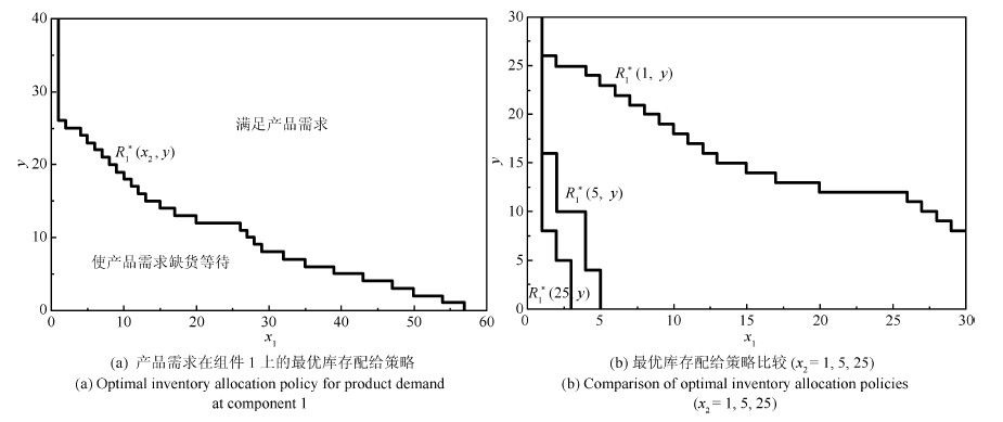 图 2 ATO系统产品需求的最优库存配给策略Fig. 2 Optimal inventory allocation policy for product demand in ATO
结论 4. 双需求型ATO系统,任一独立组件需求的库存配给值随系统内其他组件库存和产品需求缺货量的增加而增加.
图 3反映了独立组件1需求的最优配给策略.与图 2分析思路类似,图 3 (a)展示了在固定$x_{2}$情况下最优的库存配给策略.最优库存配给值$r^{\ast}_{1}$把状态空间分割成2个区域,当$x_{1}\geq r^{\ast}_{1}$时,满足独立组件需求为最优策略;反之,当$x_{1}< r^{\ast}_{1}$时,拒绝独立组件需求为最优策略.图 3(b) 清晰地展示了$r^{\ast}_{1}$随$x_{2}$与$y$的增加而增加的变化趋势.图 3的结论恰与图 2反映地产品需求的库存配给值变化规律相反.这一现象说明在ATO系统中,产品需求的优先级别高于独立组件需求.因为在实际大规模生产制造业中,最终产品的价格会远远高于组件的价格.独立组件只是作为产品的配件或者替换件出售,与产品相比其价格与需求量均较低.从经济利益角度,ATO型企业会倾向优先满足客户对产品的需求.当产品需求缺货量增加时,由于缺货的压力系统需要生产更多的组件充实库存装配产品,满足客户需求.在此情况下,独立组件需求将更难满足,因此其库存配给值升高.
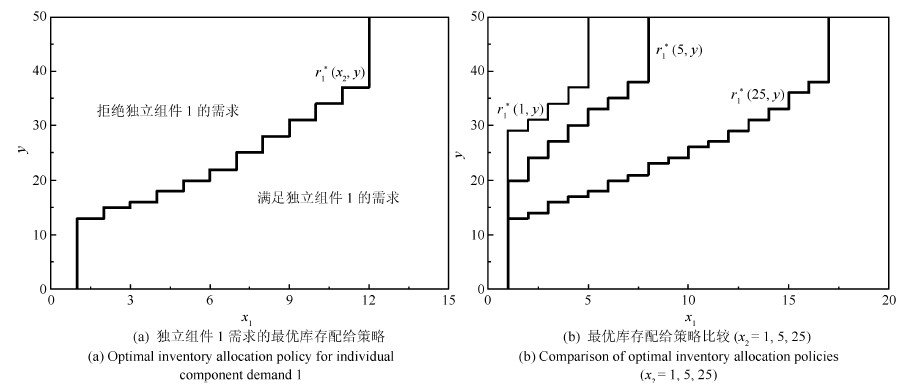 图 3 ATO系统独立组件需求最优库存配给策略Fig. 3 Optimal inventory allocation policy for individual component demand in ATO
3.2 启发式算法
本节提出启发式算法策略$H$.与最优策略相比,启发式算法策略的特点是具有确定的基础库存值.在算法$H$下,组件生产被确定型基础库存策略控制,产品需求和独立组件需求服从先到先服务(First-come-first-served,FCFS)准则.令$s_k$为组件$k$的确定型基础库存值,系统所有组件的确定型基础库存值为向量${s} = \left( {s_1 ,s_2 ,\cdots,s_n } \right)$.动态规划方程可以写为
$ \begin{matrix} {{v}^{*}}(x,y)=h(x)+{{b}_{0}}(y)+{{\lambda }_{0}}{{F}^{H,0}}{{v}^{*}}(x,y)+ \\ \sum\limits_{k=1}^{n}{{{\lambda }_{k}}{{F}^{H,k}}{{v}^{*}}(x,y)}+ \\ \sum\limits_{k=1}^{n}{{{\mu }_{k}}F_{k}^{H}{{v}^{*}}(x,y)} \\ \end{matrix} $
(4) $ {{F}^{H,0}}v(x,y)=\left\{ \begin{array}{*{35}{l}} v(x,y+1),\qquad \ \text{若}\underset{k=1}{\overset{n}{\mathop{\Pi }}}\,{{x}_{k}}=0 \\ v(x-e,y),\qquad \ \text{或} \\ \end{array} \right. $
$ {{F}^{H,k}}v(x,y)=\left\{ \begin{array}{*{35}{l}} v(x,y)+{{c}_{k}},\qquad 若\ {{x}_{k}}=0 \\ v(x-{{e}_{k}},y),\qquad \text{其他} \\ \end{array} \right. $
$ \begin{matrix} F_{k}^{H}v(x,y)= \\ ~\left\{ \begin{array}{*{35}{l}} v(x+{{e}_{k}},y), & \text{若}\ {{x}_{k}}<{{s}_{k}},y=0 & {} \\ v(x+{{e}_{k}},y), & \text{若}\ {{x}_{k}}<{{s}_{k}},y>0,\underset{i\ne k}{\overset{n}{\mathop{\Pi }}}\,{{x}_{i}}=0 & {} \\ v(x-\sum\limits_{i\ne k}^{n}{{{e}_{i}}},y-1)\}, & \text{若}\ y>0,\underset{i\ne k}{\overset{n}{\mathop{\Pi }}}\,{{x}_{i}}>0 & {} \\ v(x,y),\ \ \qquad \qquad \qquad & \text{其他} & {} \\ \end{array} \right. \\ \end{matrix} $
以2种组件3类需求的ATO系统为例,进行最优算法和启发式算法性能的比较分析.为得到更具一般性的结果,考虑一个相对广泛的组件生产参数范围(见表 1),计算最优策略和启发式算法策略的总折扣成本值.利用启发式策略成本$v^{H}$与最优成本$v^{\ast}$差值百分比$100%\times({v^{H}-v^{\ast}})/{v^{\ast}}$测量评价算法性能.可以看到,在测试例子中算法$H$总体的执行效果低于最优算法.在多数情况下缺货对系统的影响作用高于销售损失,系统处在严重缺货状态将导致销售损失和缺货等待并存.最优算法在独立组件需求和产品需求分配上有配给控制的优势,而配给策略的目的是把有用库存配给于价值更高的需求,从而达到组件库存在产品需求和组件需求间合理分配的目的.因此最优算法的执行效果高于启发式算法$H$.此外,算法$H$在独立组件需求到达率较高情况下(情况$2$,$7$,$9$,$18$,$20$,$24$,$26$)的执行效果相对较低.说明当独立组件需求水平提高时系统库存面临更高的缺货风险,最优算法可以利用动态基础库存值和配给水平值调节库存降低风险.而算法$H$没有确定的库存配给值调节库存分配,缺乏灵活性导致执行效果不显著.
表 1 最优策略vs.启发式算法策略Table 1 Optimal policy versus heuristics$\lambda_0$ $\lambda_1$ $ \lambda_2$ $\mu_1$ $\mu_2$ $h_1$ $h_2$ $b_0$ $c_1$ $c_2$ $\frac{({v^{H}-v^{\ast}})}{v^{\ast}}(\%)$ 1 1.05 0.43 1.71 2.43 3.06 5.90 4.63 82.17 117.63 276.33 1.574 2 0.60 1.03 2.45 2.98 3.42 5.59 4.96 69.88 227.82 454.58 5.734 3 1.32 2.60 1.07 3.84 3.22 4.82 4.60 47.74 182.11 199.48 1.371 4 1.70 2.46 2.37 4.95 3.97 5.76 6.74 92.02 310.57 405.30 2.429 5 0.26 5.19 1.66 4.55 3.36 3.51 4.47 86.85 483.11 384.78 3.099 6 0.79 1.81 1.98 4.57 3.18 2.02 5.49 66.18 209.95 332.79 0.686 7 0.69 1.65 1.96 2.63 4.95 6.84 6.69 52.93 427.26 386.80 6.115 8 0.26 3.79 2.59 3.46 3.20 2.16 8.58 69.10 480.45 197.10 0.243 9 1.97 1.04 0.42 4.81 4.01 1.69 5.66 54.73 200.01 164.37 5.052 10 1.59 2.79 1.45 3.80 3.97 6.80 6.55 83.89 277.30 173.66 1.627 11 0.46 1.84 1.63 2.67 1.92 8.07 7.27 49.97 352.29 277.87 1.169 12 0.78 1.88 3.19 4.20 3.99 1.49 7.46 93.58 348.68 465.15 0.185 13 1.01 1.07 1.94 2.57 3.80 3.84 3.57 51.64 297.04 144.26 2.873 14 0.30 0.24 1.31 0.72 2.68 9.42 9.15 40.28 142.12 356.00 0.604 15 1.14 2.47 0.69 4.69 3.54 4.65 7.08 108.09 388.54 305.73 4.842 16 1.42 0.77 6.51 2.44 9.82 8.56 3.66 74.49 318.02 219.48 1.798 17 0.04 4.73 2.18 5.82 2.16 1.47 9.61 210.47 458.20 143.43 2.829 18 1.30 1.38 7.43 4.35 9.46 4.92 2.30 178.88 155.86 188.07 5.380 19 2.16 1.91 4.31 4.96 7.81 5.03 5.83 93.49 365.78 443.31 1.373 20 1.00 7.47 8.12 9.57 8.10 5.47 1.47 155.48 220.94 353.92 4.670 21 2.67 4.58 2.88 8.30 8.02 6.85 5.54 135.60 198.65 492.38 1.830 22 2.36 7.22 2.05 9.95 4.97 7.44 2.72 83.86 100.10 296.27 1.096 23 0.34 7.99 7.54 7.64 7.75 2.13 7.06 206.66 421.96 331.71 1.182 24 1.23 2.41 9.73 6.79 9.50 2.21 3.22 204.06 369.70 195.20 6.379 25 1.20 2.77 3.61 5.97 7.51 9.05 4.40 213.99 474.80 100.03 2.233 26 1.56 6.87 6.54 9.02 8.31 8.58 6.56 166.86 227.97 371.99 11.512 27 0.54 8.36 2.54 9.54 5.38 1.26 1.68 119.78 305.63 255.31 0.126 28 1.50 4.37 9.17 6.43 9.95 2.05 1.90 127.34 393.21 390.50 2.209 29 1.71 6.67 2.80 7.16 8.61 9.97 3.28 103.01 277.92 410.01 1.778 30 1.09 9.29 6.05 9.81 7.01 3.85 9.17 160.18 493.08 439.47 1.207 (注: $\lambda_0 \sim {\rm U}(0,10)$, $\lambda_k \sim {\rm U}(0,10)$, $\mu_k \sim {\rm U}(1,10)$, $0.5 \le \rho _k \le 1.2$, $h_k \sim {\rm U}(1,10)$, $b_0 \sim {\rm U}(5,15) \times \sum\nolimits_{k = 1}^2 {h_k }$, $c_k \sim {\rm U}(100,500)$, }\\ \multicolumn{12}{l}{$\rho _k =\left( {\lambda _0 + \lambda _k } \right) / {\mu _k }$, $k = 1,2$.) 比较最优算法和启发式算法可以发现,最优算法是控制ATO系统组件生产-库存效果最好的一种策略方法.因为最优算法考虑到所有组件的基础库存和配给水平值,最优值可以控制组件的生产和库存分配.虽然启发式算法$H$缺乏动态控制系统库存的优势,但具有计算速度快、简单易操作的优点.因此算法$H$在优化控制ATO系统方面也是有效的,可以应用在生产实践中.
4. 结语
本文考虑实际产品市场上客户对产品及其独立组件的联合需求,研究了单一产品、多种组件装配的双需求型ATO系统的最优策略.系统含有销售损失和延期交货两种需求类型.在任一时间,对于任一组件,管理者必须做出生产决策:生产什么和生产多少.同时,对于任一需求到来,管理者还必须决定哪种需求可以满足.以上问题可以构建成一个MDP模型,应用动态规划方法求解.研究表明ATO系统组件的生产,产品需求和独立组件需求配给的最优策略均为状态依赖型,并以基础库存值和库存配给值来表示.在研究中得到了一些关于基础库存值和库存配给值的性质,以此来分析最优策略的结构特征.本文应用连续时间型MDP理论得到ATO系统的最优控制策略,有关最优策略的存在性与科学性已有大量学者进行相关论述,参见文献[2, 6-8, 13].通过仿真模拟实验进一步证明了最优策略的合理性,并得到了适合ATO型生产管理启示,为今后有效管理大型制造企业的生产与库存提供了新的理论依据.
致谢 在此特别感谢University of California Riverside,Riverside,USA美国加利福尼亚大学Mohsen ElHafsi教授,Ecole Centrale de Lille,France法国里尔中央理工大学Etienne Craye教授和Herve Camus教授对本文基础理论的指导.由衷感谢Mohsen ElHafsi教授对本文理论模型及定理定义的审议. -
图 2 ATO系统产品需求的最优库存配给策略
Fig. 2 Optimal inventory allocation policy for product demand in ATO
图 3 ATO系统独立组件需求最优库存配给策略
Fig. 3 Optimal inventory allocation policy for individual component demand in ATO
表 1 最优策略vs.启发式算法策略
Table 1 Optimal policy versus heuristics
$\lambda_0$ $\lambda_1$ $ \lambda_2$ $\mu_1$ $\mu_2$ $h_1$ $h_2$ $b_0$ $c_1$ $c_2$ $\frac{({v^{H}-v^{\ast}})}{v^{\ast}}(\%)$ 1 1.05 0.43 1.71 2.43 3.06 5.90 4.63 82.17 117.63 276.33 1.574 2 0.60 1.03 2.45 2.98 3.42 5.59 4.96 69.88 227.82 454.58 5.734 3 1.32 2.60 1.07 3.84 3.22 4.82 4.60 47.74 182.11 199.48 1.371 4 1.70 2.46 2.37 4.95 3.97 5.76 6.74 92.02 310.57 405.30 2.429 5 0.26 5.19 1.66 4.55 3.36 3.51 4.47 86.85 483.11 384.78 3.099 6 0.79 1.81 1.98 4.57 3.18 2.02 5.49 66.18 209.95 332.79 0.686 7 0.69 1.65 1.96 2.63 4.95 6.84 6.69 52.93 427.26 386.80 6.115 8 0.26 3.79 2.59 3.46 3.20 2.16 8.58 69.10 480.45 197.10 0.243 9 1.97 1.04 0.42 4.81 4.01 1.69 5.66 54.73 200.01 164.37 5.052 10 1.59 2.79 1.45 3.80 3.97 6.80 6.55 83.89 277.30 173.66 1.627 11 0.46 1.84 1.63 2.67 1.92 8.07 7.27 49.97 352.29 277.87 1.169 12 0.78 1.88 3.19 4.20 3.99 1.49 7.46 93.58 348.68 465.15 0.185 13 1.01 1.07 1.94 2.57 3.80 3.84 3.57 51.64 297.04 144.26 2.873 14 0.30 0.24 1.31 0.72 2.68 9.42 9.15 40.28 142.12 356.00 0.604 15 1.14 2.47 0.69 4.69 3.54 4.65 7.08 108.09 388.54 305.73 4.842 16 1.42 0.77 6.51 2.44 9.82 8.56 3.66 74.49 318.02 219.48 1.798 17 0.04 4.73 2.18 5.82 2.16 1.47 9.61 210.47 458.20 143.43 2.829 18 1.30 1.38 7.43 4.35 9.46 4.92 2.30 178.88 155.86 188.07 5.380 19 2.16 1.91 4.31 4.96 7.81 5.03 5.83 93.49 365.78 443.31 1.373 20 1.00 7.47 8.12 9.57 8.10 5.47 1.47 155.48 220.94 353.92 4.670 21 2.67 4.58 2.88 8.30 8.02 6.85 5.54 135.60 198.65 492.38 1.830 22 2.36 7.22 2.05 9.95 4.97 7.44 2.72 83.86 100.10 296.27 1.096 23 0.34 7.99 7.54 7.64 7.75 2.13 7.06 206.66 421.96 331.71 1.182 24 1.23 2.41 9.73 6.79 9.50 2.21 3.22 204.06 369.70 195.20 6.379 25 1.20 2.77 3.61 5.97 7.51 9.05 4.40 213.99 474.80 100.03 2.233 26 1.56 6.87 6.54 9.02 8.31 8.58 6.56 166.86 227.97 371.99 11.512 27 0.54 8.36 2.54 9.54 5.38 1.26 1.68 119.78 305.63 255.31 0.126 28 1.50 4.37 9.17 6.43 9.95 2.05 1.90 127.34 393.21 390.50 2.209 29 1.71 6.67 2.80 7.16 8.61 9.97 3.28 103.01 277.92 410.01 1.778 30 1.09 9.29 6.05 9.81 7.01 3.85 9.17 160.18 493.08 439.47 1.207 (注: $\lambda_0 \sim {\rm U}(0,10)$, $\lambda_k \sim {\rm U}(0,10)$, $\mu_k \sim {\rm U}(1,10)$, $0.5 \le \rho _k \le 1.2$, $h_k \sim {\rm U}(1,10)$, $b_0 \sim {\rm U}(5,15) \times \sum\nolimits_{k = 1}^2 {h_k }$, $c_k \sim {\rm U}(100,500)$, }\\ \multicolumn{12}{l}{$\rho _k =\left( {\lambda _0 + \lambda _k } \right) / {\mu _k }$, $k = 1,2$.)  下载: 导出CSV
-
[1] Song J S, Zipkin P. Supply chain operations: assemble-to-order systems, Chapter 11 in handbooks in operations research and management science. Supply Chain Management, 2003, 11(1): 561-596 [2] De Véricourt F, Karaesmen F, Dallery Y. Optimal stock allocation for a capacitated supply system. Management Science, 2002, 48(11): 1486-1501 [3] Karaarslan A G, Kiesmüller G P, De Kok A G. Analysis of an assemble-to-order system with different review periods. International Journal of Production Economics, 2013, 143(2): 335-341 [4] Saidane S, Babai M Z, Aguir M S, Korbaa O. On the performance of the base-stock inventory system under a compound erlang demand distribution. Computers & Industrial Engineering, 2013, 66(3): 548-554 [5] Juan A A, Grasman S E, Cáceres-Cruz J, Bektas T. A simheuristic algorithm for the single-period stochastic inventory-routing problem with stock-outs. Simulation Modelling Practice and Theory, 2014, 46: 40-52 [6] Benjaafar S, ElHafsi M. Production and inventory control of a single product assemble-to-order system with multiple customer classes. Management Science, 2006, 52(12): 1896-1912 [7] ElHafsi M, Li Z, Camus H, Craye E. An assemble-to-order system with product and components demand with lost sales. International Journal of Production Research, 2015, 53(3): 718-735 [8] 娄山佐, 田新诚. 随机供应中断和退货环境下库存问题的建模与控制. 自动化学报, 2014, 40(11): 2436-2443Lou Shan-Zuo, Tian Xin-Cheng. Modeling and control for inventory with stochastic supply disruptions and returns. Acta Automatica Sinica, 2014, 40(11): 2436-2443 [9] 娄山佐, 田新诚. 随机供应中断和退货环境下库存的应急控制. 自动化学报, 2015, 41(1): 94-103Lou Shan-Zuo, Tian Xin-Cheng. Contingent control of inventory under stochastic supply disruptions and returns. Acta Automatica Sinica, 2015, 41(1): 94-103 [10] 郭佳, 傅科, 陈功玉. 可变产能的按订单装配系统库存和生产决策研究. 中国管理科学, 2012, 20(3): 94-103Guo Jia, Fu Ke, Chen Gong-Yu. Optimal inventory and production decisions for an ATO system with variable capacity. Chinese Journal of Management Science, 2012, 20(3): 94-103 [11] 刘艳梅, 任佳, 江支柱, 刘曦泽, 祁国宁. 大批量定制下按订单装配产品同步生产计划方法. 计算机集成制造系统, 2014, 20(6): 1352-1358Liu Yan-Mei, Ren-Jia, Jiang Zhi-Zhu, Liu Xi-Ze, Qi Guo-Ning. Synchronized production planning method for assemble to order products of mass customization. Computer Integrated Manufacturing Systems, 2014, 20(6): 1352-1358 [12] Kim B, Kim J. A single server queue with Markov modulated service rates and impatient customers. Performance Evaluation, 2015, 83-84: 1-15 [13] Puterman M L. Markov Decision Processes: Discrete Stochastic Dynamic Programming. New York: John Wiley and Sons, 1994. 158-164 [14] Lippman S A. Applying a new device in the optimization of exponential queuing systems. Operations Research, 1975, 23(4): 687-710 期刊类型引用(1)
1. 苏兆品,李沫晗,张国富,刘扬. 基于Q学习的受灾路网抢修队调度问题建模与求解. 自动化学报. 2020(07): 1467-1478 .  本站查看
本站查看其他类型引用(11)
-

 下载:
下载:

计量
- 文章访问数: 2301
- HTML全文浏览量: 388
- PDF下载量: 886
- 被引次数: 12
