

-
摘要: 基于深度神经网络(Deep neutral networks, DNN)的分类方法因缺乏可解释性, 导致在金融、医疗、法律等关键领域难以获得完全信任, 极大限制了其应用. 现有多数研究主要关注单模态数据的可解释性, 多模态数据的可解释性方面仍存在挑战. 为解决这一问题, 提出一种基于视觉属性的多模态可解释图像分类方法, 该方法将可见光和深度图等不同视觉模态提取的属性融入模型的训练过程, 不仅能通过视觉属性和决策树对已有的神经网络黑盒模型进行解释, 而且能在训练过程中进一步提升模型解释信息的能力. 引入可解释性通常会造成模型精度的降低, 该方法在保持模型具有良好可解释性的同时, 仍具有较高的分类精度, 在NYUDv2、SUN RGB-D和RGB-NIR三个数据集上, 相比于单模态可解释方法, 该模型准确率明显提升, 并达到与多模态不可解释模型相媲美的性能.Abstract: The classification methods based on deep neutral networks (DNN) lack interpretability, which makes it difficult to gain complete trust in key fields such as finance, medical treatment, and law, greatly limiting their applications. Most existing research mainly focuses on the interpretability of uni-modal data, while there are still challenges in the interpretability of multimodal data. To address this issue, a multimodal interpretable image classification method based on visual attributes is proposed. This method incorporates attributes extracted from different visual modalities such as visible light and depth maps into the training process of the model. It not only interpret the existing black box model of neural networks through visual attributes and decision trees, but also further enhances the model's ability to interpret information during the training process. Introducing interpretability often leads to a decrease in model accuracy. This method maintains good interpretability while still maintaining high classification accuracy. Compared to uni-modal interpretable methods, the accuracy of this model is significantly improved on the NYUDv2, SUN RGB-D, and RGB-NIR datasets, and it achieves performance comparable to multi-modal uninterpretable models.
-
Key words:
- Interpretability /
- visual attributes /
- multimodal fusion /
- decision tree /
- image classification
-
驾驶员模型本质上即智能车辆的自动驾驶控制器, 自动完成车辆在特定驾驶任务下的速度控制与转向. 通常根据车辆运动的维度, 驾驶员模型可以大致分为纵向驾驶员模型、横向驾驶员模型与复合驾驶员模型[1]. 现如今最优控制理论、自适应控制理论与模型预测控制(Model predictive control, MPC)理论已成为当前驾驶员建模的主流方法. 如Yoshida等[2]采取自适应控制理论建立驾驶员模型. Qu等[3-4]提出了基于随机模型预测控制的驾驶员建模方法. Falcone等[5]则利用线性时变模型预测控制算法建立了自动驾驶车辆的转向控制器, 也可认为是横向驾驶员模型. Du等[6]利用非线性模型预测控制(Nonlinear model predictive control, NMPC)实现车辆速度和转向的综合控制. 未来随着人工智能技术的推进, 基于机器学习技术在特定驾驶任务条件下建立驾驶员模型也逐渐引起了人们的重视. 如Amsalu等[7]利用支持向量机对驾驶员在十字路口处的驾驶行为进行了分析与建模, 对驾驶员在十字路口的行为进行准确的预测, 并用于指导实际驾驶行为.
在智能驾驶员模型飞速发展的同时, 车辆的主动安全也逐渐引起了人们的重视[8]. 车辆的横向运动过程中主要面对的安全威胁包括: 1)在车辆转向过程中, 由于车辆系统的非线性和耦合性使其在高速、弯道或者在湿滑路面下极容易发生侧滑、侧翻、车道偏离等危险. 2)在复杂交通环境中, 因对交通场景中环境态势分析的不足, 导致和其他交通车辆发生碰撞事故.
本文研究的智能驾驶员模型主要解决两方面问题: 1)针对高速、低路面附着系数以及转弯工况下, 通过设计模型预测控制器作为车辆转向控制器并考虑车辆的侧向加速度、横摆角速度、质心侧偏角和横向转移率等现实约束, 实现智能车辆在跟踪轨迹的同时提高侧向稳定. 这里所指的侧向稳定性即车辆在行驶过程中, 不发生侧滑或侧翻的极限性能, 提高侧向稳定性即减小车辆发生侧滑、侧翻的风险. 2)在直线多车道的道路条件下, 通过分析一般工况下车辆换道行驶条件, 采用线性模型预测理论设计速度调整控制算法, 采用粒子群算法结合贝塞尔曲线设计轨迹发生器, 辅助智能车安全的实现自动换道的驾驶任务, 即在换道过程中不与环境车辆发生任意形式的碰撞.
1. 智能驾驶员模型结构
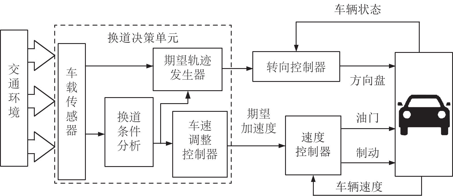
人类驾驶车辆的本质, 从控制系统的角度出发, 可看做是人—车—路环境构成的闭环系统. 人类驾驶员通过分析交通环境, 通过大脑制定出车辆应行驶的速度和轨迹, 并驱动方向盘和踏板执行相应的驾驶任务. 这一系列流程可概括为驾驶员的感知、决策和执行. 介于驾驶员具有以上特征, 本文设计的在换道条件下的驾驶员模型结构如图1所示.
在该结构中, 驾驶员模型可划分为换道决策单元、转向控制器模块和速度控制器用来实现换道任务. 换道决策单元将结合具体车道环境, 合理分析换道条件、规划期望行驶的轨迹和车速避免事故的发生. 期望轨迹和车速信号作用于下游的转向控制器和速度控制器完成具体的转向和速度操控. 其中, 本方案中的速度控制器根据现有成果, 采用模糊神经网络算法计算指定工况下油门开度和制动压强实现对汽车加速度的控制[9]. 而转向控制器的设计, 保证轨迹跟踪精度的同时必须兼顾车辆自身的侧向稳定性. 这里所说的侧向稳定性指标包括质心侧偏角、横摆角速度、侧向加速度和横向转移率. 因此, 转向控制器的设计本质上是以轨迹跟踪精度为控制目标, 以方向盘转角为控制量, 同时兼顾汽车质心侧偏角、横摆角速度、侧向加速度和横向转移率等稳定性约束的, 具有多目标多约束的最优控制求解问题[10]. 下面将分别就本驾驶员模型中的转向控制器以及决策规划模块的详细内容进行说明.
2. 转向控制器设计
2.1 车辆动力学模型
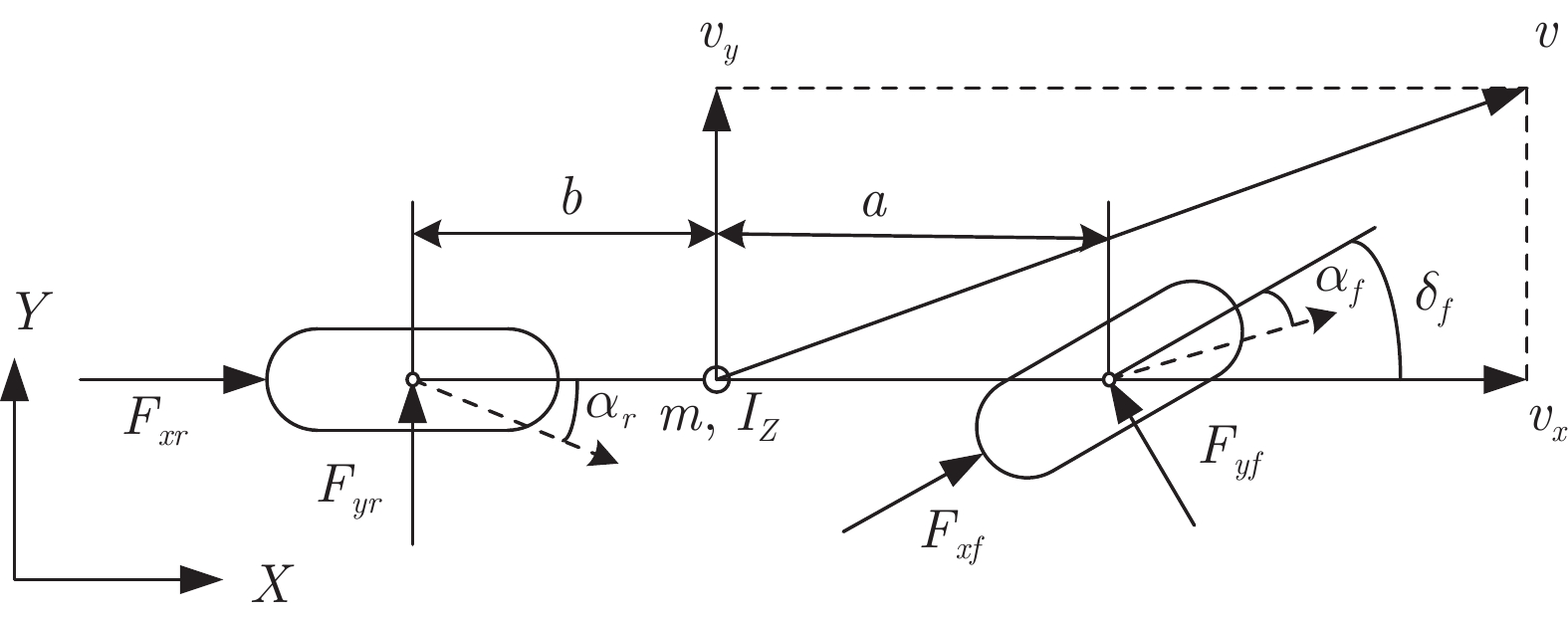
利用模型预测控制理论进行转向控制器的设计, 需要对被控对象进行清晰准确的描述. 本文选取两轮三自由度的非线性车辆动力学模型作为转向控制器设计的依据. 假设车辆在行驶过程中前轮转角与方向盘转角之间的传动比为线性关系, 且两个前轮的转向角度一致. 同时忽略车辆垂直与俯仰运动, 忽略空气动力学、侧向风与轮胎回正力矩对车身的作用. 模型结构如图2所示.
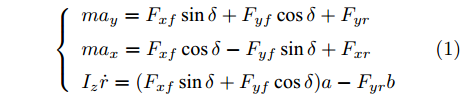
通过对车辆模型的纵向、侧向、横摆和侧倾运动的受力分析, 可以推导出其动力学方程为
$$ \left\{ {\begin{array}{*{20}{l}} {m{a_y} = {F_{xf}}\sin \delta + {F_{yf}}\cos \delta + {F_{yr}}}\\ {m{a_x} = {F_{xf}}\cos \delta - {F_{yf}}\sin \delta + {F_{xr}}}\\ {{I_z}\dot r = ({F_{xf}}\sin \delta + {F_{yf}}\cos \delta )a - {F_{yr}}b} \end{array}} \right. $$ (1) 图2中的各个参数分别表示如下:
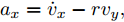
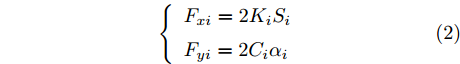
$ a_x $ 为车辆的纵向加速度$({\rm{m/s}}^2)$ ;$ a_y $ 为车辆的侧向加速度$({\rm{m/s}}^2)$ ;$ \psi $ 为车辆横摆角$({\rm{rad}})$ ;$ r $ 为车辆的横摆角速度$({\rm{rad/s}})$ ;$ \delta $ 是汽车前轮转角$({\rm{rad}})$ , 其与方向盘转角$ {\delta _{sw}} $ 之间的线性系数$ G $ ;$ m $ 是车辆的整体质量$({\rm{kg}})$ ;$ I_z $ 代表车辆$ z $ 轴的转动惯量$({\rm{kg/m}}^2)$ .$ a $ 和$ b $ 分别为质心到车轮前后轴的轴距$({\rm{m}})$ . 通常,${a_x} = {{\dot v}_x} - r{v_y},\;$ ${a_y} = $ $ {{\dot v}_y} - r{v_x}.\;$ $ v_x $ 和$ v_y $ 是车相对自身纵轴和横轴的速度$({\rm{m/s}}).\;$ 轮胎所受的纵向力$ F_{xi} $ 与侧向力$ F_{yi}(N) $ 由路面提供, 通常在滑移率和轮胎侧偏角较小的情况下, 其可近似为$$ \left\{ \begin{array}{l} {F_{xi}} = 2{K_i}{S_i}\\ {F_{yi}} = 2{C_i}{\alpha _i} \end{array} \right. $$ (2) 式中,
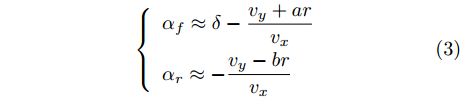
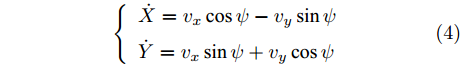
$i = f ,\;$ $ r $ .$ K_i $ 与$ C_i $ 分别为轮胎的纵向刚度与侧向刚度$({\rm{N/m}})$ ,$ S_i $ 为轮胎滑移率, 是一无量纲参数, 通常在车辆匀速行驶中可近似为一个定值, 本文定义为$0.2 .$ 轮胎侧偏角$\alpha_i\;({\rm{rad}})$ 则满足$$ \left\{ \begin{array}{l} {\alpha _f} \approx \delta - \dfrac{{{v_y} + ar}}{{{v_x}}}\\ {\alpha _r} \approx - \dfrac{{{v_y} - br}}{{{v_x}}} \end{array} \right. $$ (3) 此外, 车辆在运动过程中, 车辆在大地坐标系下的位移可表示为
$$ \left\{ \begin{array}{l} \dot X = {v_x}\cos \psi - {v_y}\sin \psi \\ \dot Y = {v_x}\sin \psi + {v_y}\cos \psi \end{array} \right. $$ (4) 式中,
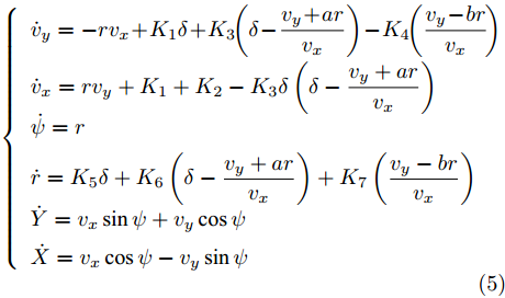
$ X $ 与$ Y $ 分别为车辆相对于地面的纵向与侧向位移$ (m) $ . 在转向控制器的设计中, 通常需要将复杂的车辆动力学方程简化. 实际转向中车辆前轮转角$ \delta $ 满足$ \cos \delta \approx 1 $ ,$ \sin \delta \approx \delta $ . 因此, 车辆系统状态空间表达式[11]为$$ \left\{ \begin{array}{l} {{\dot v}_y} = - r{v_x} \!+\! {K_1}\delta \!+\! {K_3}\!\!\left(\delta \!-\! \dfrac{{{v_y} \!+\! ar}}{{{v_x}}}\right) \!-\! {K_4}\!\!\left(\dfrac{{{v_y} \!-\! br}}{{{v_x}}}\!\right)\\ {{\dot v}_x} = r{v_y} + {K_1} + {K_2} - {K_3}\delta \left(\delta - \dfrac{{{v_y} + ar}}{{{v_x}}}\right)\\ \dot \psi = r\\ \dot r = {K_5}\delta + {K_6}\left(\delta - \dfrac{{{v_y} + ar}}{{{v_x}}}\right) + {K_7}\left(\dfrac{{{v_y} - br}}{{{v_x}}}\right)\\ \dot Y = {v_x}\sin \psi + {v_y}\cos \psi \\ \dot X = {v_x}\cos \psi - {v_y}\sin \psi \end{array} \right. $$ (5) 其中,
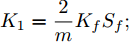
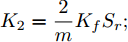
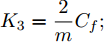
${K_1} = \dfrac{2}{m}{K_f}{S_f};\;$ ${K_2} = \dfrac{2}{m}{K_f}{S_r};\;$ ${K_3} = \dfrac{2}{m}{C_f};\;$ ${K_4} = \dfrac{2}{m}{C_r} ;\;$ ${K_5} = \dfrac{2}{{{I_z}}}a{K_f}{S_f};\;$ ${K_6} = \dfrac{2}{{{I_z}}}a{C_f};\;$ ${K_7} = $ $ \dfrac{2}{{{I_z}}}{C_r}b.\;$ 定义系统状态变量
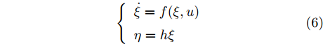
$ \xi $ 为:$v_y ,\;$ $v_x ,\;$ $\psi ,\;$ $r ,\;$ $Y ,\;$ $ X .$ 定义前轮转角$ \delta $ 为控制量$u .\;$ 车辆的侧向位移与巡航角为系统的被控变量$ \eta $ , 因此上述连续控制系统的状态空间方程可以表示为$$ \left\{ \begin{array}{l} \dot \xi = f(\xi ,u)\\ \eta = h\xi \end{array} \right. $$ (6) 式中, 矩阵
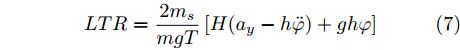
${{h}}$ 为系统输出矩阵.衡量车辆侧倾稳定性的性能指标通常取车辆横向转移率(Lateral transfer rate, LTR), 其原理如图3所示. 图中的各个参数分别为:
$ g $ 代表重力加速度$({\rm{m/s}}^2)$ ,$ \varphi $ 是车辆的侧倾角度$({\rm{rad}})$ ,$ m_s $ 是车辆簧载质量$({\rm{kg}})$ ,$ I_x $ 是车辆x轴的转动惯量$({\rm{kg/m}}^2)$ .$ h $ 为侧倾臂长$({\rm{m}})$ ,$ H $ 代表簧载质心距离地面的高度$({\rm{m}})$ ,$ T $ 表示车辆宽度$({\rm{m}})$ . 其大小与车辆侧向加速度、侧倾角、侧倾角加速度相关, 指标形式如下[12]:$$ LTR = \dfrac{{2{m_s}}}{{mgT}}\left[ {H({a_y} - h\ddot \varphi ) + gh\varphi } \right] $$ (7) 2.2 转向控制系统设计
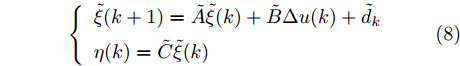
本文中, 转向控制器设计采用线性时变模型预测控制理论, 该控制器需要对预测模型、目标函数和约束条件进行设计[13]. 连续系统的状态空间表达式, 经线性化、离散化和增量化后的结果为
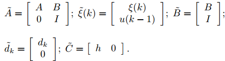
$$ \left\{ \begin{array}{l} \tilde \xi (k + 1) = \tilde A\tilde \xi (k) + \tilde B\Delta u(k) + {{\tilde d}_k}\\ \eta (k) = \tilde C\tilde \xi (k) \end{array} \right. $$ (8) 式中,
$$ \begin{split} &\tilde A = \left[ {\begin{array}{*{20}{c}}A&B\\0&I\end{array}} \right] \!; \;\tilde \xi (k) = \left[ {\begin{array}{*{20}{c}}{\xi (k)}\\{u(k - 1)}\end{array}} \right]\! ;\; \tilde B = \left[ {\begin{array}{*{20}{c}}B\\I\end{array}} \right]\! ; \\ & {\tilde d_k} = \left[ {\begin{array}{*{20}{c}}{{d_k}}\\0\end{array}} \right]\! ; \;\tilde C = \left[ {\begin{array}{*{20}{c}}h&0\end{array}} \right]. \end{split} $$ 其中,
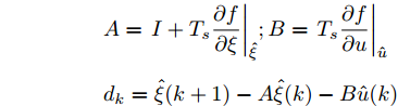
${{I}}$ 为单位矩阵, 其他各个符号的含义为$$ \begin{split} &A = {\left. {I + {T_s}\dfrac{{\partial f}}{{\partial \xi }}} \right|_{\hat \xi }} ; B = {\left. {{T_s}\dfrac{{\partial f}}{{\partial u}}} \right|_{\hat u}} \\ &{d_k} = \hat \xi (k + 1) - A\hat \xi (k) - B\hat u(k) \end{split} $$ 上述各式中,
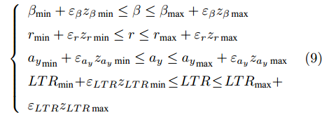
$ T_s $ 定义为离散系统采样时间,$ \hat \xi $ 和$ \hat u $ 为当前系统的状态量和控制量.由于转向控制系统的主要控制目标是保证轨迹跟踪精度并同时兼顾车辆的侧向稳定性. 因此本文将其转化为轨迹控制精度的性能指标以及对车辆主要状态的约束的形式. 系统的主要侧向约束指标包括质心侧偏角、横摆角速度、侧向加速度和横向转移率, 其具体形式为
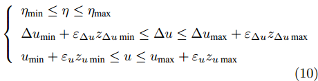
$$ \left\{ {\begin{array}{*{20}{l}} {{\beta _{\min }} + {\varepsilon _\beta }{z_{\beta \min }} \le \beta \le {\beta _{\max }} + {\varepsilon _\beta }{z_{\beta \max }}}\\ {{r_{\min }} + {\varepsilon _r}{z_{r\min }} \le r \le {r_{\max }} + {\varepsilon _r}{z_{r\max }}}\\ {{a_y}_{\min } + {\varepsilon _{{a_y}}}{z_{{a_y}\min }} \le {a_y} \le {a_y}_{\max } + {\varepsilon _{{a_y}}}{z_{{a_y}\max }}}\\ {LT{R_{\min }} \!+\! {\varepsilon _{LTR}}{z_{LTR\min }} \!\le\! LTR \!\le\! LT{R_{\max }}}+\\ { {\varepsilon _{LTR}}{z_{LTR\max }}} \end{array}} \right. $$ (9) 考虑车辆系统的实际运动极限, 转向控制系统输出量、控制增量和控制量也应满足约束
$$ \left\{ \begin{array}{l} {\eta _{\min }} \le \eta \le {\eta _{\max }}\\ \Delta {u_{\min }} + {\varepsilon _{\Delta u}}{z_{\Delta u\min }} \le \Delta u \le \Delta {u_{\max }} + {\varepsilon _{\Delta u}}{z_{\Delta u\max }}\\ {u_{\min }} + {\varepsilon _u}{z_{u\min }} \le u \le {u_{\max }} + {\varepsilon _u}{z_{u\max }} \end{array} \right. $$ (10) 式中,
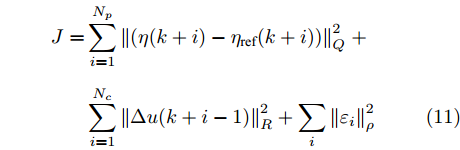
$ {\varepsilon _i} $ 为各个约束变量的松弛因子, 用于保证系统存在可行解. 为提高系统控制精度, 减小执行机构的运动幅度, 定义系统的性能指标为$$ \begin{split} J = & \displaystyle\sum\limits_{i = 1}^{{N_p}} {\left\| {(\eta (k + i) - {\eta _{{\rm{ref}}}}(k + i))} \right\|_Q^2} \;+\\ & \displaystyle\sum\limits_{i = 1}^{{N_c}} {\left\| {\Delta u(k + i - 1)} \displaystyle\right\|_R^2} + \displaystyle\sum\limits_i {\left\| {{\varepsilon _i}} \right\|_\rho ^2} \end{split} $$ (11) 式中,
$ N_p $ 为预测模型的预测时域,$ N_c $ 为预测模型的控制时域,$ {\eta _{{\rm{ref}}}} $ 为期望输出的侧向轨迹.$Q ,\;$ $ R $ 和$ \rho $ 代表相应的权重系数. 根据滚动优化理论, 系统状态方程在预测时域和控制时域内不断迭代后得到的系统预测模型, 结合性能指标与约束条件, 经二次规划算法可计算出最优控制序列$$ {u^*}(k) = {u^*}(k - 1) + \left[ {\begin{array}{*{20}{c}} 1&0& \cdots &0 \end{array}} \right]\Delta {U^*}(k) $$ (12) 根据方向盘与前轮转角的比例系数
$ G $ , 可计算出方向盘转角的最优解为$$ {u_{SW}}^*(k) = G{u^*}(k) $$ (13) 3. 换道决策系统设计
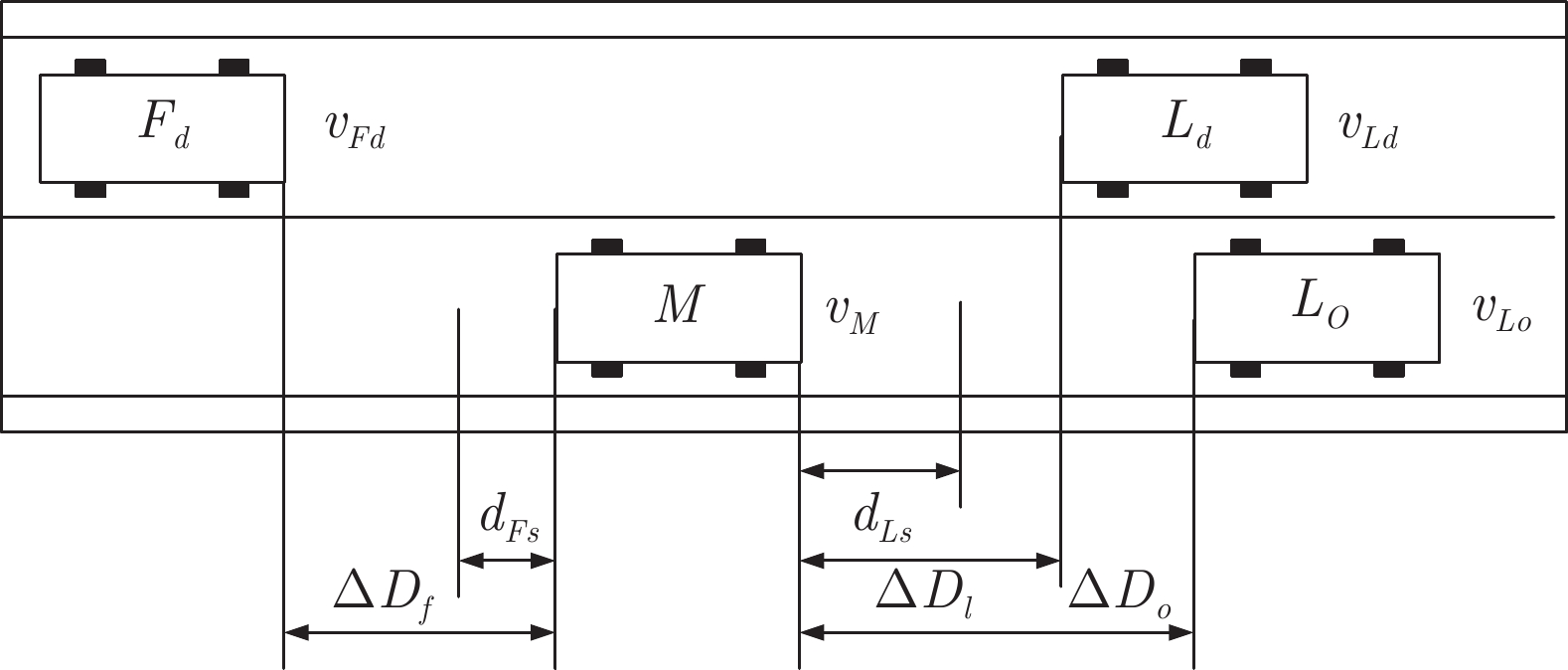
当车辆前方出现妨碍自身正常行驶的车辆或障碍物时, 为了提高驾驶效率, 人类驾驶员会通过变换车道的方式实现更好的驾驶体验[14]. 假设换道开始前交通车分布如图4所示.
在换道行驶过程中, 智能车M会因转向不足或安全间距过小导致和原车道前车(Lead vehicle of the original lane, Lo)发生追尾或斜向剐蹭. 或因车速调整不当或安全间距不足导致和目标车道的前车(Lead vehicle of the destined lane, Ld)和后车(Follow vehicle of the destined lane, Fd)发生追尾或剐蹭. 因此, 针对目标车道的换道行为, 本文将结合目标车道前后车的间距和速度情况做出分析, 计算出合理的行驶车速和跟车间距. 为避免因转向不足导致的与原车道前车相撞, 本驾驶员模型将结合前后两车的间距及其换道方向, 规划换道路径.
3.1 换道车辆安全性分析
根据图4中换道前车辆分布, 设
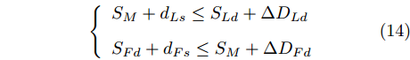
$ t_0 $ 为换道开始时刻,$\Delta {D_{Lo}} ,\;$ $\Delta {D_{Ld}},\;$ 和$\Delta {D_{Fd}}$ 分别为智能车$ M $ 与原车道前车、目标车道前车和后车的当前间距.$ d_{Ls} $ 为车辆$ M $ 与前车的期望安全间距,$d_{Fs}$ 为车辆$ M $ 与后车的期望安全间距.$ v_i $ 为环境中各车车速$(i = $ $ M,L_o,L_d,F_d)$ . 假设换道前后目标车道车辆的位置关系如图5所示.图中虚线代表换道前各个车辆所处的位置, 实线为换道结束后各车辆对应的位置,
$ S_i $ 为各车在换道期间行驶的路程. 通常为使换道结束后前后两车的车距仍处在驾驶员期望安全间距之外, 车辆行驶过程应满足$$ \left\{ \begin{array}{l} {S_M} + {d_{Ls}} \le {S_{Ld}} + \Delta {D_{Ld}}\\ {S_{Fd}} + {d_{Fs}} \le {S_M} + \Delta {D_{Fd}} \end{array} \right. $$ (14) 前车安全间距
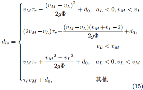
$d_{Ls}$ 通常根据前后两车车速$ v_M $ 与$ v_L $ 、路面附着系数$ \Phi $ 重力加速度$ g $ 和与车间最小安全间距$ d_0 $ 来确定, 其不同环境下的大小为[15]$$ {d_{ls}} = \left\{ \begin{aligned} &{v_M}{\tau _r} - \dfrac{{{{({v_M} - {v_L})}^2}}}{{2g\Phi }} + {d_0},\;\;{a_L} < 0,{v_M} < {v_L}\\ &(2{v_M} \!-\! {v_L}){\tau _r} \!+\! \dfrac{{({v_M} \!-\! {v_L})({v_M} \!+\! {v_L} \!-\! 2)}}{{2g\Phi }} \!+\! {d_0},\\ &\qquad\qquad\qquad\qquad\qquad\;\;\;\;\;\;\,{v_L} < {v_M}\\ &{v_M}{\tau _r} + \dfrac{{{v_M}^2 - {v_L}^2}}{{2g\Phi }} + {d_0},\;\;\;{a_L} < 0,{v_L} < {v_M}\\ &{\tau _r}{v_M} + {d_0},\qquad\qquad\qquad\quad\!{\text{其他}} \end{aligned} \right. $$ (15) 上式中
$ d_0 $ 的定义参阅文献[15], 其形式为$$ {d_0} = {d_{Fs}} = k\frac{c}{{\Phi + d}} $$ (16) 式中,
$ c $ 和$ d $ 为一常量, 在本文中定义$ c = 1.8 $ ,$ d = 0.17 $ .$ k $ 为反映驾驶员实际意图的系数.假设车辆M的加速度为a, 通常情况下, 车辆M当前所处的车流中各车车速可大致划分为:
工况1.
$ v_M $ $ > $ $ v_{Ld} $ $ > $ $v_{Fd},$ 此时目标车道车速低于自车车速, 智能车$ M $ 向目标车道减速换道行驶.工况2.
$ v_{Ld} $ $ > $ $ v_{Fd} $ $ > $ $v_M ,$ 此时智能车$ M $ 为了不与目标车道后车发生剐蹭, 需加速换道.工况3.
$ v_{Ld} $ $ > $ $ v_M $ $ > $ $v_{Fd},$ 此时智能车$ M $ 可以匀速或加速向目标车道换道行驶.定义驾驶员反应时间为
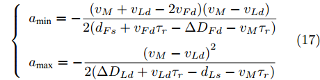
$ {{\tau _r}} $ . 根据式(14) 以及牛顿运动学公式分别计算出智能车$ M $ 在以上3种情况下换道过程中采取的加速度上下限, 即$a_{{\rm{min}}}$ 与$a_{{\rm{max}}}$ .工况1中, 当
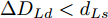
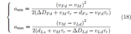
$\Delta {D_{Ld}} < {d_{Ls}}$ 时, 此时由于$L_d$ 车速慢于本车, 且两车间距已经小于安全间距, 换道会增大两车相撞风险, 所以此工况下不做换道操作. 相反, 若车间距关系满足$\Delta {D_{Ld}} \ge {d_{Ls}}$ , 根据式(14)可计算出车辆M的加速度上下限为$$ \left\{ \begin{array}{l} {a_{\min }} = - \dfrac{{({v_M} + {v_{Ld}} - 2{v_{Fd}})({v_M} - {v_{Ld}})}}{{2({d_{Fs}} + {v_{Fd}}{\tau _r} - \Delta {D_{Fd}} - {v_M}{\tau _r})}}\\ {a_{\max }} = - \dfrac{{{{({v_M} - {v_{Ld}})}^2}}}{{2(\Delta {D_{Ld}} + {v_{Ld}}{\tau _r} - {d_{Ls}} - {v_M}{\tau _r})}} \end{array} \right. $$ (17) 在工况2中, 若此时换道时若车间距条件满足
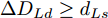
$\Delta {D_{Fd}} < {d_{Fs}}$ , 由于目标车道后车车速较快且两车距离已经小于二者的安全间距, 因此不做换道. 相反, 若$\Delta {D_{Fd}} \ge {d_{Fs}}$ 且$\Delta {D_{Ld}} < {d_{Ls}} ,\;$ 则$$ \left\{ \begin{array}{l} {a_{\min }} = \dfrac{{{{({v_{Fd}} - {v_M})}^2}}}{{2(\Delta {D_{Fd}} + {v_M}{\tau _r} - {d_{Fs}} - {v_{Fd}}{\tau _r})}}\\ {a_{\max }} = \dfrac{{{{({v_M} - {v_{Ld}})}^2}}}{{2({d_{Ls}} + {v_M}{\tau _r} - \Delta {D_{Ld}} - {v_{Ld}}{\tau _r})}} \end{array} \right.$$ (18) 若
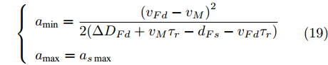
$\Delta {D_{Fd}} \ge {d_{Fs}}$ 且$\Delta {D_{Ld}} \ge {d_{Ls}}$ , 此时目标车道前车车速快于本车且两车间距已大于安全间距, 则车辆$ M $ 拟采取的加速度范围为$$ \left\{ \begin{array}{l} {a_{\min }} = \dfrac{{{{({v_{Fd}} - {v_M})}^2}}}{{2(\Delta {D_{Fd}} + {v_M}{\tau _r} - {d_{Fs}} - {v_{Fd}}{\tau _r})}}\\ {a_{\max }} = {a_{s\max }} \end{array} \right. $$ (19) 在工况3中, 由于此时目标车道后车慢于自车车速, 因此智能车
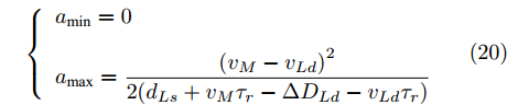
$ M $ 无需考虑与其发生碰撞, 只考虑与前车的安全间距. 若$\Delta {D_{Ld}} < {d_{Ls}} ,\;$ 加速度范围满足:$$ \left\{ \begin{array}{l} {a_{\min }} = 0\\ {a_{\max }} = \dfrac{{{{({v_M} - {v_{Ld}})}^2}}}{{2({d_{Ls}} + {v_M}{\tau _r} - \Delta {D_{Ld}} - {v_{Ld}}{\tau _r})}} \end{array} \right. $$ (20) 相反, 若满足
$\Delta {D_{Ld}} \ge {d_{Ls}} ,\;$ 加速度范围为$$ \left\{ \begin{array}{l} {a_{\min }} = 0\\ {a_{\max }} = {a_{s\max }} \end{array} \right. $$ (21) 通常人类驾驶车辆过程中, 车辆实际行驶的极限加速度范围为:
$ a \in [{a_{s\min }},{a_{s\max }}] $ , 此处$a_{s{\rm{min}}}$ 与$a_{s{\rm{max}}}$ 是在保证车辆与驾驶员的舒适与稳定条件下加速度最小值与最大值. 将前文所述的安全换道加速范围与舒适性范围取交集, 即为本文设计驾驶员换道模型应采取的加速范围, 当分析模块计算出此范围为非空集合时, 代表当前工况下换道存在可行性, 即车速调整模块实际采取的加速区间为$$ u \in [{u_{\min }},{u_{\max }}] = [{a_{s\min }},{a_{s\max }}] \cap [{a_{\min }},{a_{\max }}] $$ (22) 3.2 车速调整控制系统设计
通常, 驾驶员在驶入与
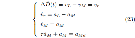
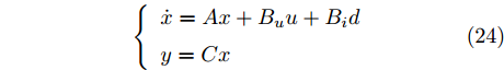
$L_o$ 的安全间距之内, 首先要根据$L_o$ 的运动状态调整两车的间距和速度关系, 并同时判断目标车道是否存在换道空间, 当换道空间达成后以目标车道前车为跟车对象进行车速和轨迹的调整. 因此在本驾驶员模型车速调整控制中, 将以前后两车的运动关系为被控对象进行调整. 在实际车辆行驶过程中, 前后两车间距$ \Delta D $ 、速度差$ v_r $ 、前后车车速$ v_L $ 与$ v_M $ , 前后车加速度$ a_L $ 和$ a_M $ , 后车期望加速度$ a_{Md} $ 之间满足$$ \left\{ \begin{array}{l} \mathop {\Delta {\dot D}(t)} = {v_L} - {v_M} = {v_r}\\ {{{\dot v}_r}} = {a_L} - {a_M}\\ {{\dot v}_M} = {a_M}\\ \tau {{{\dot a}_M}} + {a_M} = {a_{Md}} \end{array} \right. $$ (23) 将上式转换为状态空间表达式形式, 定义状态量
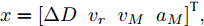
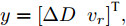
$x = {\left[ {\Delta D}\;\;{{v_r}}\;\;{{v_M}}\;\;{{a_M}} \right]^{\rm{T}}},$ 控制量$ u = a_{Md} $ , 扰动量$ d = a_L $ , 系统输出$y = {\left[ {\Delta D}\;\;{{v_r}} \right]^{\rm{T}}} ,$ 上述方程可表示为$$ \left\{ \begin{array}{l} \dot x = Ax + {B_u}u + {B_i}d\\ y = Cx \end{array} \right. $$ (24) 取采样周期
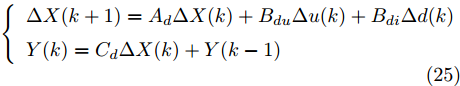
$ T $ , 取增量式进行算法设计, 因此系统离散化后结果为$$ \left\{ \begin{array}{l} \Delta X(k + 1) = {A_d}\Delta X(k) + {B_{du}}\Delta u(k) + {B_{di}}\Delta d(k)\\ Y(k) = {C_d}\Delta X(k) + Y(k - 1) \end{array} \right. $$ (25) 其中,
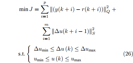
${A_d} \!=\! I + TA$ ,$B_{du} \!=\! TB_u ,\;$ $B_{di} \!=\! TB_i ,\;$ $ C_d = C $ . 同样采用滚动优化思想, 对状态方程在预测时域$ p $ 和控制时域$ m $ 内迭代出系统的预测方程. 为了满足所要达到的控制目标, 定义控制器的参考输入$r(k + i) = {\left[ {{D_{{\rm{des}}}}(k)}\;\;0 \right]^{\rm{T}}}$ , 其中$D_{{\rm{des}}}(k)$ 此处定义为期望安全间距$ d_{ls} $ , 期望两车速度差$ v_r $ 为0. 速度控制系统的性能指标与控制量约束为$$ \begin{split} &\min J = \displaystyle\sum\limits_{i = 1}^p {\left\| {(y(k + i) - r(k + i))} \right\|} _Q^2\;+\\ \begin{array}{*{20}{c}} {}&{} \end{array} &\qquad\qquad\displaystyle\sum\limits_{i = 1}^m {\left\| {\Delta u(k + i - 1)} \right\|} _S^2\\ &{\rm{s.t.}}\left\{ \begin{array}{l} \Delta {u_{\min }} \le \Delta u\left( k \right) \le \Delta {u_{\max }}\\ {u_{\min }} \le u\left( k \right) \le {u_{\max }} \end{array} \right. \end{split} $$ (26) 式中,
${{Q}}$ 和${{S}}$ 代表输出量与控制增量序列的权重矩阵. 同样利用二次规划算法计算出期望加速度的最优解$ a_{Md}^*(k) $ .3.3 期望轨迹发生器的设计
为避免因转向不足导致和前车
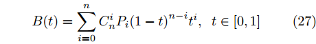
$L_o$ 的斜向剐蹭, 本驾驶员模型采用基于粒子群的贝塞尔曲线实施轨迹规划. 通常$ n $ 次贝塞尔曲线可表示为$$ B(t) = \sum\limits_{i = 0}^n {C_n^i{P_i}{{(1 - t)}^{n - i}}{t^i}} ,\;\;t \in [0,1] $$ (27) 其中,
$ P_i $ 为曲线的关键点坐标. 在轨迹规划中, 轨迹规划的关键点的选取方式如图6所示.图6显示了自车在换道开始前两车的位置关系. 设两车当前间距为
$\Delta {D_{Lo}}$ . 以实施左换道为例, 定义各个主要关键点的位置为: 实验车M的车头中心坐标$ {P_1}({x_1},{y_1}) $ , 前车左后点$ {P_6}({x_6},{y_6}) $ . 根据车辆轨迹的曲线特性, 在轨迹中距离前车$ P_6 $ 点最近的一点必为该轨迹切点$ {P_3}({x_3},{y_3}) $ . 定义两点间的距离为$ R $ ,$ R $ 也可看做是轨迹与前车间的最小距离.$ P_3 $ 同时也是以$ P_6 $ 为圆心的圆的外切点. 那么将$ P_3 $ 切线与两侧车道中心线的交点定义为$ {P_3}({x_3},{y_3}) $ 和$ {P_4}({x_4},{y_4}) $ . 而目标车道上位于$ P_4 $ 前方的任意一点被定义为$ {P_5}({x_5},{y_5}) $ .因此, 根据参考轨迹初步设置的5个关键点, 故可采用四次贝塞尔曲线来实现轨迹规划. 为使该参考轨迹更加平滑、均匀[16], 易于跟踪, 因此本文选取优化性能指标为
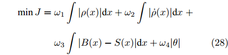
$$ \begin{split} \min J =\;& {\omega _1}\int {|\rho (x)|{\rm{d}}x} + {\omega _2}\int {|\dot \rho (x)|{\rm{d}}x}\; +\\ & {\omega _3}\int {|B(x) - S(x)|{\rm{d}}x} + {\omega _4}|\theta | \end{split} $$ (28) 式中,
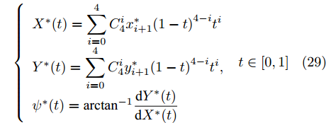
$ \rho (x) $ 与$ \dot \rho (x) $ 为贝塞尔曲线的曲率及其导数,$ B(x) $ 与$ S(x) $ 分别为贝塞尔曲线函数和结构线函数,$ \theta $ 为过$ P_3 $ 点的切线与$ x $ 轴的夹角. 而$ \omega _i $ 为各个性能指标的权系数. 为使性能指标尽快达到最优结果, 本文最终采用粒子群算法求解各个主要关键点的最优坐标$ P_i^*(x_i^*,y_i^*) $ , 最后根据贝塞尔曲线公式, 得出车辆换道过程的参考轨迹$$ \left\{ \begin{array}{l} {X^*}(t) = \displaystyle\sum\limits_{i = 0}^4 {C_4^ix_{i + 1}^*{{(1 - t)}^{4 - i}}{t^i}} \\ {Y^*}(t) = \displaystyle\sum\limits_{i = 0}^4 {C_4^iy_{i + 1}^*{{(1 - t)}^{4 - i}}{t^i}}, \\ {\psi ^*}(t) = {\arctan ^{ - 1}}\dfrac{{{\rm{d}}{Y^*}(t)}}{{{\rm{d}}{X^*}(t)}} \end{array} \right.\;t \in [0,1] $$ (29) 4. 智能驾驶系统实验验证
本智能驾驶员模型将在CarSim/Simulink仿真环境下, 分别就车辆在轨迹跟踪以及自主换道两种交通场景进行实验验证. 实验车辆为CarSim2016中的D-Class型轿车.
4.1 智能车轨迹跟踪与侧向稳定性验证
为验证本模型转向控制算法的可靠性, 本文分别对该驾驶员模型在高速、低路面附着系数以及弯道三种工况下驾驶员模型转向控制器进行验证. 分别对无约束模型预测控制器和本文采用的带约束模型预测控制器的控制效果进行对比说明.
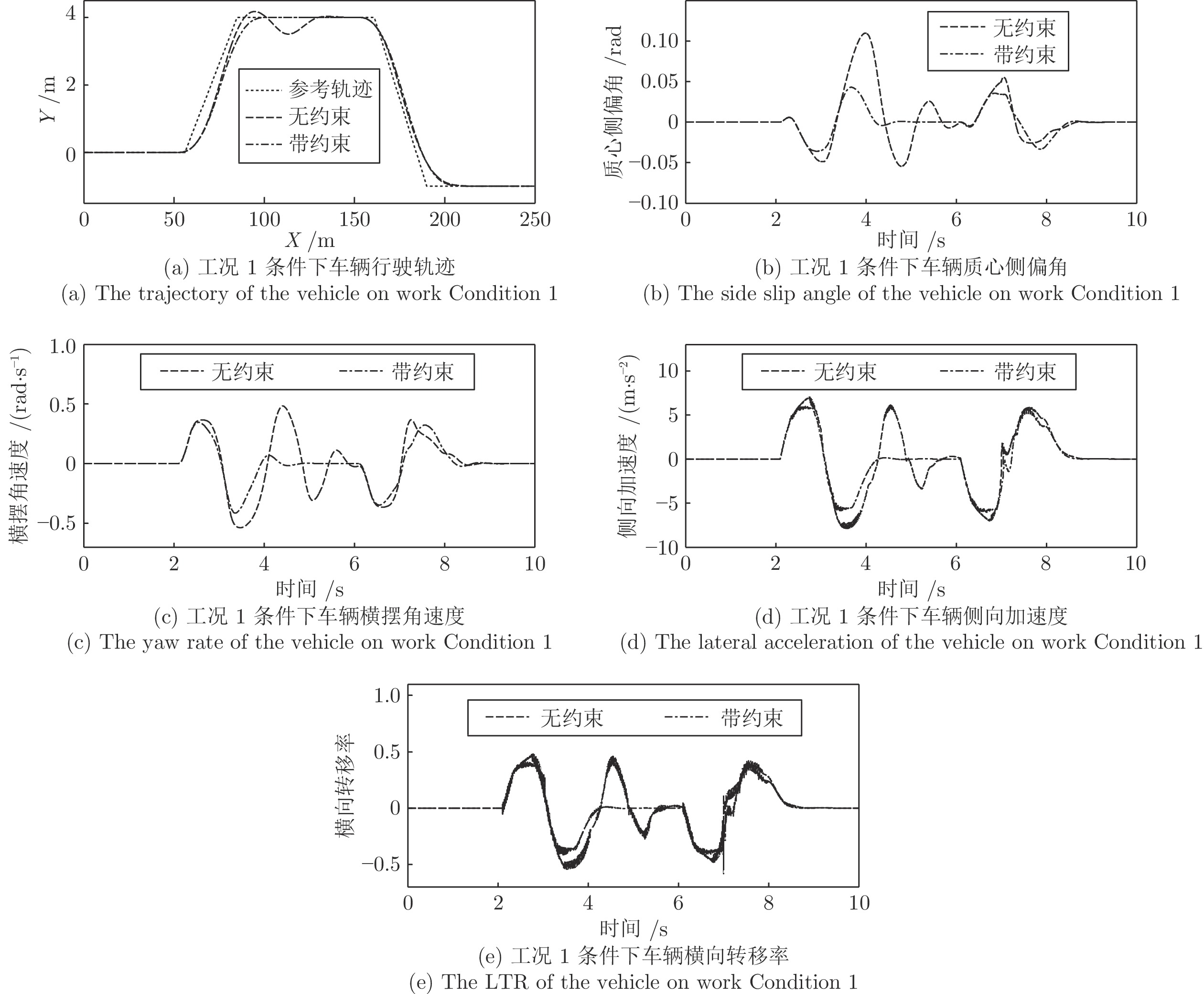
工况1. 高速双移线工况.
此工况定义车速25
${\rm{m/s}}$ , 路面附着系数为0.9, 装备不同转向控制算法的智能车辆行驶轨迹和主要系统状态如图7所示.工况2. 低路面附着系数双移线工况.
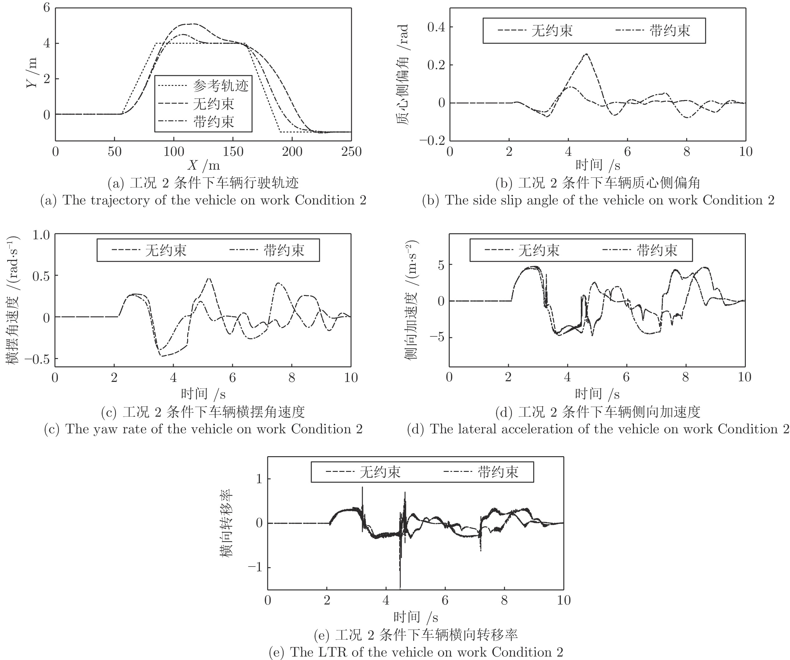
此工况定义车速25
${\rm{m/s}}$ , 路面附着系数为0.5, 装备不同转向控制算法的智能车辆行驶轨迹和主要系统状态如图8所示.工况3. 弯道路况.
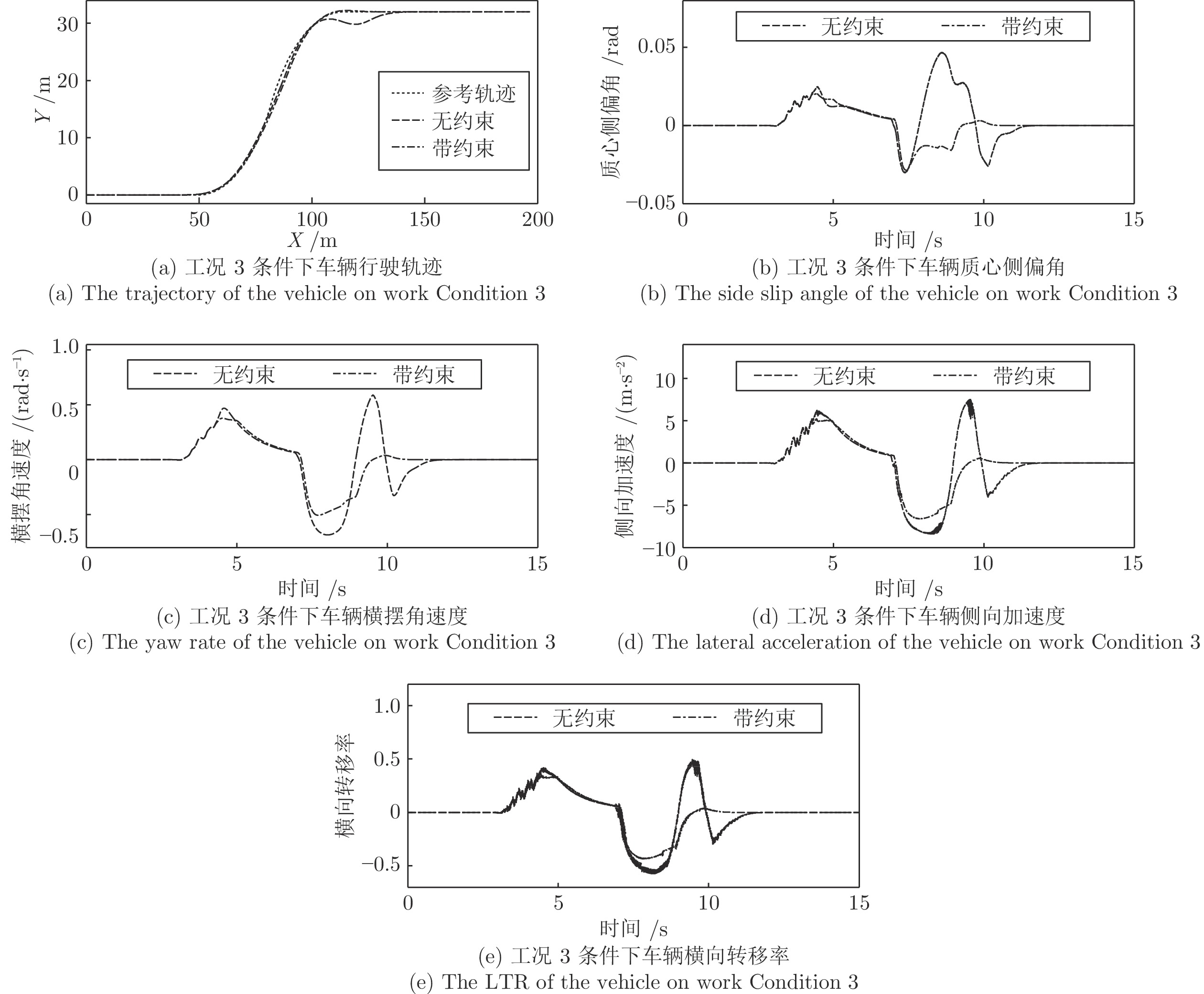
此工况下, 定义车速14
${\rm{m/s}}$ , 路面附着系数为0.9, 弯道曲率0.25. 装备不同转向控制算法的智能车辆行驶轨迹和主要系统状态如图9所示.根据实验结果, 在工况1条件下, 无约束MPC在25
${\rm{m/s}}$ 车速下轨迹跟踪的能力较差, 其在变道过程中产生了震荡. 这是因为高速行驶中车辆的侧向加速度与质心侧偏角的变化幅度大, 且不受任何约束限制, 导致车辆在行车过程中发生了失稳现象. 而带约束MPC由于质心侧偏角、横摆角速度、侧向加速度和横向转移率受弹性约束, 因此其变化幅度更小, 更加平稳, 因而其在轨迹跟踪上的效果更好.在工况2条件下, 定义车速依然保持25
${\rm{m/s}}$ 不变, 而路面附着系数减小至0.5时, 无约束MPC控制的智能车辆的轨迹跟踪效果愈发的变差, 其控制的车辆完全偏离了期望跟随的目标车道. 而车辆质心侧偏角、横摆角速度和侧向加速度也发生了大幅摆动, 稳定性变差, 而横向转移率也在某些时刻超过了1的极限值, 说明此时车辆有很严重的侧翻风险. 而带约束MPC控制的车辆尽管也偏离了原车道, 但很快恢复至正常轨迹中, 且其侧向稳定性更好.工况3的结果显示, 带约束MPC控制的车辆较好地跟随了弯道路径, 而无约束MPC控制的实验车在弯道后半程由于弯道曲率方向的改变, 其偏离了期望轨迹, 质心侧偏角、横摆角速度、侧向加速度和横向转移率的幅度加大, 其发生侧倾、侧滑等风险更高.
4.2 智能车自主换道实验验证
本节验证驾驶员模型在换道场景下的安全性、可靠性和有效性[17], 检验当前交通环境下车辆换道行驶前后的侧向轨迹、车速变化情况以及实验车与各交通车之间的安全车距. 安全车距即智能车在行驶过程中, 与环境中其他各个车辆的等效外接矩形的直线最短距离. 其效果如图10所示.
本文通过设置不同的安全间距、加速度及其增量范围和系统的反应时间来体现出智能车不一样的驾驶方式, 详细参数设置如表1所示[18].
表 1 智能驾驶员系统参数设置Table 1 The definition of the intelligent driver system实验车M Car A Car B Car C 最小安全间距${d_o}({\rm{m}})$ $ {d_o}(3) $ $ {d_o}(2) $ ${d_o}(1)$ 加速度幅度$({\rm{m/{s}}^2})$ 1.8 2.2 2.5 加速度增量$({\rm{m/{s}}^2})$ 0.09 0.11 0.12 反应时间$({\rm{s}})$ 0.4 0.7 0.9 表1中, 最小安全间距
$ {d_o} $ 由式(16)定义, 3, 2, 1是式(16)中参数$ k $ 的具体数值, 它反映了不同驾驶员对安全间距的要求. 在接下来实验中0.9为道路附着系数条件下,$ {d_o} $ 的值分别为: 5.1, 3.4和1.7.工况1. 第1种加速换道场景.
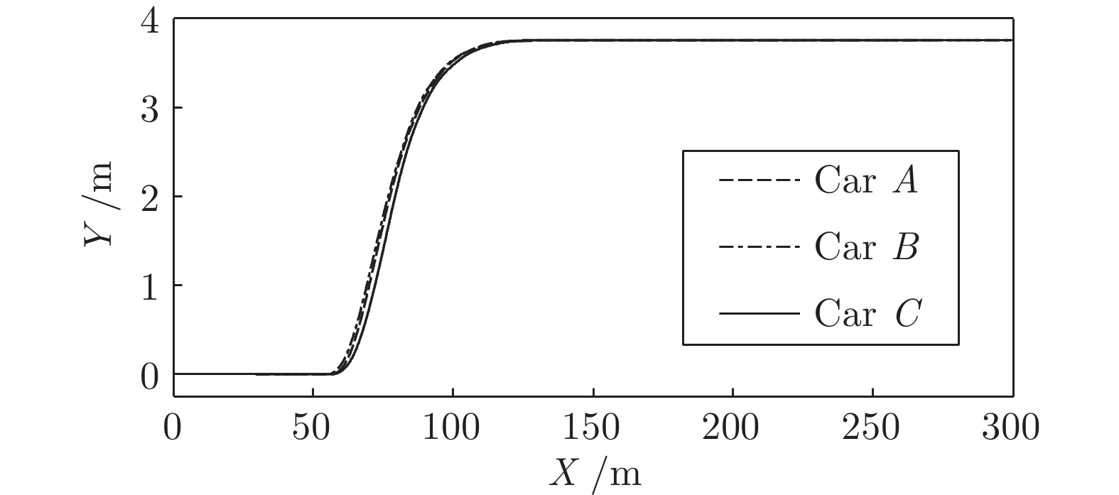
此工况下, 装备智能驾驶员模型的实验车
$ M $ 以20${\,\rm{m/s}}$ 的速度正常行驶, 此时其前方30${\,\rm{m}}$ 处交通车辆$ {L_o} $ 正以18${\,\rm{m/s}}$ 的速度匀速行驶. 其左前方车辆$ {L_o} $ 与$ M $ 初始间距5${\,\rm{m}},$ 车速25${\,\rm{m/s}}$ . 左后方车辆$F_d $ 速度20${\,\rm{m/s}}$ , 距M初始间距10${\,\rm{m}}$ . 三种智能车执行加速超车的结果如图11 ~ 15所示. 图 15 工况1智能车与目标车道后车间距Fig. 15 The distance between the intelligent vehicle with the follow vehicle of the target lane on work Condition 1
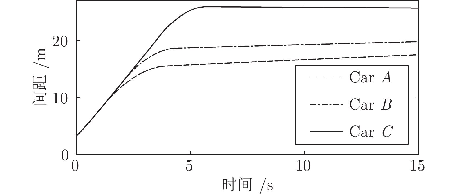 图 13 工况1智能车与原车道前车间距Fig. 13 The distance between the intelligent vehicle with the lead vehicle of the original lane on work Condition 1
 图 14 工况1智能车与目标车道前车间距Fig. 14 The distance between the intelligent vehicle with the lead vehicle of the target lane on work Condition 1
如图所示, 三种智能车均自主完成了换道行为. 车速和间距均以目标车道前车为跟车对象进行调整并逐渐趋于稳定. 从速度曲线和轨迹曲线的分析可以看出, C车因安全间距
$ {d_o} $ 比A、B两车小, 因此其启动换道的时刻最晚, 同时速度调整也越快. 根据速度曲线第45${\rm{s}}$ 时间内, C车率先减速, 目的是为保持和前车$ {L_o} $ 安全间距, 而后发现邻车道具备换道空间进而加速驶入.车间距的对比上, 各个实验车与前车
$ {L_o} $ 的最小间距一段时间内始终保持约2 m, 说明当前实验车换道后正超越前车$ {L_o} $ , 此时两车在相邻车道上并列行驶. 而换道结束后, 实验车A、B、C对车辆$ {L_d} $ 做跟车行驶并趋于稳定. 由于各车执行换道的时间不同, 三台车对$ {L_d} $ 的跟车间距有所差异. 由于A、B车同一工况下启动换道时间较早, 此时虽与$ {L_o} $ 距离较远, 但离后车$ {F_d} $ 距离较近, 最终迫使$ {F_d} $ 提前减速, 使$ {F_d} $ 与A、B车间的距离相比C车越来越大.工况2. 第2种加速换道场景
此工况下, 装备智能驾驶员模型的实验车
$ M $ 以20${\rm{m/s}}$ 的速度正常行驶, 此时其前方30${\rm{m }}$ 处交通车辆$ {L_o} $ 正以18${\rm{m/s}}$ 的速度匀速行驶. 其左前方车辆$ {L_o} $ 对$ M $ 初始间距0${\rm{m}}$ , 车速22.2${\rm{m/s}}$ . 左后方车辆速度22.2${\rm{m/s}}$ , 距M初始间距30${\rm{m}}$ . 三种智能车执行加速超车的结果如图16 ~ 20所示.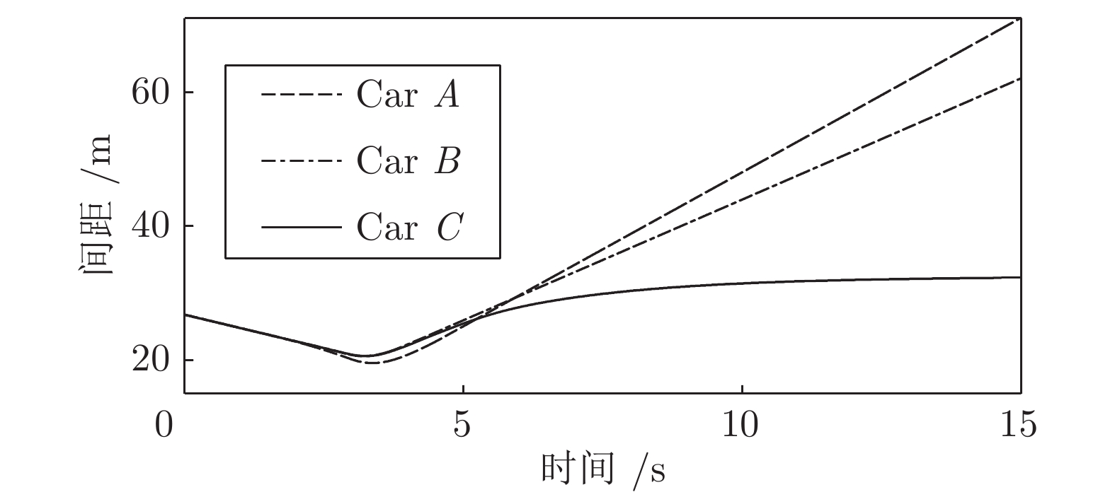 图 20 工况2智能车与目标车道后车间距Fig. 20 The distance between the intelligent vehicle with the follow vehicle of the target lane on work Condition 2
从速度曲线和轨迹曲线的分析可以看出, A车和B车由于对车辆安全间距
$ {d_o} $ 期望较高, 因此提前减速对$ {L_o} $ 进行跟车, 待与$ {L_d} $ 的间距达到期望的安全距离以后开始换道行为. C车由于对前后方的安全车距$ {d_o} $ 要求较低, 所以没有对$ {L_o} $ 跟车减速, 而是直接执行换道. 三种车在换道过程中和环境车$ {L_o}, $ $ {L_d} $ 和$ {F_d} $ 的位置关系与工况一大致相同. 且三辆车均以略小于前车$ {L_d} $ 的车速稳定行驶, 以逐步拉大与$ {L_d} $ 的间距, 保证纵向安全.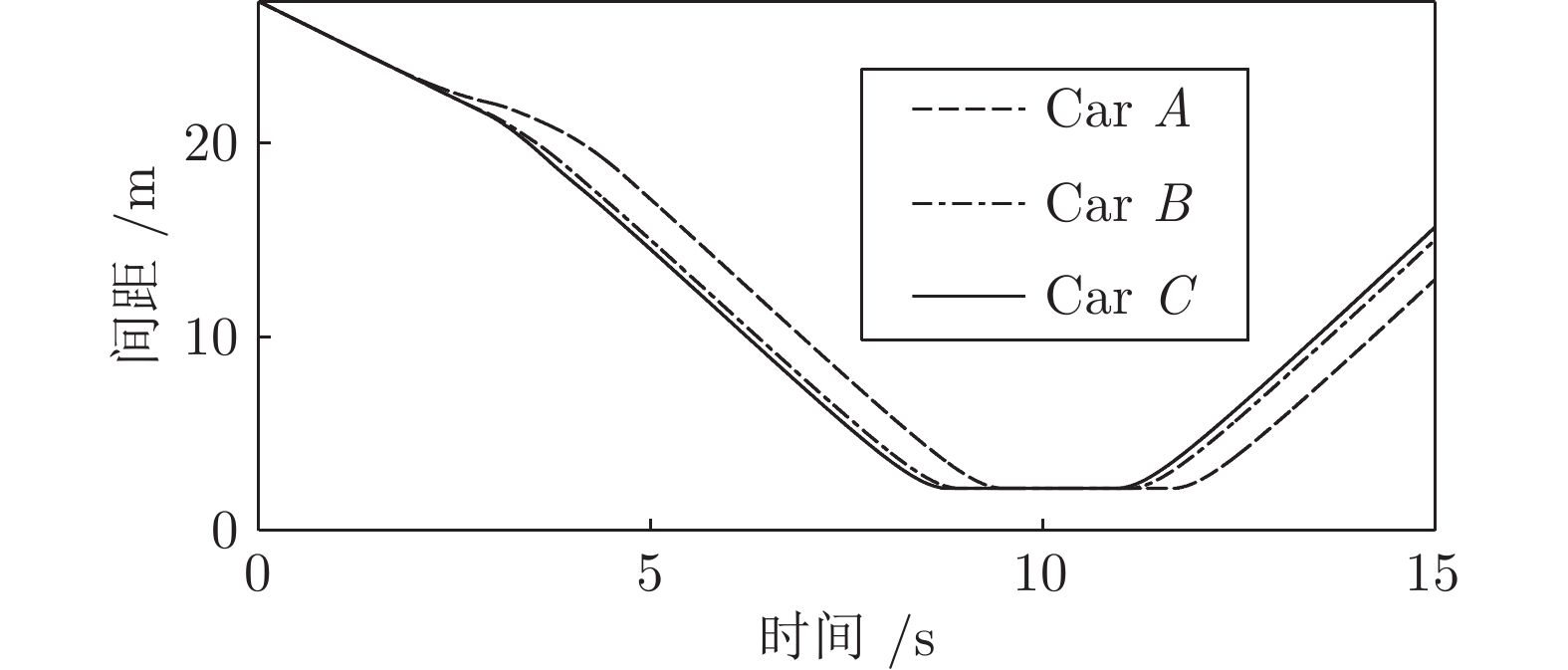 图 18 工况2智能车与原车道前车间距Fig. 18 The distance between the intelligent vehicle with the lead vehicle of the original lane on work Condition 2
 图 19 工况2智能车与目标车道前车间距Fig. 19 The distance between the intelligent vehicle with the lead vehicle of the target lane on work Condition 2
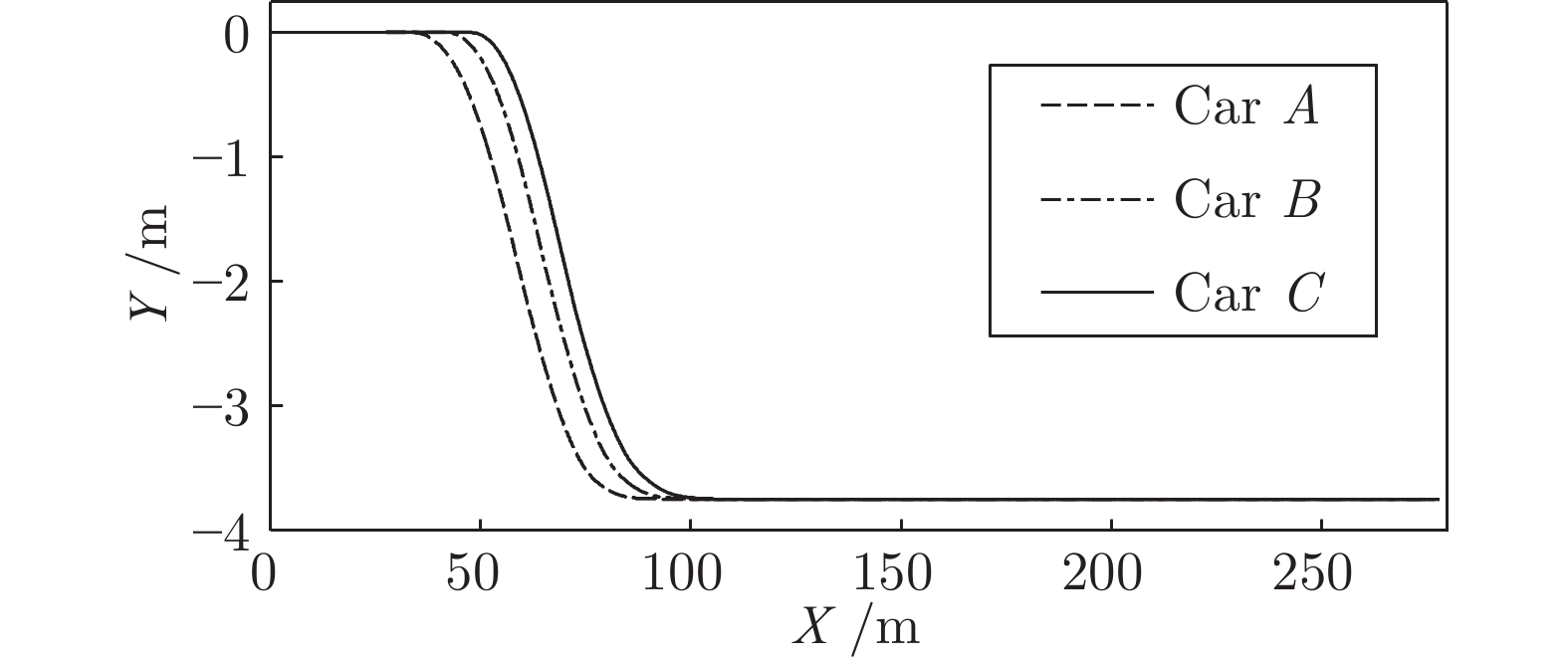
工况3. 减速换道场景
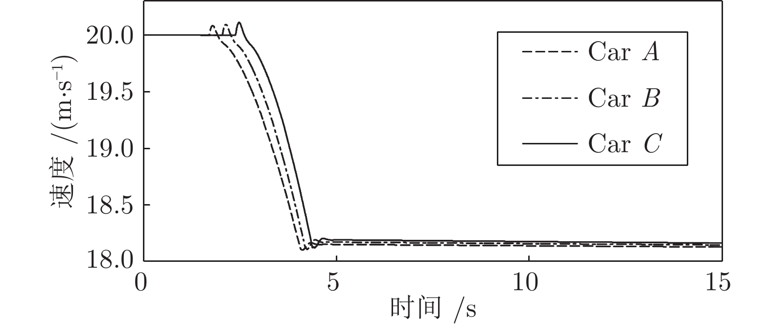
假设在工况3条件下, 装备智能驾驶员系统的实验车M以20
${\rm{m/s}}$ 的速度正常行驶, 此时其前方40${\rm{m}}$ 处交通车辆$ {L_o} $ 正以15${\rm{m/s}}$ 的速度匀速行驶. 其右前方车辆$ {L_d} $ 对M初始间距20${\rm{m}}$ , 车速18${\rm{m/s}}$ . 左后方车辆速度18${\rm{m/s}}$ , 距M初始间距10${\rm{m}}$ . 三种智能车辆执行加速超车的结果如图21 ~ 25所示.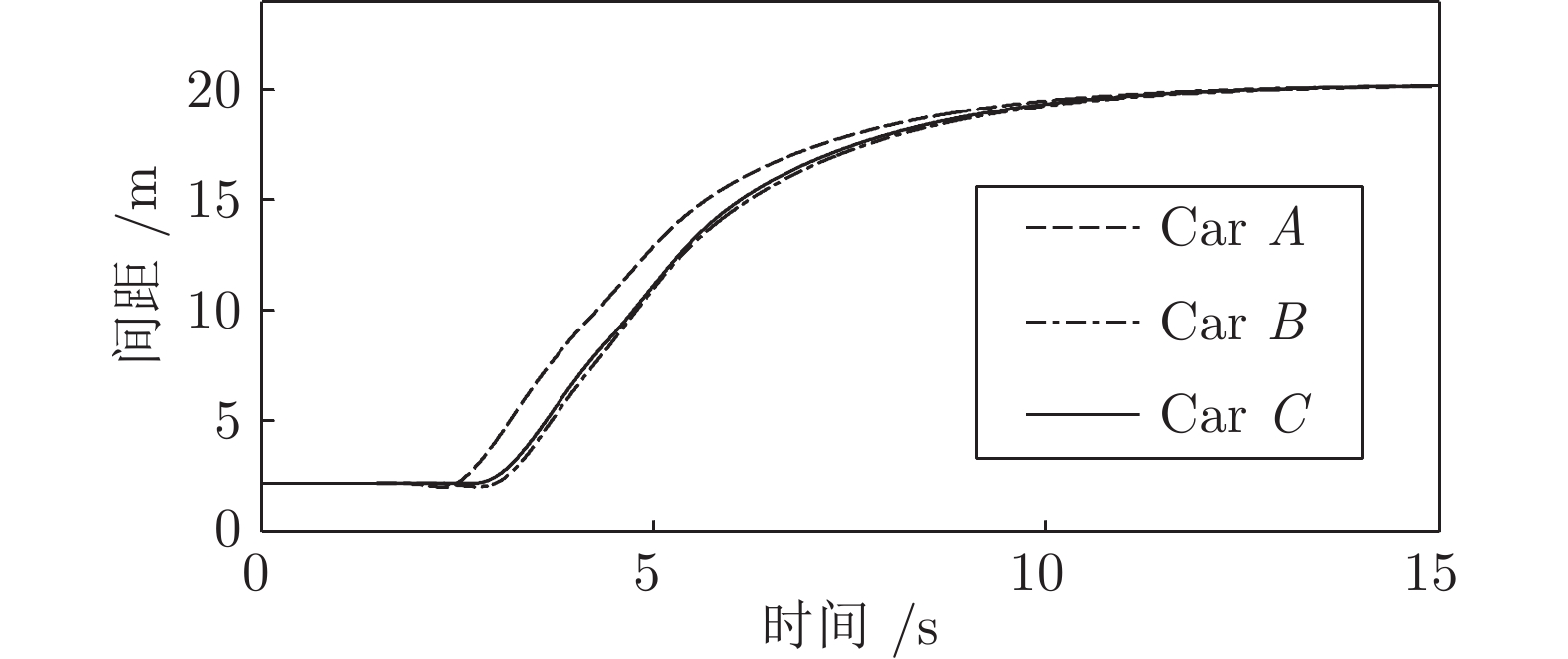 图 25 工况3智能车与目标车道后车间距Fig. 25 The distance between the intelligent vehicle with the follow vehicle of the target lane on work Condition 3
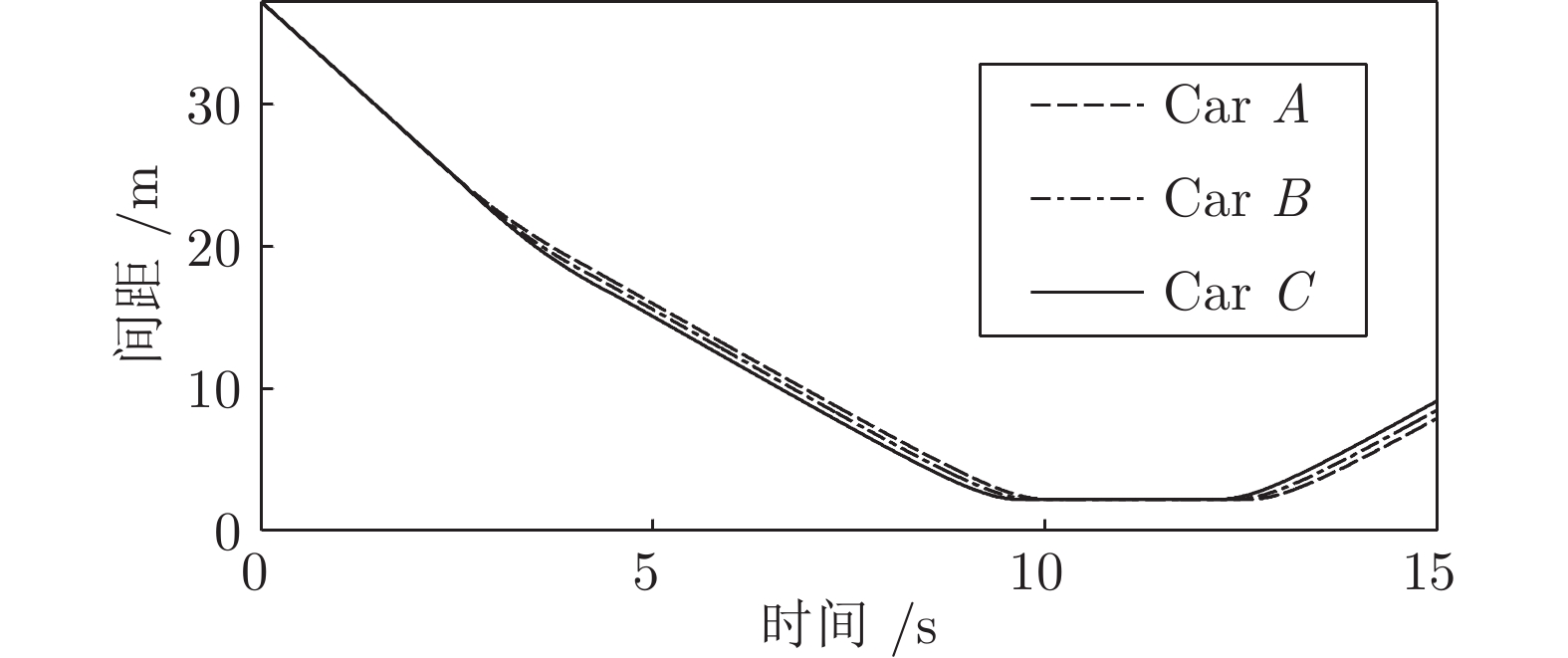 图 23 工况3智能车与原车道前车间距Fig. 23 The distance between the intelligent vehicle with the lead vehicle of the original lane on work Condition 3
 图 24 工况3智能车与目标车道前车间距Fig. 24 The distance between the intelligent vehicle with the lead vehicle of the target lane on work Condition 3
从速度曲线和轨迹曲线的分析可以看出, 由于前车
$ {L_o} $ 和目标车道的车速均小于本车车速, 且$ {L_o} $ 车速小于目标车道的前车$ {L_d} $ . 因此为了提高驾驶效率, 智能驾驶员模型选择了向车速较慢的一侧进行换道行驶. 此方案主要检验智能驾驶员模型在减速换道场景下的换道安全. 综合以上三种工况, 说明在同一种工况下, 具有不同参数的驾驶员模型往往可以体现出不同的驾驶方式.5. 结束语
本文将结合智能车在道路行驶中可能出现的安全问题, 设计了一种具有横向安全性的新型驾驶员模型. 该驾驶员模型从结构上由速度控制器、转向控制器和感知决策模块组成. 主要实现车辆准确跟踪轨迹并提高稳定性, 减小侧向安全风险, 实现自主安全换道.
首先, 转向控制器采用预测模型结合车辆质心侧偏角、横摆角速度、侧向加速度和横向转移率的约束条件相结合, 通过对性能指标与约束条件的二次规划求解, 得出车辆模型的最优控制率. 最终在高速、低路面附着系数以及转弯路况下, 转向控制器具有良好的轨迹跟踪性能和侧向稳定性.
其次, 为了避免在换道过程中与目标车道上的车辆发生碰撞, 通过对目标车道安全间距的分析, 确定出智能车执行换道的主要条件与驶入对象车道的参考加速度范围, 采用线性模型预测控制理论设计速度调整控制算法进行车速的控制. 为避免和原车道前车的发生碰撞, 采用粒子群算法计算最优的换道路径. 在三种换道工况下, 智能车均实现了通用场景下的主动换道行为, 并与环境车辆保持一定的安全间距. 不同驾驶员参数的设置, 也体现出了驾驶员模型在同一工况下的差异.
最后, 本文还存在以下改进工作:
1) 实验中设置不同驾驶员模型参数所引起的驾驶行为差异, 体现出实际行驶过程中不同驾驶员在同一路况往往体现出不一样的驾驶风格. 针对驾驶风格的定义及其判定依据和主要参数指标目前依然缺乏客观统一的依据, 后期仍需通过对真实驾驶数据的分析进行探索.
2) 实际路况复杂多样, 论文研究难以对所有复杂路况进行一一验证. 目前本文所做工作也只能在一般条件下的换道过程进行检验. 如何使智能车适应更加极端的工况以及如何建立通用的换道检验标准也将成为本文接下来要进行的工作.
-

图 6 通道交换阈值$ \theta $、正则化损失权重$ \eta $与Top-1 准确率在SUN RGB-D数据集上的关系
Fig. 6 The relationship between channel exchange threshold$ \theta $, regularization loss parameters$ \eta $, Top-1 accuracy on SUN RGB-D

图 8 通过评估不确定度动态适应模态数据质量
Fig. 8 Dynamically adapt to modal data quality by evaluating uncertainty

图 10 保留输入数据前$ k $强的属性
Fig. 10 Preserve the first$ k $strong attributes of the input data
表 1 不同模块在NYUDv2、SUN RGB-D和RGB-NIR数据集上的Top-1准确率 (%)
Table 1 Top-1 accuracies with different components on NYUDv2, SUN RGB-D and RGB-NIR (%)
树推理 树融合 通道交换 NYUDv2 SUN RGB-D RGB-NIR RGB Deep Fusion RGB Deep Fusion RGB NIR Fusion $ \times $ $ \times $ $ \times $ 43.08 59.26 71.98 52.10 38.49 62.19 58.33 52.08 77.78 $ \times $ $ \times $ √ $ 47.74^* $ $ 59.47^* $ 72.07 $ 54.29^* $ $ 47.05^* $ 66.28 $ 62.23^* $ $ 53.76^* $ 80.43 √ $ \times $ $ \times $ 46.28 57.68 72.41 50.98 36.00 58.99 58.68 53.47 79.17 √ √ $ \times $ 61.43 61.00 74.40 59.96 51.62 66.16 71.08 66.45 84.71 √ √ √ $ 71.14^* $ $ 70.99^* $ 74.74 $ 66.76^* $ $ 66.37^* $ 68.01 $ 78.85^* $ $ 77.37^* $ 85.54 注: * 表示使用通道交换为单个模态引入其他模态数据后的准确率, 加粗表示单模态或融合后最高准确率.  下载: 导出CSV
表 2 不同方法在NYUDv2、SUN RGB-D和RGB-NIR数据集上的Top-1准确率 (%)
Table 2 Top-1 accuracies with different methods on NYUDv2, SUN RGB-D and RGB-NIR (%)
方法 解释性 NYUDv2 SUN RGB-D RGB-NIR RGB Deep Fusion RGB Deep Fusion RGB NIR Fusion ViT-S-16[51] $ \times $ 54.95 62.56 — 59.23 49.43 — 74.44 66.32 — ResNet-18[49] $ \times $ 65.28 65.93 — 66.04 57.85 — 78.83 75.70 — CBCL[52] $ \times $ 56.87 63.20 73.85 50.74 43.59 65.78 74.23 62.91 81.72 TMC[19] $ \times $ 60.14 62.19 74.57 60.89 52.95 66.69 72.76 68.77 84.29 TMNR[53] $ \times $ 56.61 64.50 74.10 60.60 53.53 66.30 69.50 65.26 82.20 dNDF[54] √ 61.86 65.76 — 64.78 57.30 — 78.61 72.11 — NBDT[27] √ 65.28 62.85 — 66.20 57.93 — 74.24 74.22 — HCN[20] √ 62.20 63.18 — 61.91 53.03 — 72.92 68.75 — Ours √ $ 71.14^* $ $ 70.99^* $ 74.74 $ 66.76^* $ $ 66.37^* $ 68.01 $ 78.85^* $ $ 77.37^* $ 85.54 注: * 表示使用通道交换为单个模态引入其他模态数据后的准确率, 加粗表示单模态或融合后最高准确率.
下载: 导出CSV
表 3 不同预训练骨干网络在NYUDv2、SUN RGB-D和RGB-NIR数据集中的Top-1准确率 (%)
Table 3 Top-1 accuracies with different pretrained backbones on NYUDv2, SUN RGB-D and RGB-NIR (%)
骨干网络 NYUDv2 SUN RGB-D RGB-NIR ResNet-18 80.90 73.50 90.15 ResNet-34 81.58 73.87 90.15 ResNet-50 81.92 73.88 90.58 ResNet-101 81.93 74.96 90.79
下载: 导出CSV
表 4 插入或删除不同属性在NYUDv2、SUN RGB-D和RGB-NIR数据集中的AUC
Table 4 AUC of different attributes inserted or deleted in NYUDv2, SUN RGB-D and RGB-NIR datasets
数据集 最强属性 最弱属性 随机 插入 删除 插入 删除 插入 删除 NYUDv2 0.619 0.209 0.509 0.299 0.351 0.121 SUN RGB-D 0.601 0.300 0.463 0.380 0.284 0.168 RGB-NIR 0.636 0.380 0.549 0.466 0.355 0.207
下载: 导出CSV
-
[1] 赵静, 裴子楠, 姜斌, 陆宁云, 赵斐, 陈树峰. 基于深度强化学习的无人机虚拟管道视觉避障. 自动化学报, 2024, 50(11): 1−14Zhao Jing, Pei Zi-Nan, Jiang Bin, Lu Ning-Yun, Zhao Fei, Chen Shu-Feng. Virtual tube visual obstacle avoidance for UAV based on deep reinforcement learning. Acta Automatica Sinica, 2024, 50(11): 1−14 [2] Miikkulainen R, Liang J, Meyerson E, Rawal A, Fink D, Francon O, et al. Evolving deep neural networks. Artificial Intelligence in the Age of Neural Networks and Brain Computing (Second edition). Amsterdam: Academic Press, 2024. 269−287 [3] Hassija V, Chamola V, Mahapatra A, Singal A, Goel D, Huang K Z, et al. Interpreting black-box models: A review on explainable artificial intelligence. Cognitive Computation, 2024, 16(1): 45−74 doi: 10.1007/s12559-023-10179-8 [4] Jung J, Lee H, Jung H, Kim H. Essential properties and explanation effectiveness of explainable artificial intelligence in healthcare: A systematic review. Heliyon, 2023, 9(5): Article No. e16110 doi: 10.1016/j.heliyon.2023.e16110 [5] Costa V G, Pedreira C E. Recent advances in decision trees: An updated survey. Artificial Intelligence Review, 2023, 56(5): 4765−4800 doi: 10.1007/s10462-022-10275-5 [6] Aksjonov A, Kyrki V. A safety-critical decision-making and control framework combining machine-learning-based and rule-based algorithms. SAE International Journal of Vehicle Dynamics, Stability, and NVH, 2023, 7(3): 287−299 [7] Kitson N K, Constantinou A C, Guo Z G, Liu Y, Chobtham K. A survey of Bayesian Network structure learning. Artificial Intelligence Review, 2023, 56(8): 8721−8814 doi: 10.1007/s10462-022-10351-w [8] Simonyan K, Vedaldi A, Zisserman A. Deep inside convolutional networks: Visualising image classification models and saliency maps. In: Proceedings of the 2nd International Conference on Learning Representations (ICLR). Banff, Canada: ICLR, 2014. 1−8Simonyan K, Vedaldi A, Zisserman A. Deep inside convolutional networks: Visualising image classification models and saliency maps. In: Proceedings of the 2nd International Conference on Learning Representations (ICLR). Banff, Canada: ICLR, 2014. 1−8 [9] Sundararajan M, Taly A, Yan Q Q. Axiomatic attribution for deep networks. In: Proceedings of the 34th International Conference on Machine Learning (ICML). Sydney, Australia: JMLR, 2017. 3319−3328 [10] Zhou B L, Khosla A, Lapedriza A, Oliva A, Torralba A. Learning deep features for discriminative localization. In: Proceedings of the IEEE Conference on Computer Vision and Pattern Recognition (CVPR). Las Vegas, USA: IEEE, 2016. 2921−2929 [11] Chattopadhay A, Sarkar A, Howlader P, Balasubramanian V N. Grad-CAM++: Generalized gradient-based visual explanations for deep convolutional networks. In: Proceedings of the IEEE Winter Conference on Applications of Computer Vision (WACV). Lake Tahoe, USA: IEEE, 2018. 839−847 [12] Ribeiro M T, Singh S, Guestrin C. “Why should I trust you?”: Explaining the predictions of any classifier. In: Proceedings of the 22nd ACM SIGKDD International Conference on Knowledge Discovery and Data Mining. San Francisco, USA: Association for Computing Machinery, 2016. 1135−1144 [13] Lundberg S M, Lee S I. A unified approach to interpreting model predictions. In: Proceedings of the 31st International Conference on Neural Information Processing Systems (NIPS). Long Beach, USA: Curran Associates Inc., 2017. 4768−4777 [14] Chen C F, Li O, Tao C F, Barnett A J, Su J, Rudin C. This looks like that: Deep learning for interpretable image recognition. In: Proceedings of the 33rd International Conference on Neural Information Processing Systems (NeurIPS). Vancouver, Canada: 2019. Article No. 801Chen C F, Li O, Tao C F, Barnett A J, Su J, Rudin C. This looks like that: Deep learning for interpretable image recognition. In: Proceedings of the 33rd International Conference on Neural Information Processing Systems (NeurIPS). Vancouver, Canada: 2019. Article No. 801 [15] Nauta M, van Bree R, Seifert C. Neural prototype trees for interpretable fine-grained image recognition. In: Proceedings of the IEEE/CVF Conference on Computer Vision and Pattern Recognition (CVPR). Nashville, USA: IEEE, 2021. 14928−14938 [16] Biederman I. Recognition-by-components: A theory of human image understanding. Psychological Review, 1987, 94(2): 115−147 doi: 10.1037/0033-295X.94.2.115 [17] Cohen L G, Celnik P, Pascual-Leone A, Corwell B, Faiz L, Dambrosia J, et al. Functional relevance of cross-modal plasticity in blind humans. Nature, 1997, 389(6647): 180−183 doi: 10.1038/38278 [18] Wang Y K, Huang W B, Sun F C, Xu T Y, Rong Y, Huang J Z. Deep multimodal fusion by channel exchanging. In: Proceedings of the 34th International Conference on Neural Information Processing Systems (NeurIPS). Vancouver, Canada: Curran Associates Inc., 2020. Article No. 406 [19] Han Z B, Zhang C Q, Fu H Z, Zhou J T. Trusted multi-view classification with dynamic evidential fusion. IEEE Transactions on Pattern Analysis and Machine Intelligence, 2023, 45(2): 2551−2566 doi: 10.1109/TPAMI.2022.3171983 [20] Liu H M, Wang R P, Shan S G, Chen X L. What is a tabby? Interpretable model decisions by learning attribute-based classification criteria. IEEE Transactions on Pattern Analysis and Machine Intelligence, 2021, 43(5): 1791−1807 doi: 10.1109/TPAMI.2019.2954501 [21] Selvaraju R R, Cogswell M, Das A, Vedantam R, Parikh D, Batra D. Grad-CAM: Visual explanations from deep networks via gradient-based localization. In: Proceedings of the IEEE International Conference on Computer Vision (ICCV). Venice, Italy: IEEE, 2017. 618−626 [22] Shrikumar A, Greenside P, Kundaje A. Learning important features through propagating activation differences. In: Proceedings of the 34th International Conference on Machine Learning (ICML). Sydney, Australia: JMLR.org, 2017. 3145−3153 [23] Zeiler M D, Fergus R. Visualizing and understanding convolutional networks. In: Proceedings of the 13th European Conference on Computer Vision (ECCV). Zurich, Switzerland: Springer, 2014. 818−833 [24] Roberts L G. Machine Perception of Three-Dimensional Solids [Ph.D. dissertation], Massachusetts Institute of Technology, USA, 1963. [25] Farhadi A, Endres I, Hoiem D, Forsyth D. Describing objects by their attributes. In: Proceedings of the IEEE Conference on Computer Vision and Pattern Recognition (CVPR). Miami, USA: IEEE, 2009. 1778−1785 [26] Yang H M, Zhang X Y, Yin F, Liu C L. Robust classification with convolutional prototype learning. In: Proceedings of the IEEE/CVF Conference on Computer Vision and Pattern Recognition (CVPR). Salt Lake City, USA: IEEE, 2018. 3474−3482 [27] Wan A, Dunlap L, Ho D, Yin J H, Lee S, Petryk S, et al. NBDT: Neural-backed decision tree. In: Proceedings of the 9th International Conference on Learning Representations (ICLR). Austria: OpenReview.net, 2021.Wan A, Dunlap L, Ho D, Yin J H, Lee S, Petryk S, et al. NBDT: Neural-backed decision tree. In: Proceedings of the 9th International Conference on Learning Representations (ICLR). Austria: OpenReview.net, 2021. [28] Han X Y, Zhu X B, Pedrycz W, Li Z W. A three-way classification with fuzzy decision trees. Applied Soft Computing, 2023, 132: Article No. 109788 doi: 10.1016/j.asoc.2022.109788 [29] Islam S, Haque M M, Karim A N M R. A rule-based machine learning model for financial fraud detection. International Journal of Electrical and Computer Engineering (IJECE), 2024, 14(1): 759−771 doi: 10.11591/ijece.v14i1.pp759-771 [30] Hotelling H. Relations between two sets of variates. Breakthroughs in Statistics: Methodology and Distribution. New York: Springer, 1992. 162−190 [31] Zhang J W, Yu Y, Tang S H, Wu J M, Li W. Variational autoencoder with CCA for audio——Visual cross-modal retrieval. ACM Transactions on Multimedia Computing, Communications and Applications, 2023, 19(3s): Article No. 130 [32] Sapkota R, Thapaliya B, Suresh P, Ray B, Calhoun V D, Liu J Y. Multimodal imaging feature extraction with reference canonical correlation analysis underlying intelligence. In: Proceedings of the IEEE International Conference on Acoustics, Speech and Signal Processing (ICASSP). Seoul, Korea: IEEE, 2024. 2071−2075 [33] Tang Q, Liang J, Zhu F Q. A comparative review on multi-modal sensors fusion based on deep learning. Signal Processing, 2023, 213: Article No. 109165 doi: 10.1016/j.sigpro.2023.109165 [34] Li X J, Ma S Q, Xu J H, Tang J J, He S F, Guo F. TranSiam: Aggregating multi-modal visual features with locality for medical image segmentation. Expert Systems With Applications, 2024, 237: Article No. 121574 doi: 10.1016/j.eswa.2023.121574 [35] Zheng X, Wang M H, Huang K, Zhu E. Global and cross-modal feature aggregation for multi-omics data classification and application on drug response prediction. Information Fusion, 2024, 102: Article No. 102077 doi: 10.1016/j.inffus.2023.102077 [36] Hou M X, Zhang Z, Liu C, Lu G M. Semantic alignment network for multi-modal emotion recognition. IEEE Transactions on Circuits and Systems for Video Technology, 2023, 33(9): 5318−5329 doi: 10.1109/TCSVT.2023.3247822 [37] Song Z Y, Wei H Y, Bai L, Yang L, Jia C Y. GraphAlign: Enhancing accurate feature alignment by graph matching for multi-modal 3D object detection. In: Proceedings of the IEEE/CVF International Conference on Computer Vision (ICCV). Paris, France: IEEE, 2023. 3335−3346 [38] Xue Z H, Marculescu R. Dynamic multimodal fusion. In: Proceedings of the IEEE/CVF Conference on Computer Vision and Pattern Recognition Workshops (CVPR). Vancouver, Canada: IEEE, 2023. 2575−2584 [39] de Vries H, Strub F, Mary J, Larochelle H, Pietquin O, Courville A. Modulating early visual processing by language. In: Proceedings of the 31st International Conference on Neural Information Processing Systems (NIPS). Long Beach, USA: Curran Associates Inc., 2017. 6597−6607 [40] Du C Z, Teng J Y, Li T L, Liu Y C, Yuan T Y, Wang Y, et al. On uni-modal feature learning in supervised multi-modal learning. In: Proceedings of the 40th International Conference on Machine Learning (ICML). Honolulu, USA: JMLR.org, 2023. Article No. 345 [41] Dempster A P. Upper and lower probabilities induced by a multivalued mapping. The Annals of Mathematical Statistics, 1967, 38(2): 325−339 doi: 10.1214/aoms/1177698950 [42] Jϕsang A. Subjective Logic: A Formalism for Reasoning Under Uncertainty. Cham: Springer Publishing Company, 2016. 1−326 [43] Sensoy M, Kaplan L, Kandemir M. Evidential deep learning to quantify classification uncertainty. In: Proceedings of the 32nd International Conference on Neural Information Processing Systems (NIPS). Montréal, Canada: Curran Associates Inc., 2018. 3183−3193 [44] Higgins I, Matthey L, Pal A, Burgess C P, Glorot X, Botvinick M M, et al. Beta-VAE: Learning basic visual concepts with a constrained variational framework. In: Proceedings of the 5th International Conference on Learning Representations (ICLR). Toulon, France: OpenReview.net, 2017. [45] İrsoy O, Yildiz O T, Alpaydın E. Soft decision trees. In: Proceedings of the 21st International Conference on Pattern Recognition (ICPR). Tsukuba, Japan: IEEE, 2012. 1819−1822 [46] Silberman N, Hoiem D, Kohli P, Fergus R. Indoor segmentation and support inference from RGBD images. In: Proceedings of the 12th European Conference on Computer Vision (ECCV). Florence, Italy: Springer, 2012. 746−760 [47] Song S R, Lichtenberg S P, Xiao J X. SUN RGB-D: A RGB-D scene understanding benchmark suite. In: Proceedings of the IEEE Conference on Computer Vision and Pattern Recognition (CVPR). Boston, USA: IEEE, 2015. 567−576 [48] Brown M, Süsstrunk S. Multi-spectral SIFT for scene category recognition. In: Proceedings of the IEEE Conference on Computer Vision and Pattern Recognition (CVPR). Colorado Springs, USA: IEEE, 2011. 177−184 [49] He K M, Zhang X Y, Ren S Q, Sun J. Deep residual learning for image recognition. In: Proceedings of the IEEE Conference on Computer Vision and Pattern Recognition (CVPR). Las Vegas, USA: IEEE, 2016. 770−778 [50] Maas A L, Hannun A Y, Ng A Y. Rectifier nonlinearities improve neural network acoustic models. In: Proceedings of the 30th International Conference on Machine Learning (ICML). Atlanta, USA: JMLR, 2013. 3−8 [51] Lee S, Lee S, Song B C. Improving vision transformers to learn small-size dataset from scratch. IEEE Access, 2022, 10: 123212−123224 doi: 10.1109/ACCESS.2022.3224044 [52] Ayub A, Wagner A R. Centroid based concept learning for RGB-D indoor scene classification. In: Proceedings of the 31st British Machine Vision Conference (BMVC). Virtual Event: BMVA, 2020. 1−13Ayub A, Wagner A R. Centroid based concept learning for RGB-D indoor scene classification. In: Proceedings of the 31st British Machine Vision Conference (BMVC). Virtual Event: BMVA, 2020. 1−13 [53] Xu C, Zhang Y L, Guan Z Y, Zhao W. Trusted multi-view learning with label noise. In: Proceedings of the 33rd International Joint Conference on Artificial Intelligence (IJCAI). Jeju Island, Korea: IJCAI, 2024. 5263−5271Xu C, Zhang Y L, Guan Z Y, Zhao W. Trusted multi-view learning with label noise. In: Proceedings of the 33rd International Joint Conference on Artificial Intelligence (IJCAI). Jeju Island, Korea: IJCAI, 2024. 5263−5271 [54] Kontschieder P, Fiterau M, Criminisi A, Bulò S R. Deep neural decision forests. In: Proceedings of the IEEE International Conference on Computer Vision (ICCV). Santiago, Chile: IEEE, 2015. 1467−1475 [55] Petsiuk V, Das A, Saenko K. Rise: Randomized input sampling for explanation of black-box models. In: Proceedings of the British Machine Vision Conference (BMVC). Newcastle, UK: BMVA, 2018. 151−163 期刊类型引用(1)
1. 胡鹏,朱建新,刘昌盛,龚俊,张大庆,赵喻明. 基于状态规则的液压挖掘机虚拟驾驶员建模与仿真研究. 中南大学学报(自然科学版). 2021(04): 1118-1128 .  百度学术
百度学术其他类型引用(16)
-

 下载:
下载:


计量
- 文章访问数: 862
- HTML全文浏览量: 219
- PDF下载量: 299
- 被引次数: 17
