

Secure Control for Flexible-joint Robotic Manipulator Cyber-physical Systems Based on Fuzzy Cooperative Interaction Observer
-
摘要: 本文研究了柔性关节机械臂信息物理融合系统 (Cyber-physical systems, CPS) 在传感器测量和执行器输入受到网络攻击时的安全控制问题. 首先, 用T-S 模糊模型描述柔性关节机械臂 CPS, 描述后的模型可能存在不可测量或可测量但受传感器攻击影响的前件变量(Premise variables, PVs), 这些 PVs 直接用于构建模糊控制器会影响控制器的控制效果. 因此, 提出一类模糊协同交互观测器来构造新的、可靠的、可利用的 PVs. 同时, 该观测器能够与包含攻击估计误差(Attack estimation error, AEE)信息的辅助系统进行协同交互. 与已有结果相比, 所提出的观测器通过协同交互结构, 充分利用了 AEE 信息, 提高了攻击信号的重构精度. 在此基础上, 提出了一种具有攻击补偿结构的安全控制方案, 从而消除了传感器和执行器攻击对柔性关节机械臂CPS 性能的影响. 仿真结果验证了所提出的安全控制方案的有效性.Abstract: This paper investigates secure control problems of flexible-joint robotic manipulator cyber-physical systems (CPS) against cyber-attacks on sensor measurements and actuator inputs. Firstly, flexible-joint robotic manipulator CPS are described by the T-S fuzzy model, in which there may exist premise variables (PVs) not measured, or measured but influenced by the sensor attacks. If these PVs are directly used to construct the fuzzy controller, the control performance will be affected. Therefore, a fuzzy cooperative interaction observer is proposed to construct new, reliable and available PVs. And also the observers can cooperate with the auxiliary system which contains attack estimation error (AEE) information. Different from existing results, the proposed observer makes full use of the AEE information by the cooperative interaction structure, resulting in improvement of reconstruction accuracy of the attack signal. Furthermore, a class of secure control scheme with the attack compensation structure is given such that the influence of sensor and actuator attacks on flexible-joint robotic manipulator CPS performances is removed. The effectiveness of the proposed secure control scheme is verified by simulation results.
-
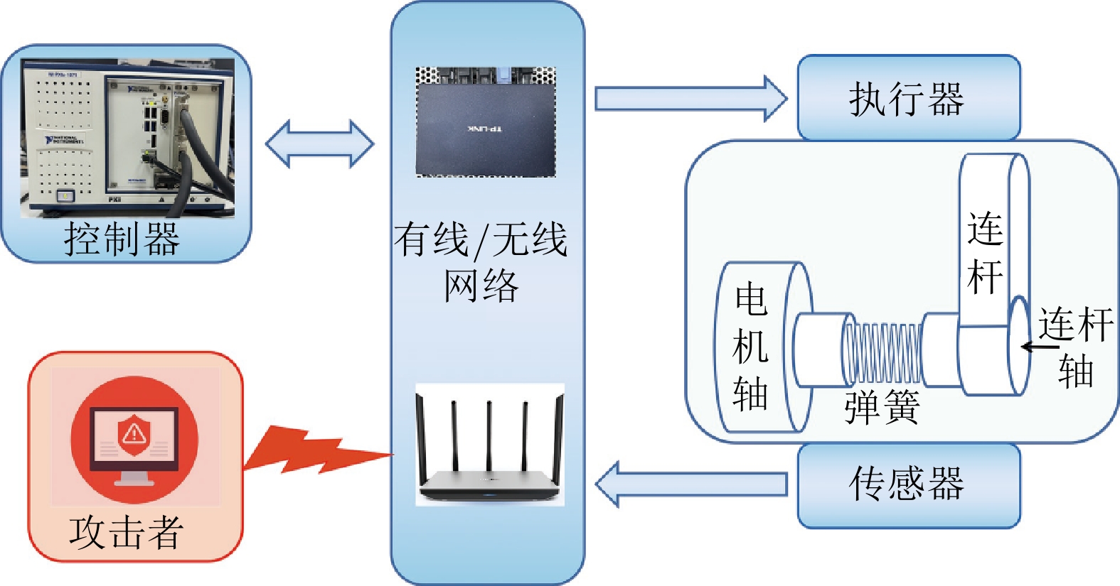
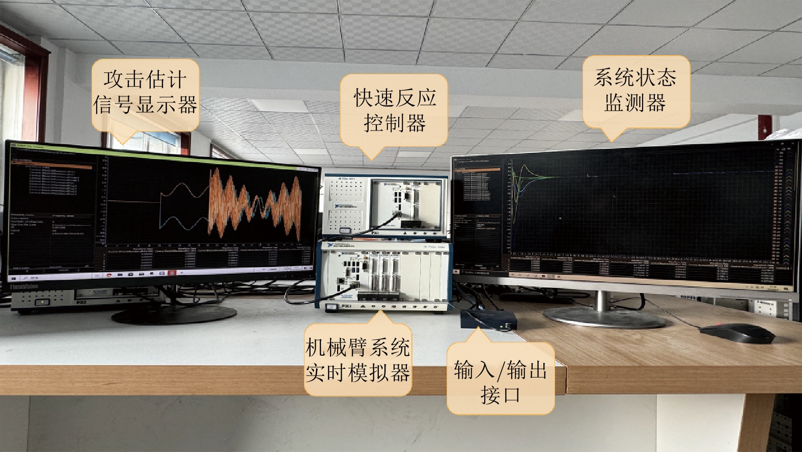
图 1 网络攻击下的单连杆柔性关节机械臂信息物理融合系统
Fig. 1 Single-link flexible-joint robotic manipulator cyber-physical systems under cyber-attacks
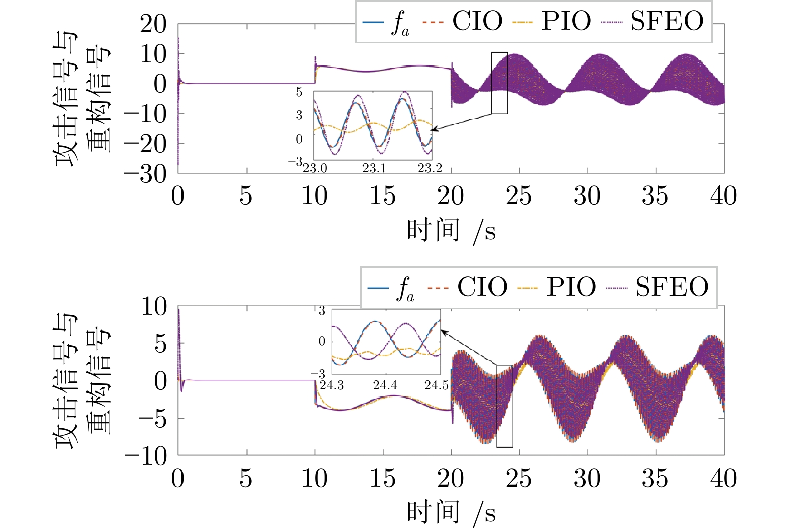
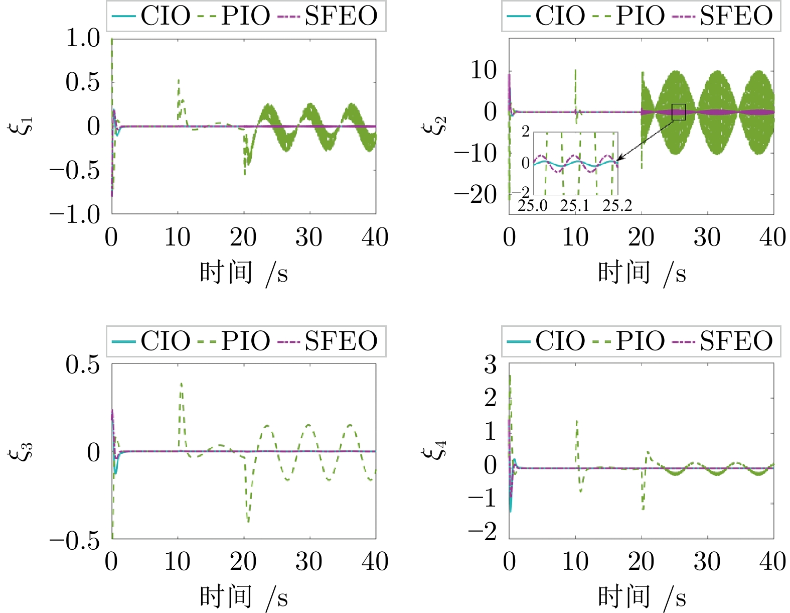
图 3 系统受到第3.1.1 节中考虑的攻击时, 在分别基于提出的 CIO, 文献[25] 的 PIO 与文献[31] 的 SFEO 的安全控制器$ U $下的系统状态响应曲线
Fig. 3 System state response curves under the security controller$U$based on the proposed CIO, the PIO in reference [25] and the SFEO in reference [31], respectively, when the system is attacked by the one considered in section 3.1.1
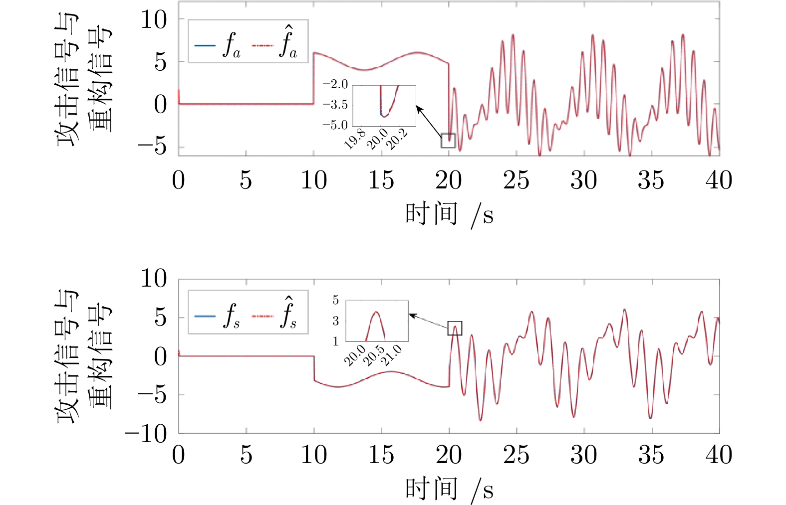
图 4 在第3.1.2 节中考虑的攻击信号与所提出观测器的重构信号的对比
Fig. 4 Comparison of the attack signals considered in section 3.1.2 with the reconstruction signals of the proposed observer
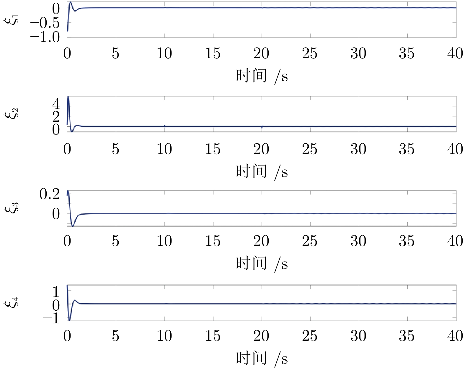
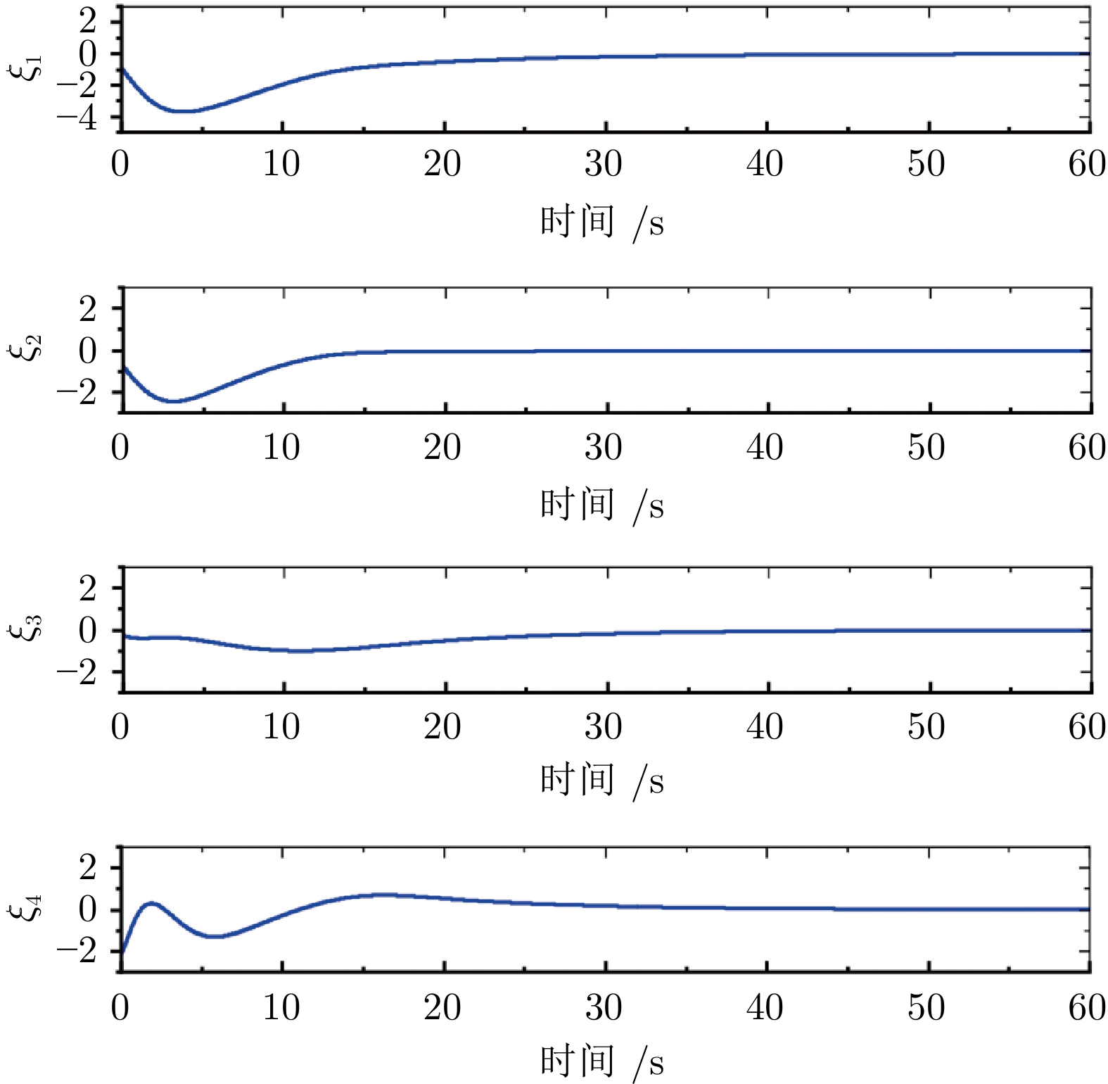
图 5 系统受到第3.1.2 节考虑的攻击时, 在基于所提出观测器的安全控制器$ U $下的系统状态响应曲线
Fig. 5 System state response curves under the security controller$U$based on the proposed observer when the system is attacked by the one considered in section 3.1.2
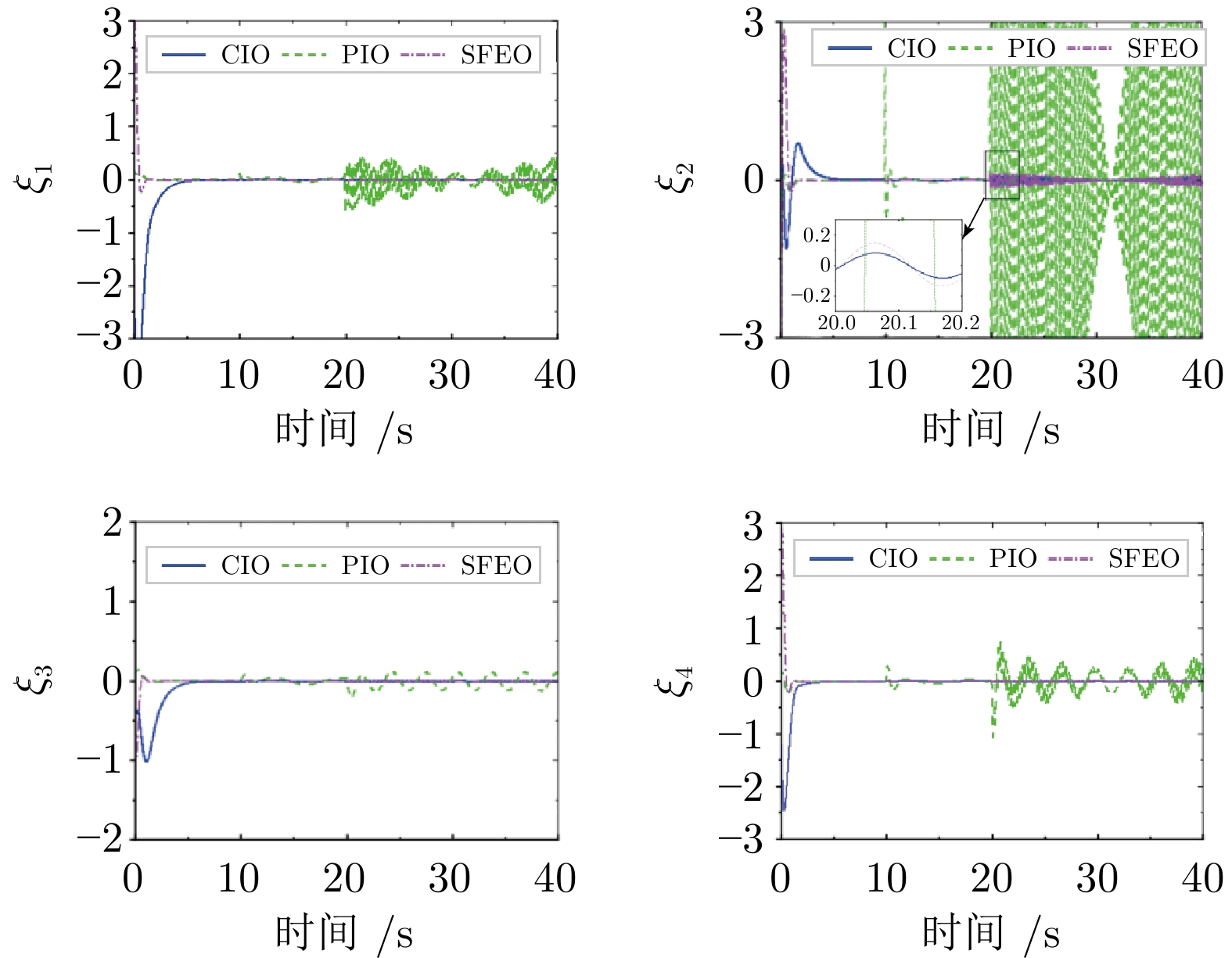
图 8 系统受到第3.2.1 节中考虑的攻击时, 在分别基于提出的 CIO, 文献[25] 的 PIO 与文献[31] 的 SFEO 的安全控制器$ U $下的系统状态响应曲线
Fig. 8 System state response curves under the security controller$U$based on the proposed CIO, the PIO in reference [25] and the SFEO in reference [31], respectively, when the system is attacked by the one considered in section 3.2.1
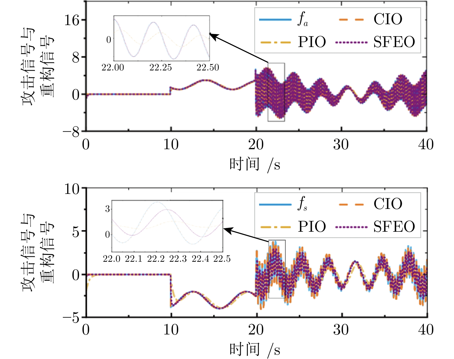
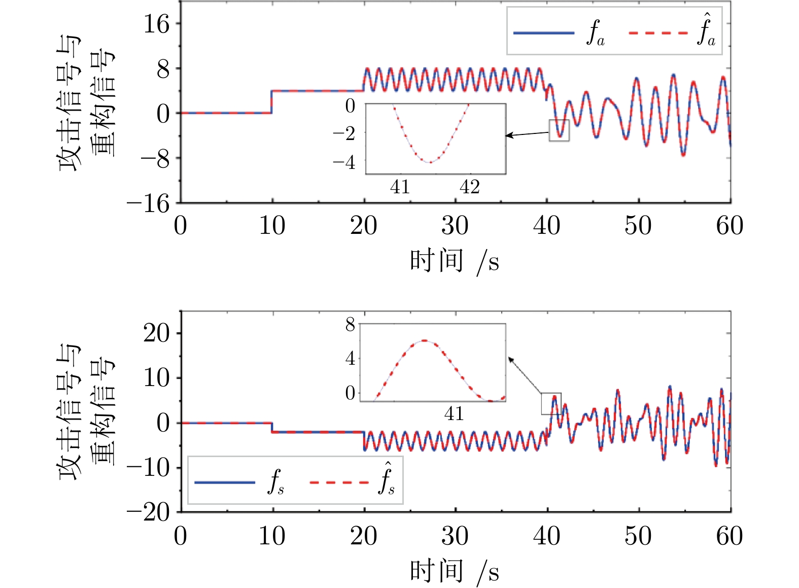
图 9 在第3.2.2 节中考虑的攻击信号与所提出观测器的重构信号的对比
Fig. 9 Comparison of the attack signals considered in section 3.2.2 with the reconstruction signals of the proposed observer
-
[1] 李洪阳, 魏慕恒, 黄洁, 邱伯华, 赵晔, 骆文城, 等. 信息物理系统技术综述. 自动化学报, 2019, 45(1): 37−50Li Hong-Yang, Wei Mu-Heng, Huang Jie, Qiu Bo-Hua, Zhao Ye, Luo Wen-Cheng, et al. Survey on cyber-physical systems. Acta Automatica Sinica, 2019, 45(1): 37−50 [2] Huang X, Li J, Su Q Y. An observer with cooperative interaction structure for biasing attack detection and secure control. IEEE Transactions on Systems, Man, and Cybernetics: Systems, 2022, 53(4): 2543−2553 [3] 原豪男, 郭戈. 交通信息物理系统中的车辆协同运行优化调度. 自动化学报, 2019, 45(1): 143−152Yuan Hao-Nan, Guo Ge. Vehicle cooperative optimization scheduling in transportation cyber physical systems. Acta Automatica Sinica, 2019, 45(1): 143−152 [4] Guo Z G, Zhang Y F, Zhao X B, Song X Y. CPS-based self-adaptive collaborative control for smart production-logistics systems. IEEE Transactions on Cybernetics, 2021, 51(1): 188−198 doi: 10.1109/TCYB.2020.2964301 [5] 杨飞生, 汪璟, 潘泉, 康沛沛. 网络攻击下信息物理融合电力系统的弹性事件触发控制. 自动化学报, 2019, 45(1): 110−119Yang Fei-Sheng, Wang Jing, Pan Quan, Kang Pei-Pei. Resilient event-triggered control of grid cyber-physical systems against cyber attack. Acta Automatica Sinica, 2019, 45(1): 110−119 [6] Ma H, Zhou Q, Li H Y, Lu R Q. Adaptive prescribed performance control of a flexible-joint robotic manipulator with dynamic uncertainties. IEEE Transactions on Cybernetics, 2022, 52(12): 12905−12915 doi: 10.1109/TCYB.2021.3091531 [7] Chang W M, Li Y M, Tong S C. Adaptive fuzzy backstepping tracking control for flexible robotic manipulator. IEEE/CAA Journal of Automatica Sinica, 2021, 8(12): 1923−1930 doi: 10.1109/JAS.2017.7510886 [8] Wang X M, Niu B, Zhao X D, Zong G D, Cheng T T, Li B. Command-filtered adaptive fuzzy finite-time tracking control algorithm for flexible robotic manipulator: A singularity-free approach. IEEE Transactions on Fuzzy Systems, DOI: 10.1109/TFUZZ.2023.3298367 [9] Yang F S, Liang X H, Guan X H. Resilient distributed economic dispatch of a cyber-power system under DoS attack. Frontiers of Information Technology & Electronic Engineering, 2021, 21(1): 40−50 [10] Li Z Q, Li Q, Ding D W, Sun X M. Robust resilient control for nonlinear systems under denial-of-service attacks. IEEE Transactions on Fuzzy Systems, 2021, 29(11): 3415−3427 doi: 10.1109/TFUZZ.2020.3022566 [11] Yan J J, Yang G H, Liu X X. A multigain-switching-mechanism-based secure estimation scheme against DoS attacks for nonlinear industrial cyber-physical systems. IEEE Transactions on Industrial Electronics, 2023, 70(5): 5094−5103 doi: 10.1109/TIE.2022.3186379 [12] Qi W H, Lv C Y, Zong G D, Ahn C K. Sliding mode control for fuzzy networked semi-markov switching models under cyber attacks. IEEE Transactions on Circuits and Systems Ⅱ: Express Briefs, 2022, 69(12): 5034−5038 doi: 10.1109/TCSII.2021.3137196 [13] Jiao S Y, Xu S Y, Park J. Hybrid-triggered-based control against denial-of-service attacks for fuzzy switched systems with persistent dwell-time. IEEE Transactions on Fuzzy Systems, DOI: 10.1109/TFUZZ.2023.3305349 [14] Liu J L, Wei L L, Xie X P, Tian E, Fei S. Quantized stabilization for T-S fuzzy systems with hybrid-triggered mechanism and stochastic cyber-attacks. IEEE Transactions on Fuzzy Systems, 2018, 26(6): 3820−3834 doi: 10.1109/TFUZZ.2018.2849702 [15] Wang X, Park J, Li H Q. Fuzzy secure event-triggered control for networked nonlinear systems under DoS and deception attacks. IEEE Transactions on Systems, Man, and Cybernetics: Systems, 2023, 53(7): 4165−4175 doi: 10.1109/TSMC.2023.3240401 [16] Gu Z, Shi P, Yue D, Yan S, Xie X P. Memory-based continuous event-triggered control for networked T-S fuzzy systems against cyberattacks. IEEE Transactions on Fuzzy Systems, 2021, 29(10): 3118−3129 doi: 10.1109/TFUZZ.2020.3012771 [17] Han C S, Lv C Y, Xie K, Qi W H, Cheng J, Shi K B, et al. Security SMC for networked fuzzy singular systems with semi-markov switching parameters. IEEE Access, 2022, 10: 45093−45101 doi: 10.1109/ACCESS.2022.3170487 [18] Li X H, Zhu F H, Chakrabarty A, Zak S. Nonfragile fault-tolerant fuzzy observer-based controller design for nonlinear systems. IEEE Transactions on Fuzzy Systems, 2016, 24(6): 1679−1689 doi: 10.1109/TFUZZ.2016.2540070 [19] 练红海, 肖伸平, 罗毅平, 周笔锋. 基于 T-S 模糊模型的采样系统鲁棒耗散控制. 自动化学报, 2022, 48(11): 2852−2862Lian Hong-Hai, Xiao Shen-Ping, Luo Yi-Ping, Zhou Bi-Feng. Robust dissipative control for sampled-data system based on T-S fuzzy model. Acta Automatica Sinica, 2022, 48(11): 2852−2862 [20] Huang X, Dong J X. An adaptive secure control scheme for T-S fuzzy systems against simultaneous stealthy sensor and actuator attacks. IEEE Transactions on Fuzzy Systems, 2021, 29(7): 1978−1991 doi: 10.1109/TFUZZ.2020.2990772 [21] Mao J, Meng X, Ding D. Fuzzy set-membership filtering for discrete-time nonlinear systems. IEEE/CAA Journal of Automatica Sinica, 2022, 9(6): 1026−1036 doi: 10.1109/JAS.2022.105416 [22] Liu Y, Wu F, Ban X J. Dynamic output feedback control for continuous-time T-S fuzzy systems using fuzzy lyapunov functions. IEEE Transactions on Fuzzy Systems, 2017, 25(5): 1155−1167 doi: 10.1109/TFUZZ.2016.2598852 [23] Zhang Z, Zhang Z X, Zhang H. Distributed attitude control for multispacecraft via Takagi-Sugeno fuzzy approach. IEEE Transactions on Aerospace and Electronic Systems, 2018, 54(2): 642−654 doi: 10.1109/TAES.2017.2761199 [24] Gao Q, Zeng X J, Feng G, Wang Y, Qiu J B. T-S-fuzzy-model-based approximation and controller design for general nonlinear systems. IEEE Transactions on Systems, Man, and Cybernetics, Part B (Cybernetics), 2012, 42(4): 1143−1154 doi: 10.1109/TSMCB.2012.2187442 [25] Mu Y F, Zhang H G, Xi R P, Wang Z L, Su J Y. Fault-tolerant control of nonlinear systems with actuator and sensor faults based on T-S fuzzy model and fuzzy observer. IEEE Transactions on Systems, Man, and Cybernetics: Systems, 2022, 52(9): 5795−5804 doi: 10.1109/TSMC.2021.3131495 [26] Tanaka K, Wang H O. Fuzzy Control Systems Design and Analysis: A Linear Matrix Inequality Approach. New York: John Wiley & Sons, 2001. [27] 王少禹, 黄开枝, 许晓明, 马克明, 陈亚军. 物理层认证的中间人导频攻击分析. 电子与信息学报, 2021, 43(11): 3141−3148 doi: 10.11999/JEIT200831Wang Shao-Yu, Huang Kai-Zhi, Xu Xiao-Ming, Ma Ke-Ming, Chen Ya-Jun. Man-in-the-middle pilot attack for physical layer authentication. Journal of Electronics & Information Technology, 2021, 43(11): 3141−3148 doi: 10.11999/JEIT200831 [28] 姚志强, 竺智荣, 叶帼华. 基于密钥协商的防范DHCP中间人攻击方案. 通信学报, 2021, 42 (8): 103−110Yao Zhi-Qiang, Zhu Zhi-Rong, Ye Guo-Hua. Achieving resist against DHCP man-in-the-middle attack scheme based on key agreement. Journal on Communications, 2021, 42 (8): 103−110 [29] Chen X L, Hu S L, Li Y, Yue D, Dou C X, Ding L. Co-estimation of state and FDI attacks and attack compensation control for multi-area load frequency control systems under FDI and DoS attacks. IEEE Transactions on Smart Grid, 2022, 13(3): 2357−2368 doi: 10.1109/TSG.2022.3147693 [30] Teixeira A, Shames I, Sandberg H, Johansson K H. A secure control framework for resource-limited adversaries. Automatica, 2015, 51: 135−148 doi: 10.1016/j.automatica.2014.10.067 [31] Ladel A, Benzaouia A, Outbib R, Ouladsine M. Integrated state/fault estimation and fault-tolerant control design for switched T-S fuzzy systems with sensor and actuator faults. IEEE Transactions on Fuzzy Systems, 2021, 30(8): 3211−3223 [32] Khalil H K. Nonlinear Systems. London: Prentice-Hall, 2002. 175−180 -

 下载:
下载:

计量
- 文章访问数: 693
- HTML全文浏览量: 228
- PDF下载量: 203
- 被引次数: 0
