

-
摘要: 在面向工业过程的计算机视觉研究中, 智能感知模型能否实际应用取决于其对复杂工业环境的适应能力. 由于可利用的工业图像数据集存在分布不均、多样性不足和干扰严重等问题, 如何生成符合多工况分布的期望训练集是提高感知模型性能的关键. 为解决上述问题, 以城市固废焚烧(Municipal solid wastes incineration, MSWI)过程为背景, 综述目前面向工业过程的图像生成及其应用研究, 为进行面向工业图像的感知建模提供支撑. 首先, 梳理面向工业过程的图像生成定义和流程以及其应用需求; 随后, 分析在工业领域中具有潜在应用价值的图像生成算法; 接着, 从工业过程图像生成、生成图像评估和应用等视角进行现状综述; 然后, 对下一步研究方向进行讨论与分析; 最后, 对全文进行总结并指出未来挑战.Abstract: In computer vision research for industrial process, the practical implementation of intelligent perception models is contingent upon their capacity for adapting to complex environments. As a result of issues such as non-uniform distribution, inadequate diversity, and significant interference within available image datasets, generating a training set that meets the multi-condition distribution is pivotal to enhance model performance. In order to address these issues, with the municipal solid wastes incineration (MSWI) process as background, this article focuses on current research on image generation and its application for industrial process, providing support for perceptual modeling for industrial images. Firstly, the definition and process of image generation for industrial process are summarized, as well as their application requirements in industrial process. Subsequently, the image generation algorithms with potential application value in the industrial domain are analyzed. Then, an overview is provided from the perspectives of industrial process image generation, generated image evaluation and application. Next, the future research direction is discussed and analyzed. Finally, we summarize the article and provide future challenges.
-

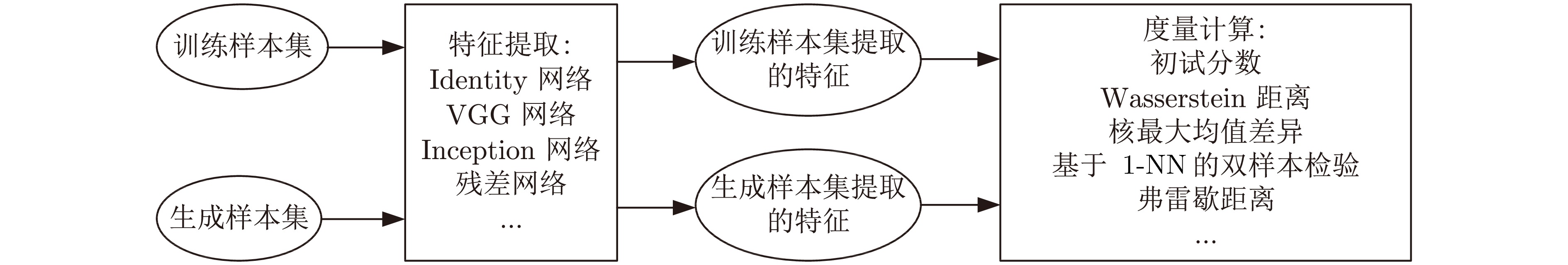
图 6 面向工业过程的图像生成及应用流程
Fig. 6 Image generation and application process for industrial process

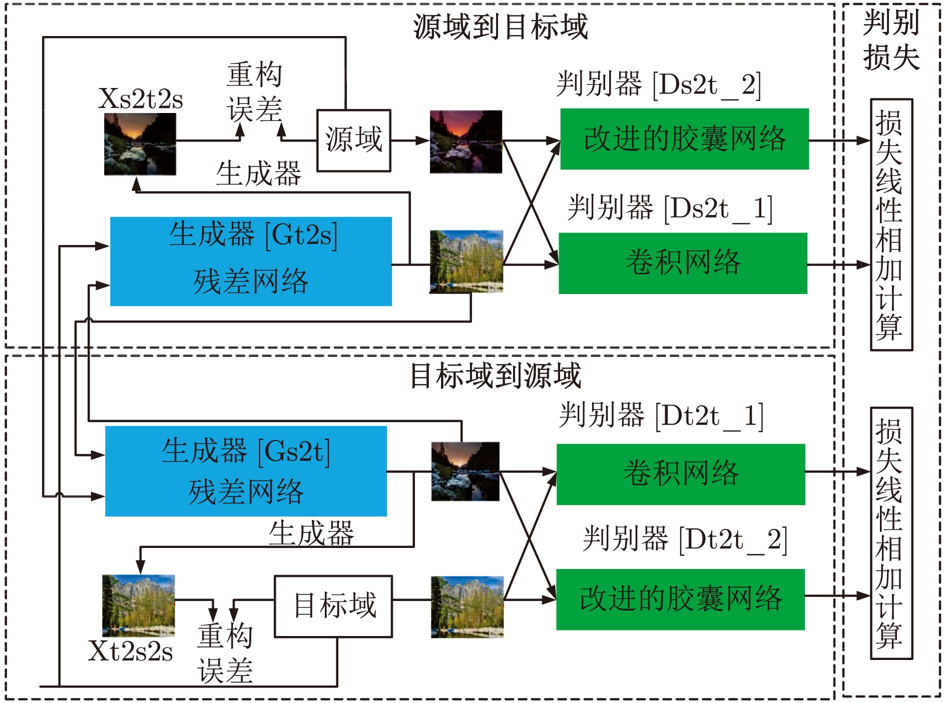
图 8 面向工业过程的图像生成及其应用研究现状结构图
Fig. 8 Structure diagram of the current research status of image generation and its application on industrial process

表 1 基于GAN的变体
Table 1 Variants based on GAN
序号 模型名称 主要贡献 文献与年份 1 cGAN 将标签信息作为附加信息输入到生成器中, 并将其与生成样本一同输入到判别器中, 进而增强生成样本与标签之间的关联性. [49], 2014 2 DCGAN 采用卷积网络作为生成器和判别器以及采用无监督的训练方法. [50], 2015 3 LAPGAN 基于拉普拉斯金字塔结构逐层增加样本分辨率, 上层高分辨率图像的生成以下层低分辨率图像作为条件. [51], 2015 4 VAE-GAN 结合VAE和GAN的混合模型. VAE用于学习输入数据的潜在空间表示, GAN中的判别器用于学习两个概率分布之间的相似度. [52], 2016 5 BiGAN 采用两个生成器和两个判别器学习训练数据的潜在表示和生成新数据. 其中, 一个生成器将随机噪声映射到数据空间, 另一个生成器将数据映射到潜在空间. 相应地, 两个判别器分别评估从潜在空间到数据空间和从数据空间到潜在空间的一对样本. [53], 2016 6 CoGAN 提出新的联合训练方法和共享权重策略, 能够同时学习多个领域之数据空间和从数据空间到潜在空间并且能够生成跨域图像.1) 联合训练: 用于同时训练多个GAN, 每个GAN对应一个领域. 通过联合训练, CoGAN可以学习多个领域之间的相关性, 并且可生成跨域图像.2) 共享权重: CoGAN的生成器和判别器之间共享权重, 可共同学习多领域间的相关性提高模型的泛化能力. 此外, CoGAN的生成器和判别器也可共享一部分权重, 进而减少模型参数的数量. [54], 2016 7 Info-GAN 引入了信息理论的概念, 使得GAN能够更有效地学习到有意义的表示和结构化的表示.1) 引入信息瓶颈: 从随机噪声向量中提取有意义的信息, 并将其与潜在变量结合生成图像, 使得GAN可对生成图像中的信息进行控制, 例如生成特定的数字或对象.2) 信息瓶颈的优化: 通过最大化互信息 (Mutual information, MI) 优化信息瓶颈. 具体地, 通过在训练过程中最大化生成数据和信息瓶颈的MI, 即目标函数是最大化生成数据与潜在编码间MI的同时最小化生成器输出与噪声间的MI, 从而实现生成图像中信息的控制. [55], 2016 8 f-GAN 证明了任意散度都适用于GAN框架. [56], 2016 9 Improved-GAN 采用多种方法对GAN的稳定性和生成效果进行进一步加强.1) 同步批量标准化 (Synchronized batch normalization, SyncBN): 将生成器和判别器的训练过程同步, 从而减少训练过程中的不稳定性, 提高训练效率和生成图像的质量.2) 动量梯度下降 (Momentum gradient descent, MGD): 采用MGD代替传统的随机梯度下降 (Stochastic gradient descent, SGD)训练生成器和判别器, 加速训练过程, 减少震荡和不稳定性.3) One-sided label smoothing: 将真实样本的标签从1降低到0.9, 减少判别器对真实样本的过度自信, 提高训练过程的稳定性和鲁棒性.4) Spectral normalization: 限制判别器中权重矩阵的最大奇异值, 减少模式崩溃的风险, 提高生成图像的多样性和质量. [57], 2016 10 WGAN-GP 将判别器的梯度作为正则项加入到判别器的损失函数中. [58], 2017 11 ACGAN 生成图像类别的控制.1) 实现生成图像类别控制: 在cGAN的基础上增加判别器以预测生成图像的类别, 在生成图像的同时学习图像的分类能力.2) 改善生成效果: 通过引入类别信息提高GAN的生成效果和多样性, 生成器和判别器相互协作使得生成的图像具有高质量以及不同的类别和特征.3) 推广应用: 不仅生成图像, 还可应用于其他数据类型, 例如声音和文本数据. [59], 2017 12 StackGAN 基于多阶段生成更高分辨率和更逼真的图像.1) 多阶段生成: 第一阶段生成低分辨率图像, 第二阶段将低分辨率图像转化为高分辨率图像, 可使得生成器更容易学习到复杂的图像结构和细节信息.2) 条件GAN结构: 将类别信息嵌入到生成器和判别器中, 能够生成指定类别的图像. 同时引入文本信息作为条件, 可根据文本描述生成图像.3) 特征金字塔 (Feature pyramid): 采用特征金字塔结构, 可同时学习不同分辨率和不同层次的图像特征, 从而生成更加逼真和细致的图像.4) 应用广泛: 可应用于不同的数据集和任务, 例如自然图像生成、文本到图像生成等. [60], 2017 13 BigGAN 实现了高分辨率图像的生成和模型的可解释性.1) 大规模模型: 最大的生成对抗网络模型之一, 具有高度可扩展性和并行性, 可生成高分辨率的真实感图像. 采用分层架构、条件归一化、投影判别器和分布式训练等技术, 可在不增加训练时间的情况下生成更高质量的图像.2) 可解释性: 提供类向量插值的图像生成方式, 可在类别之间进行平滑过渡, 生成更具艺术价值的图像. 可通过对类别和噪声向量的操纵控制生成图像的特定属性, 如颜色、纹理和形状等, 增强模型的可解释性和应用性.3) 领域拓展: 可用于各种数据类型的应用场景, 如图像生成、自然语言生成和音频合成等. [61], 2018 14 SAGAN 引入自注意力机制使得生成图像具有全局一致性和结构性.1) 自注意力机制: 在生成器和判别器中引入自注意力模块, 可在不同空间位置上学习到图像的相互依赖关系, 使生成的图像更具有全局一致性和结构性. 自注意力机制可看作是对局部区域的特征加权融合, 得到更具有语义信息的全局特征表示.2) 混合正则化: 批归一化和实例归一化相结合, 从而有效地解决生成器和判别器中的内部协变量偏移问题, 提高模型的鲁棒性和稳定性, 减少训练时间和计算成本.3) 高分辨率图像生成: 可生成更具有真实感和艺术价值的高分辨率图像, 用于许多实际场景, 例如人脸生成、自然场景生成、图像修复和视频生成等. [62], 2019 15 LSGAN 采用最小二乘损失函数, 可将图像的分布尽可能接近决策边界. [63], 2020 16 DivCo 引入对比学习, 增强条件图像生成的多样性.1) 引入对比损失: 采用对比学习以增加生成图像多样性.2) 潜在增强对比损失: 以对比的方式区分生成样本的潜在表征, 进而使得模式崩溃问题得到缓解. [64], 2021 17 Semanticspatial aware GAN 语义空间感知GAN, 通过联合训练语义分割网络和生成网络, 生成更真实、更多样且与输入条件更一致的图像.1) 引入语义信息: 通过使用语义分割网络提取输入条件的语义信息, 使生成器更好地理解输入条件.2) 对齐特征图: 通过将语义分割网络的特征图与生成器的特征图进行对齐, 使生成器更好地利用语义信息.3) 空间感知损失: 引入空间感知损失以保持生成图像与输入条件的空间一致性, 从而进一步提高生成器的性能. [65], 2022 18 RCF-GAN 提出互相对偶的特征方程GAN (Reciprocal GAN through characteristic functions, RCF-GAN), 进而能够学习到有意义的嵌入空间, 能够避免在数据域中使用均方差所产生的平滑伪影, 进而捕捉图形数据之间固有的关系. 兼具自编码器和GAN的优点, 即能够双向生成清晰图像. [66], 2023 19 WGAN 从理论上分析GAN训练不稳定的原因, 通过采用Wasserstein距离等方法提高训练稳定性. [67], 2017 20 SNGAN 基于谱归一化 (Spectral normalization, SN) 的GAN, 提高了生成器和判别器的稳定性和性能.1) SN: 采用SN技术对判别器的权重矩阵进行处理, 控制判别器范数大小, 提高稳定性和泛化能力, 减少训练过程中梯度爆炸和消失的问题, 使得训练更加稳定和快速.2) 训练技巧: 采用批次训练、增强数据和生成器先行等训练技巧, 使得生成器和判别器可以更好地学习数据分布和特征信息. 生成器先行技巧可使得生成器更容易学习到真实数据的特征, 从而生成更高质量的图像. [68], 2018 21 PGGAN 实现高分辨率图像的生成和训练过程的稳定性.1) 逐步生长: 从低分辨率图像开始训练, 逐渐增加分辨率, 增加模型的深度和复杂度, 可生成高分辨率的真实感图像和提高模型的稳定性与可训练性.2) 非线性映射: 采用非线性映射技术将噪声向量转换为高维的潜在空间向量, 增强模型的表达和生成能力, 可学习到更复杂的图像特征和结构, 生成更具艺术价值的图像.3) 归一化技术: 采用像素归一化技术, 平衡不同分辨率图像的亮度和对比度, 减少训练过程中的内部协变量偏移问题, 提高模型的可训练性和生成能力, 减少训练时间和计算成本. [69], 2018  下载: 导出CSV
表 2 基于VAE的变体
Table 2 Variants based on VAE
序号 方法名称 主要贡献 文献与年份 1 CVAE 将类别信息引入潜在空间的表示中, 能够生成特定类别的数据.1) 引入类别信息: 将条件信息作为额外输入, 并与潜在变量合并后作为一个新的潜在表示.2) 采用重参数技巧: 允许模型进行梯度反向传播, 可有效训练深度生成模型, 即将潜在变量转换为确定性变量和随机噪声的乘积.3) 最大化后验概率: 采用最大后验估计训练模型, 最大化给定输入和标签的后验概率, 可有效控制生成的数据符合特定的类别信息. [70], 2015 2 AAE 采用对抗训练的方式实现无监督学习和数据生成, 同时将潜在变量编码成固定的噪声分布, 使得数据具有可解释性.1) 无监督学习: 在无监督情况下学习数据表示, 可在不需要标签的情况下生成新数据, 对于诸多现实问题非常有效.2) 对抗训练: 采用对抗训练学习数据的表示和生成, 能够学习到数据分布的本质特征, 对于训练的稳定性有帮助.3) 潜在变量编码: 将潜在变量编码为固定的噪声分布, 而不是传统的正态分布, 能够更好地控制生成器的输出, 进而使得生成的数据更加多样化.4) 可解释性: 所学习到的数据表示具有可解释性, 其由一个编码器生成, 可通过调整潜在变量控制生成器生成的数据, 这种可解释性对图像修复、图像生成、数据增强等应用非常有价值. [71], 2015 3 IWAE 提高变分自编码器的似然下界 (Evidence lower bound, ELBO) 的上界, 能够更准确地估计后验分布.1) 提高ELBO的上界: 提出新的ELBO上界, 通过对潜在变量的重要性权重进行平均, 提高原始ELBO的上界, 使得对数似然估计更加准确.2) 更准确的后验分布估计: 通过引入具有多个重要性的采样样本, 准确地估计后验分布, 提高模型的生成能力.3) 自适应重要性采样: 选择重要性权重可更准确地估计ELBO上界和后验分布, 提高模型的生成能力.4) 基于平均的方法: 计算重要性权重, 可更准确地估计后验分布, 提高模型生成能力. [72], 2015 4 DC-IGN 可从输入图像中逆推出图像中的物体形状、位姿、材质等信息, 可用于图像编辑和重构.1) 逆图形生成: 使得模型可理解图像中的物体结构和属性.2) 图像编辑: 可采用逆推出的物体形状、位姿、材质等信息对输入图像进行编辑, 修改图像中的物体属性.3) 高效的网络结构: 采用高效的卷积神经网络结构, 可在较短的时间内学习到图像中的物体信息, 快速地生成新的图像.4) 数据集构建: 可学习到多种物体的形状、位姿、材质等信息, 可在不同的视角下观察物体, 提高模型生成能力. [73], 2015 5 LVAE 可更好地学习层次化的特征表示, 在生成样本的同时学习特征的表达方式.1) 层次化的结构: 可学习更加丰富和复杂的特征表示, 可生成更加准确和多样化的样本.2) 递归推断: 可在学习低层次特征表示的同时学习高层次特征表示, 使得模型可学习更加完整和准确的特征表示.3) 共享权重: 不同层次之间的特征表示可共享信息, 减少模型参数数量, 提高模型泛化能力. [74], 2016 6 SSVAE 新的模型结构和优化方法, 可利用有标注数据和无标注数据进行训练, 在半监督学习中性能优秀.1) 无监督和有监督的VAE结构: 无监督的VAE用于无标注数据的特征提取, 有监督的VAE用于有标注数据的特征提取.2) 优化方法: 采用SGD和重参数化技术优化无监督和有监督的VAE, 采用一个判别器优化整个模型.3) 应用于半监督学习: 性能优于其他经典的半监督学习算法, 例如半监督支持向量机 (Semi-supervised SVM)和DBN等. [75], 2017 7 infoVAE 通过最大化信息瓶颈提高VAE的信息提取能力.1) 信息瓶颈目标函数: 通过最大化信息瓶颈提高VAE的信息提取能力, 该目标函数的重构误差项用于保证模型能够还原原始数据, 互信息项用于最大化编码器和解码器之间的互信息.2) 优化方法: 采用SGD和重参数化技术优化模型, 采用额外的网络估计互信息项. [76], 2017 8 MSVAE 新的多尺度结构可同时处理不同尺度的信息, 并且能够生成高质量的图像.1) 多尺度结构: 包括一个全局编码器和多个局部编码器, 每个局部编码器对应一个尺度, 该结构可生成高质量图像.2) 融合策略: 将不同尺度的信息融合以生成最终的图像, 首先采用全局编码器生成一个潜在向量, 然后采用多个局部解码器将潜在向量解码为不同尺度的图像, 最后通过融合得到最终的图像. [77], 2017 9 RVAE 采用递归变分自编码器 (Recurrent variational autoencoders, RVAE) 学习非线性生成模型, 能够在存在异常值的情况下对数据进行建模. [78], 2018 10 CIVAE 结合自编码器s和变分自编码器的思想, 并在此基础上引入内省机制, 用于生成高质量的、多样化的、可控的图像.1) 内省机制: 帮助模型自监督和修正, 计算每个样本的重构误差和KL散度, 将这些信息用于调整模型的参数, 使模型在生成图像时更稳定和准确.2) 条件生成: 可接受额外的条件信息, 如标签或文本描述, 用于控制生成图像的特征和风格.3) 多样性: 通过引入随机噪声扰动隐含变量, 从而生成具有多种不同特征的图像. [79], 2020 11 DALL-E 基于Transformer的生成模型, 通过将文本描述编码为低维向量, 采用解码器将该向量转化为图像: 采用大规模的无监督数据集, 通过最大化ELB (Evidence lower bound) 的策略优化模型参数, 实现生成与训练数据中的不同图像. [80], 2021 12 DALL-E2 采用CLIP潜变量进行分层文本条件图像生成.1) 分层图像生成: 通过引入分层的生成过程, 将图像生成任务分解为多个子任务, 从而提高生成图像的多样性和控制能力.2) 采用CLIP模型的潜变量: 将CLIP模型生成的图像嵌入以作为潜变量, 能够捕捉到图像中的语义和风格信息, 并且可通过文本描述控制生成的图像.3) 文本条件生成: 将文本描述作为输入, 生成与描述相匹配的图像, 并可通过操纵文本描述进而生成不同层次的图像. [81], 2022 13 VPORN 1) 提出新的潜在特征增强和分布正则化框架, 用于FSL (Few-shot learning), 包括先验关系网络 (Prior relationship network, PRN) 和基于VAE的后验关系网络 (Variational posterior prediction and regularization network, VPORN). 通过PRN和VPORN, 从少量样本中学习到更多的关键类内特征和类间特征.2) 基于正则化分布估计降低标记数量不足的新颖样本的方差, 更关注关键和独特的特征, 进而避免不可控的转移. [82], 2023
下载: 导出CSV
表 3 流模型
Table 3 Flow-based model
序号 名称 主要贡献 文献与年份 1 NICE 作为首个流模型, 提出其基本框架并提出3个重要的模型结构层, 即加线耦合层、维数混合层和维数压缩层. [33], 2014 2 VINF 在VAE推断过程引入流模型结构的归一化流变分推断. [83], 2015 3 Real NVP 在耦合层中引入卷积层, 可更好地处理图像问题, 设计多尺度结构以降低模型的计算量和存储空间. [84], 2016 4 IAF 将自回归结构的流模型应用在VAE变分推断中的模型. [85], 2016 5 MAF IAF的衍生模型, 将Real NVP中的掩码卷积层引入到IAF中, 能够更好地处理图像样本, 然后提出了条件掩码自回归流CMAF, 将MAF应用到监督模型中. [86], 2017 6 GLOW 采用可逆变换将简单分布 (如高斯分布) 映射到目标分布, 从而实现高质量的样本生成和概率密度估计.1) 可逆性变换的设计和实现: 为实现高效的样本生成和概率密度估计, 采用特殊的可逆性变换, 即耦合层 (Coupling layer), 将输入数据的一部分作为输出, 另一部分通过函数变换后与输出部分进行结合, 实现了输入与输出之间的可逆性映射, 能够快速计算样本的概率密度.2) 计算图的优化和并行计算: 为加速计算和提高可扩展性, 采用计算图的优化技术, 如存储复用、内存分配和子图合并等. 此外, 采用并行计算技术以加速模型的训练和推理, 可高效地处理大规模数据集并实现快速的训练和推理.3) 在图像生成和数据压缩等领域的成功应用. [87], 2018 7 i-ResNet 以残差网络为基础的生成模型, 利用约束使残差块可逆, 用近似方法计算残差块的雅可比行列式. [88], 2019 8 ArtFlow 无偏差的图像风格转移方法.1) 无偏差的图像风格转移: 采用可逆神经流进行图像风格转移, 避免了传统方法中出现的偏差问题.2) 支持多种风格: ArtFlow可以同时支持多种风格的转移, 从而使其更加灵活. [89], 2021
下载: 导出CSV
表 5 扩散模型和Visual ChatGPT大规模模型
Table 5 Diffusion model and Visual ChatGPT large-scale model
序号 名称 主要贡献 文献与年份 1 NICS 基于梯度估计的生成建模, 其通过得分匹配估计数据分布的梯度, 利用Langevin动力学生成样本.1) 梯度估计: 当数据处于低维流形上时, 梯度未定义且难以估计, 采用不同水平的高斯噪声扰动数据并通过联合估计获得相应的得分, 即构建针对所有噪声水平扰动数据分布的梯度向量场.2) 样本生成: 采用基于退火Langevin动力学方法, 在采样过程逐渐接近数据流形时, 利用与逐渐减小的噪声水平相对应的梯度. [27], 2019 2 DDPM 引入噪声扩散模型作为生成模型, 通过迭代梯度和高斯噪声生成样本, 采用退火Langevin动力学逐渐逼近数据流形, 有效地处理低维流形上的数据生成与原始数据相似的样本. [26], 2020 3 ILVR 针对DDMP生成过程的随机性问题, 提出基于迭代潜变量细化 (Iterative latent variable refinement, ILVR)条件的方法, 在控制图像生成的同时生成高质量图像. [92], 2021 4 LDM 该潜在空间扩散模型 (Latent diffusion models, LDMs) 能够在有限的计算资源上进行扩散模型的训练, 同时保持其质量和在潜空间中训练扩散模型. 通过引入交叉注意力层, 将扩散模型转变为能够处理通用条件输入(如文本或边缘框)的强大且灵活的生成器; 通过在潜空间中进行训练能够达到细节保留与复杂度降低的平衡点, 进而实现计算需求降低和高分辨率图像合成. [93], 2021 5 ADM-G 采用UNet结构的扩散模型, 其通过增加模型的深度和宽度以使得模型的尺寸保持相对恒定; 增加了注意力机制的Heads, 采用32×32、16×16和8×8的分辨率进行注意力计算; 采用BigGAN残差模块进行上采样和下采样; 通过大量消融实验, 能够在LSUN和ImageNet 64×64的图像生成效果上达到SOTA, 打破GANs“垄断”. [94], 2022 6 Viusal ChatGPT 基于视觉基础模型, 通过对话、绘画和编辑等方式进行交互.1) 视觉基础模型: 能够处理图像输入, 通过图像与文本的联合建模进而能够更好地理解和生成与图像相关的文本.2) 多模态对话生成: 通过将视觉输入与文本对话相结合实现多模态对话的生成, 使得模型能够根据图像内容生成相关的回复.3) 绘画和编辑交互: 模型支持用户通过绘画和编辑改变生成结果, 提供了更加直观和灵活的控制方式. [95], 2023
下载: 导出CSV
表 6 工业过程图像生成问题的本质
Table 6 The essence of image generation problems in industrial process
问题描述 生成模型的表达式 下游任务采用模型的表达式 样本分布不均 ${f_{G1}}({{\boldsymbol{X}}_{{\rm{training}}}})$ ${f_{{\rm{DT1}}}}({f_{G1}}({{\boldsymbol{X}}_{{\rm{training}}}}),{{\boldsymbol{X}}_{{\rm{training}}}})$ 样本多样性不足 ${f_{G2}}({{\boldsymbol{X}}_{{\rm{training}}}},{{\boldsymbol{X}}_{{\rm{no\_label}}}})$ ${f_{{\rm{DT2}}}}({f_{G2}}({{\boldsymbol{X}}_{{\rm{training}}}},{{\boldsymbol{X}}_{{\rm{no\_label}}}}),{{\boldsymbol{X}}_{{\rm{training}}}})$ 样本噪声干扰大 ${f_{G3}}({{\boldsymbol{X}}_{{\rm{training}}}})$ ${f_{{\rm{DT3}}}}({f_{G3}}({{\boldsymbol{X}}_{{\rm{training}}}}))$
下载: 导出CSV
表 7 生成图像评估指标
Table 7 Evaluation index for generated image
方法 描述 文献与年份 1) 平均对数似然 采用从生成数据中估计的密度 (例如, 采用KDE或Parzen窗口估计)解释真实/测试数据的对数可能性, 即 [32], 2014 $L = \frac{1}{N}\sum\limits_{i = 1}^N { {\rm{log} _2} {p_{ {\rm{model} } } }} ({ {\boldsymbol{x} }_i})$ [126], 2016 2) 分类性能 评估无监督表示质量的间接技术 (例如, 特征提取、FCN得分), 可参见GAN质量指数 (GQI)[127]. [50], 2016
[110], 20173) 初试分数 (Inception score, IS) 生成数据的条件与边缘标签分布之间的KLD, 即$\exp ({{\mathop{\rm{E}}\nolimits} _{\boldsymbol{X}}}({\mathop{\rm{KL}}\nolimits} (p({\boldsymbol{y}}|{\boldsymbol{x}})||p({\boldsymbol{y}}))))$. [121], 2016 4) 判别器二样本检测 采用二分类判别器识别两个样本是否源自同一分布. [128], 2005 5) 图像质量测度 采用SSIM、PSNR和清晰度差异等指标. [129], 2004
[130], 2015
[131], 20176) 最大均值差异 从每个分布独立采样, 测量概率分布之间的差异, 如下${M_k}({p_{\rm{r} } },{p_{\rm{g} } }) = { {\rm{E} }_{ {\boldsymbol{X} },{{\boldsymbol X}' }\sim{p_{\rm{r} } } } }\left ({k({{\boldsymbol x} },{\boldsymbol{x}' })} \right) -$ $2{ {\rm{E} }_{ {\boldsymbol{X} }\sim{p_{\rm{r} } },{\boldsymbol{y} }\sim{p_{\rm{g} } } } }\left ({k({\boldsymbol{x} },{\boldsymbol{y} })} \right) + { {\rm{E} }_{ {\boldsymbol{y} },{{\boldsymbol y}' }\sim{p_{\rm{g} } } } }\left ({k({\boldsymbol{y} },{{\boldsymbol y} '})} \right)$ [132], 2012 7) 模式分数 (Mode score, MS) 与IS类似, 同时考虑标签在真实数据上的先验分布, 即$\exp ({{\mathop{\rm{E}}\nolimits} _{\boldsymbol{X}}}({\mathop{\rm{KL}}\nolimits} (p({\boldsymbol{y}}|{\boldsymbol{x}})||p({{\boldsymbol{y}}^{{\rm{train}}}}))) - {\mathop{\rm{KL}}\nolimits} (p({\boldsymbol{y}})||p({{\boldsymbol{y}}^{{\rm{train}}}}))$ [133], 2016 定量
评估8) 图像检索性能 测量图像间的最近邻距离分布:方式1. 设${\boldsymbol{d}}_{i,j}^k$是由方法$k$生成的第$j$个图像与测试图像$i$的最近邻距离, ${\boldsymbol{d}}_{i,j}^k = $ $\{ d_{1,j}^k,\cdots ,d_{n,j}^k\}$是单张图像到所有测试图像的最近邻距离的集合, 采用Wilcoxon符号秩检验假设: 两个生成器之间最接近的两个距离分布之间的差值的中值为零. 若该假设成立, 则两个生成器一样好, 否则, 其结果可用于评估哪种方法在统计上更好.方式2. 设${\boldsymbol{d}}_j^t$是第$j$个训练图像到数据集的距离, 考虑到训练集和测试集源自同一个数据集, ${\boldsymbol{d}}_j^t$可被认为是生成器达到的最优分布; 计算平均最近邻距离的相对增量以度量生成样本与理想样本间的差异, 如下式所示$\hat d_j^k = \frac{{\bar d_j^k - \bar d_j^t}}{{\bar d_j^t}},\bar d_j^k = \frac{1}{N}\sum\limits_{i = 1}^N {d_{i,j}^k} ,\bar d_j^t = \frac{1}{N}\sum\limits_{i = 1}^N {d_{i,j}^t} $ [134], 2016 9) 生成对抗度量 (Generative adversarial metric, GAM) 通过交换判别器和生成器比较两个GAN. [135], 2016 10) 覆盖率度量 生成数据覆盖真实数据的概率质量$C:= {p_{ {\rm{data} } } }(d{p_{ {\rm{model} } } } > t)$, 其中$t$使${p_{ {\rm{model} } } } (d{p_{ {\rm{model} } } } >$$t)= 0.95$. [136], 2017 11) 改进的初始分数(Modified inception score, m-IS) 侧重于从特定类别中采样图像的多样性$\exp ({ {\mathop{\rm{E} }\nolimits} _{ { {\boldsymbol{X} }_i} } }({ {\mathop{\rm{E} }\nolimits} _{ { {\boldsymbol{X} }_j} } }({\mathop{\rm{KL} }\nolimits} (p({\boldsymbol{y} }|{ {\boldsymbol{x} }_i})||p({\boldsymbol{y} }|{ {\boldsymbol{x} }_j})))))$ [137], 2017 12) 激活最大化分数(Activation maximization score, AM Score) 考虑训练标签与预测标签之间的KLD分布以及预测值的熵${\mathop{\rm{KL}}\nolimits} (p({{\boldsymbol{y}}^{{\rm{train}}}})||p({\boldsymbol{y}})) + {{\mathop{\rm{E}}\nolimits} _{\boldsymbol{X}}}(H({\boldsymbol{y}}|{\boldsymbol{x}}))$ [138], 2017 13) 弗雷歇距离 (Fréchet inception distance, FID) 多元高斯数据的特征空间数据的Wasserstein-2距离${\rm{FID}} = ||{\mu _{\rm{r}}} - {\mu _{\rm{g}}}|{|^2} +\\$ $\;\;\;\;{\rm{T} _{\rm{r}}}(Co{v_{\rm{r} } } + Co{v_{\rm{g} } } - 2{(Co{v_{\rm{r} }\times }Co{v_{\rm{g} } })^{\frac{1}{2} } })$ [122], 2017
[123], 201714) 沃瑟斯坦评判 (The Wasserstein critic) 训练神经网络, 评判真实样本为高值和低值$\hat W({ {\boldsymbol{x} }_{ {\rm{test} } } },{ {\boldsymbol{x} }_{\rm{g} } }) = \frac{1}{N}\sum\limits_{i = 1}^N {\hat f}({ {\boldsymbol{x} }_{ {\rm{test} } } }[i]) - \frac{1}{N}\sum\limits_{i = 1}^N {\hat f({ {\boldsymbol{x} }_{\rm{g} } }[i])}$ [67], 2017 15) 生日悖论测试 (Birthday paradox test) 通过计算重复数 (接近重复数) 度量离散 (连续) 分布的大小. [139], 2017 16) 对抗准确率和散度 计算两个判别器的分类精度, 一个训练于真实数据, 一个训练于生成数据, 在验证集上评估${p_{\rm{g}}}({\boldsymbol{y}}|{\boldsymbol{x}})$和${p_{\rm{r}}}({\boldsymbol{y} }|{\boldsymbol{x} })$. [140], 2017 17) 重构误差 (Reconstruction error) 通过优化$\min ||G({\boldsymbol{z}}) - {{\boldsymbol{x}}^{{\rm{test}}}}|{|^2}$测量测试图像与最近生成图像间的重构误差. [141], 2017 18) 低层次的图像统计(Low-level image statistics) 从平均功率谱、随机滤波器响应分布、对比度分布等方面评估生成图像的低层统计特征与自然场景的相似程度. [142], 2017
[143], 201719) 精确度、召回率和F1分数 用于量化GANs中的过拟合程度. [123], 2017 20) 边界失真 采用分类方法测量生成样本的多样性和协变量漂移. [144], 2018 21) 统计显著性差异(Number of statistically-different bins, NDB) 假设存在两组源自同一分布的样本集, 那么落入给定区间的样本数量在采样误差的范围内应该相等. [145], 2018 22) 比赛胜率和技能等级 设计比赛: 玩家要么是一个试图区分真实数据和虚假数据的判别器, 要么是一个试图欺骗判别器将虚假数据当作真实数据接受的生成器. [146], 2018 23) 归一化相对判别分数(Normalized relative discriminative score, NRDS) 若生成样本与真实样本更接近, 则需要更多的训练批次才能将它们与真实样本进行区分, 从而对$n$个GAN进行比较. [147], 2018 24) 几何分数 在真实数据与生成数据之间比较底层数据流形的几何属性. [148], 2018 25) 切片Wasserstein距离 (Sliced Wasserstein distance, SWD) 基于切片Wasserstein距离的生成图像评估指标. 可测量生成图像与真实图像之间的分布差异, 同时避免了FID的缺点. [69], 2018 26) 类别感知FID(Class-aware FID, CAFD) 采用高斯混合模型更好地拟合特征分布; 此外包含类别信息, 计算每个$K $类的FID并对结果求平均, 得到CAFD ${\rm{CAFD(} }{p_{\rm{r} } }{\rm{,} }{p_{\rm{g} } }{\rm{)} } = \frac{1}{K}\sum\limits_{i = 1}^K {||\mu _i^{\rm{r} } - \mu _i^{\rm{g} }||}\; +$${\rm{T}}_{\rm{r}}(Cov_i^{\rm{r}} + Cov_i^{\rm{g}} - 2{(Cov_i^{\rm{r}}\times Cov_i^{\rm{g}})^{\frac{1}{2}}})$ [149], 2018
[150], 2021定量
评估27) 无偏的FID和IS 采用外推方法来获得分数的无偏估计, 称为$\overline { {\rm{FI} }{ {\rm{D} }}}_\infty$和$\overline { {\rm{I} }{ {\rm{S} }}}_\infty$, 用无限个样本计算代替有限样本分数. [151], 2020 28) 快速FID (Fast FID) 加快FID计算的方法: 真实的样本在训练期间不会改变, 其Inception编码仅计算一次. [152], 2020 29) 空间FID (Spatial FID, SFID) FID变体, 采用空间特征取代标准的池化特征. 采用标准pool3初始特征和中间混合6/conv特征映射的前7个通道来计算FID. [153], 2021 30) 记忆感知FID (Memorization-informed FID, MiFID) FID的扩展, 除度量分布相似度, 还考虑模型对生成图像的记忆程度${\rm{MiFID}}({S_{\rm{g}}},{S_t}) = {m_\tau }({S_{\rm{g}}},{S_t})\times {s}({S_{\rm{g}}},{S_t})$其中, ${S_{\rm{g}}}$是生成数据集, ${S_t}$是真实数据集, ${m_\tau }$是基于阈值的记忆惩罚, $s({S_{\rm{g}}},{S_t})$是距离度量$s({S_{\rm{g} } },{S_t}) = \frac{1}{ {\left| { {S_{\rm{g} } } } \right|} }\sum\limits_{ {x_{\rm{g} } } \in {S_{\rm{g} } } } {\mathop {\min }\limits_{ {x_t} \in {S_t} } } (1 - \frac{ {| { < {x_{\rm{g} } }, {x_t} > } |} }{ {| { {x_{\rm{g} } } } || { {x_t} } |} })$${m_\tau }({S_{\rm{g} } },{S_t}) = \left\{ \begin{aligned} &\frac{1}{ {s({S_{\rm{g} } },{S_t})} } ,&&s({S_{\rm{g} } },{S_t})< \tau \\ &1,&&{ {\rm{otherwise} } } \end{aligned} \right.$ [154], 2021 31) 核密度估计 (Kernel density estimation, KDE) 用于估计概率密度函数形状的非参数估计方法, 通过采用核函数在数据点周围形成局部的概率密度贡献相加得到全局的概率密度函数. [155], 2022 1) 快速的场景分类 参与者被要求在很短的展示时间内 (例如100 ms) 区分生成图像和真实图像. [32], 2014 2) 近邻取样 为了检测过拟合, 生成的样本将与训练集中最近的“邻居”同时展示. 3) 网络内部结构 用于探索和说明模型的内部表征和动力学 (如空间连续性) 以及可视化学习的特征. [156], 2001
[157], 2014
[55], 2016
[158], 2016
[159], 2016
[160], 20174)偏好判断 参与者被要求根据生成图像的保真度对模型进行排名. [161], 2017
[162], 2017
[163], 2017
[164], 2018定性
评估5) 模式掉落和崩溃 对于已知模式的数据集 (例如高斯混合模型或带标签的数据集), 通过测量生成数据与模式中心的距离进行度量. [165], 2017
[166], 20176) 人眼感知评估 (Human eye perceptual evaluation, HYPE) 基于人眼视觉感知特性的图像质量评估方法. 在HYPE中, 评价者根据主观感受评估图像的质量, 评价指标通常包括多个评价者的评分, 得出图像的颜色、对比度、清晰度等, 统计质量评价结果. [167], 2019
[168], 20197) 神经得分 (Neuroscore) 采用语义分割网络比较生成图像和真实图像中分割对象的分布情况, 揭示GAN忽略某些对象类别的统计差异, 比较真实图像与GAN生成图像间的差异. [169], 2019 8) 通用的假与真检测器 (A universal fake versus real detector) 创建一个“通用”的检测器, 用于区分真实图像和生成图像, 如CNN或GAN. 在训练阶段, 该模型采用真实图像和生成图像作为输入, 以学习如何区分两类图像. 在测试阶段, 该模型对新的图像进行真假检测. [170], 2019
[171], 2020
[172], 2020
[173], 20219) 细节对比 通过细节比对检验不同GAN模型的生成效果. [174], 2022
[175], 2023
下载: 导出CSV
表 8 面向工业过程的图像生成及其应用与评估统计表
Table 8 Statistical table of image generation, application and evaluation for industrial process
子类别 方法 年份 优劣 文献 工业过程图像生成研究 样本分布
不均生成器为编码器−解码器的GAN, 引入小波对生成图像细化 2019 无缺陷区域的基本不变, 同时避免图像模糊. [102] AdaBalGAN 2019 根据分类准确性平衡每种缺陷类型的样本数量. [98] 图像处理和GAN 2019 焊接头的检测与识别. [176] 卷积编码器 (CE) 2020 基于编码的图像生成, 具有可解释性, 但多样性不足. [96] 卷积自编码器 (CAE) 2020 基于编码的图像生成, 具有可解释性, 但多样性不足. [97] EOGAN 2020 边缘特征作为先验知识指导红外图像生成. [99] 生成器是U-Net的改进GAN 2021 细化生成器的损失函数构建多传感器信息, 从而更好地增强漏磁信息. [100] 样本多样
性不足混合生成样本与实际样本训练GAN 2022 一定程度上避免模态崩溃. [101] 引入工业过程数据的GAN的图像生成 2023 创新的应用, 采用GAN来生成高炉料槽的热图; 需克服数据依赖性、模型复杂性和实际应用验证等方面的挑战. [185] SDGAN 2020 引入D2对抗损失和循环一致损失, 学习更全面的特征. [103] 采用DCGAN和CycleGAN生成缺陷图像, 采用PatchMatch和PSGAN生成无缺陷合成图像 2020 同时生成缺陷和无缺陷图像. [106] DuCaGAN 2020 在CycleGAN基础上加入胶囊网络的视觉不变性和旋转, 能够学习细节特征. [105] 缺陷区域和强度可控GAN 2021 生成缺陷的区域和强度具有可控性. [186] 具有注意力机制的循环一致性GAN (AttenCGAN) 2022 循环一致对抗网络和注意力机制解决小样本表面缺陷分类问题; 缺乏详细的实验结果和定量指标, 存在适用性的局限性以及可解释性的问题. [187] 样本噪声
干扰大pix2pix 2019 消除焊接图像中的噪声. [109] cGAN 2019 [111] PLSGAN 2021 能够增强和降噪红外热成像图像中的缺陷. [188] 工业过程生成图像应用研究 面向识别
任务基于GAN增强的缺陷识别 2019 有效提高识别模型的性能. [102] 2019 [98] 基于CAE数据增强的缺陷检测模型 2020 轻量化的深度卷积可减少模型参数和计算量, 提高缺陷检测性能. [105] 2020 [96] 2020 [97] 基于CycleGAN的周期性纹理缺陷分割框架 2017 优于现有的弱监督分割框架. [104] 基于红外图像的电气设备识别 2020 能够根据边缘特征生成图像; 采用的数据集规模相对较小, 适用性和鲁棒性有待采用更为广泛和多样化的数据集验证. [99] 管道漏磁检测 2021 集成GAN和AE, 解决标准GAN中生成的图像样本分布不均和多样性不足的问题. [100] 工业过程生成图像应用研究 面向目标
跟踪任务焊接检测 2019 结合GAN和图像处理, 建立训练样本的更新机制, 以保证模型能够覆盖所有样本. [176] 2019 采用pix2pix技术去噪, 包括图像预处理、图像选择和焊缝熔透三个阶段, 提高检测效果. [109] 具有多维信息感知和时域运动补偿的孪生网络, 进行卫星视频中的目标跟踪 2016 引入多维信息感知和时域运动补偿技术, 对于解决卫星视频中目标跟踪问题具有潜力; 缺乏实验结果的详细分析及对使用的数据集的说明. [179] 基于孪生多尺度网络的露天矿变化检测 2018 Siamese网络和多尺度信息的引入能够提高变化检测的准确性; 露天矿应用具有创新性. [181] 工业过程生成图像评估现状 定量 判别器二样本检测、图像质量测度、最大均值差异、平均对数似然、分类性能、IS、MS和FID等 (详见表7) 2005 ~ 2023 能够给出客观定量的评价指标, 具有通用性; 在面向样本多样性不足的研究中, 期望的生成样本需要服从全局分布, 而不是仅拟合训练样本的概率分布, 此类样本无法被有效评估. [32]
[110]
[122]
[123]
[126−155]定性 近邻取样网络内部结构、快速的场景分类、偏好判断、模式掉落和崩溃、HYPE、神经得分、通用的假与真检测器和细节对比 (详见表7) 2001 ~ 2023 能够观测出是否生成期望特征; 无法定量描述或给出客观指标. [32]
[156−175]
下载: 导出CSV
-
[1] Pan Y J, Yang C J, An R Q, Sun Y X. Fault detection with improved principal component pursuit method. Chemometrics and Intelligent Laboratory Systems, 2016, 157: 111-119 doi: 10.1016/j.chemolab.2016.07.003 [2] 吴高昌, 刘强, 柴天佑, 秦泗钊. 基于时序图像深度学习的电熔镁炉异常工况诊断. 自动化学报, 2019, 45(8): 1475-1485Wu Gao-Chang, Liu Qiang, Chai Tian-You, Qin Si-Zhao. Abnormal condition diagnosis through deep learning of image sequences for fused magnesium furnaces. Acta Automatica Sinica, 2019, 45(8): 1475-1485 [3] 易佞纯, 桂卫华, 梁骁俊, 张超波, 唐峰润, 阳春华. 挥发窑鼓风管的关键点识别及其摆放位置监测. 控制理论与应用, DOI: 10.7641/CTA.2023.20541Yi Ning-Chun, Gui Wei-Hua, Liang Xiao-Jun, Zhang Chao-Bo, Tang Feng-Run, Yang Chun-Hua. Keypoints identification and position monitoring of the blower pipe for volatilization kiln. Control Theory & Applications, DOI: 10.7641/CTA.2023.20541 [4] 李沛, 阳春华, 贺建军, 桂卫华. 基于影子趋势对比的矿热炉炉况在线辨识及趋势预测. 自动化学报, 2021, 47(6): 1343-1354Li Pei, Yang Chun-Hua, He Jian-Jun, Gui Wei-Hua. Smelting condition identification and prediction for submerged arc furnace based on shadow-trend-comparison. Acta Automatica Sinica, 2021, 47(6): 1343-1354 [5] Yang J C, Wang C G, Jiang B, Song H B, Meng Q G. Visual perception enabled industry intelligence: State of the art, challenges and prospects. IEEE Transactions on Industrial Informatics, 2021, 17(3): 2204-2219 doi: 10.1109/TII.2020.2998818 [6] Roy S K, Krishna G, Dubey S R, Chaudhuri B B. HybridSN: Exploring 3-D—2-D CNN feature hierarchy for hyperspectral image classification. IEEE Geoscience and Remote Sensing Letters, 2020, 17(2): 277-281 doi: 10.1109/LGRS.2019.2918719 [7] Ahammad S H, Rajesh V, Rahman M Z U, Lay-Ekuakille A. A hybrid CNN-based segmentation and boosting classifier for real time sensor spinal cord injury data. IEEE Sensors Journal, 2020, 20(17): 10092-10101 doi: 10.1109/JSEN.2020.2992879 [8] Sun Y N, Xue B, Zhang M J, Yen G G, Lv J C. Automatically designing CNN architectures using the genetic algorithm for image classification. IEEE Transactions on Cybernetics, 2020, 50(9): 3840-3854 doi: 10.1109/TCYB.2020.2983860 [9] Zhou P, Gao B H, Wang S, Chai T Y. Identification of abnormal conditions for fused magnesium melting process based on deep learning and multi-source information fusion. IEEE Transactions on Industrial Electronics, 2022, 69(3): 3017-3026 doi: 10.1109/TIE.2021.3070512 [10] Gui J, Sun Z N, Wen Y G, Tao D C, Ye J P. A review on generative adversarial networks: Algorithms, theory, and applications. IEEE Transactions on Knowledge and Data Engineering, 2023, 35(4): 3313-3332 doi: 10.1109/TKDE.2021.3130191 [11] 乔俊飞, 段滈杉, 汤健, 蒙西. 基于火焰图像特征提取的MSWI燃烧工况识别. 控制工程, 2022, 29(7): 1153-1161Qiao Jun-Fei, Duan Hao-Shan, Tang Jian, Meng Xi. Recognition of MSWI combustion conditions based on feature extraction of flame images. Control Engineering of China, 2022, 29(7): 1153-1161 [12] 汤健, 夏恒, 余文, 乔俊飞. 城市固废焚烧过程智能优化控制研究现状与展望. 自动化学报, 2023, 49(10): 2019-2059Tang Jian, Xia Heng, Yu Wen, Qiao Jun-Fei. Research status and prospects of intelligent optimization control for municipal solid waste incineration process. Acta Automatica Sinica, 2023, 49(10): 2019-2059 [13] 郭海涛, 汤健, 夏恒, 乔俊飞. 城市固废焚烧过程燃烧线极端异常火焰图像对抗生成. 中国电机工程学报, 2022Guo Hai-Tao, Tang Jian, Xia Heng, Qiao Jun-Fei. Combustion line extreme abnormal flame image adversarial generation for municipal solid waste incineration processes. Proceedings of the CSEE, 2022 [14] 郭海涛, 汤健, 丁海旭, 乔俊飞. 基于混合数据增强的MSWI过程燃烧状态识别. 自动化学报, DOI: 10.16383/j.aas.c210843Guo Hai-Tao, Tang Jian, Ding Hai-Xu, Qiao Jun-Fei. Combustion states recognition method of MSWI process based on mixed data enhancement. Acta Automatica Sinica, DOI: 10.16383/j.aas.c210843 [15] Rosenfeld A. Picture processing by computer. Computer of Monographs and Textbooks, 1969, 1(3): 147-176 [16] Salakhutdinov R. Learning deep generative models. Annual Review of Statistics & Its Application, 2015, 2(1): 361-385 [17] 刘建伟, 刘媛, 罗雄麟. 玻尔兹曼机研究进展. 计算机研究与发展, 2014, 51(1): 1-16 doi: 10.7544/issn1000-1239.2014.20121044Liu Jian-Wei, Liu Yuan, Luo Xiong-Lin. Research process of Boltzmann machine. Journal of Computer Research and Development, 2014, 51(1): 1-16 doi: 10.7544/issn1000-1239.2014.20121044 [18] 翟正利, 梁振明, 周炜, 孙霞. 变分自编码器模型综述. 计算机工程与应用, 2019, 55(3): 1-9 doi: 10.3778/j.issn.1002-8331.1810-0284Zhai Zheng-Li, Liang Zhen-Ming, Zhou Wei, Sun Xia. Research overview of variational auto-encoders models. Computer Engineering and Applications, 2019, 55(3): 1-9 doi: 10.3778/j.issn.1002-8331.1810-0284 [19] 王坤峰, 苟超, 段艳杰, 林懿伦, 郑心湖, 王飞跃. 生成式对抗网络GAN的研究进展与展望. 自动化学报, 2017, 43(3): 321-332Wang Kun-Feng, Gou Chao, Duan Yan-Jie, Lin Yi-Lun, Zheng Xin-Hu, Wang Fei-Yue. Generative adversarial networks: The state of the art and beyond. Acta Automatica Sinica, 2017, 43(3): 321-332 [20] 林懿伦, 戴星原, 李力, 王晓, 王飞跃. 人工智能研究的新前线: 生成式对抗网络. 自动化学报, 2018, 44(5): 775-792Lin Yi-Lun, Dai Xing-Yuan, Li Li, Wang Xiao, Wang Fei-Yue. The new frontier of AI research: Generative adversarial networks. Acta Automatica Sinica, 2018, 44(5): 775-792 [21] 王坤峰, 左旺孟, 谭营, 秦涛, 李力, 王飞跃. 生成式对抗网络: 从生成数据到创造智能. 自动化学报, 2018, 44(5): 769-774Wang Kun-Feng, Zuo Wang-Meng, Tan Ying, Qin Tao, Li Li, Wang Fei-Yue. Generative adversarial networks: From generating data to creating intelligence. Acta Automatica Sinica, 2018, 44(5): 769-774 [22] 胡铭菲, 左信, 刘建伟. 深度生成模型综述. 自动化学报, 2022, 48(1): 40-74Hu Ming-Fei, Zuo Xin, Liu Jian-Wei. Survey on deep generative model. Acta Automatica Sinica, 2022, 48(1): 40-74 [23] Kingma D P, Welling M. Auto-encoding variational bayes. arXiv: 1312.6114, 2022. [24] Croitoru F, Hondru V, Ionescu R T, Shah M. Diffusion models in vision: A survey. IEEE Transactions on Pattern Analysis and Machine Intelligence, 2023, 45(9): 10850-10869 doi: 10.1109/TPAMI.2023.3261988 [25] Sohl-Dickstein J, Weiss E A, Maheswaranathan N, Ganguli S. Deep unsupervised learning using nonequilibrium thermodynamics. arXiv: 1503.03585, 2015. [26] Ho J, Jain A, Abbeel P. Denoising diffusion probabilistic models. arXiv: 2006.11239, 2020. [27] Song Y, Ermon S. Generative modeling by estimating gradients of the data distribution. arXiv: 1907.05600, 2020. [28] Song Y, Sohl-Dickstein J, Kingma D P, Kumar A, Ermon S, Poole B. Score-based generative modeling through stochastic differential equations. arXiv: 2011.13456, 2021. [29] Smolensky P. Parallel Distributed Processing: Explorations in the Microstructure of Cognition. Cambridge: MIT Press, 1987. 194−281 [30] Hinton G E, Osindero S, Teh Y. A fast learning algorithm for deep belief nets. Neural Compuper, 2006, 18(7): 1527-1554 doi: 10.1162/neco.2006.18.7.1527 [31] Salakhutdinov R, Hinton G E. Deep Boltzmann machines. In: Proceedings of the International Conference on Artificial Intelligence and Statistics. Shanghai, China: PMLR, 2009. 448−455 [32] Goodfellow I J, Pouget-Abadie J, Mirza M, Xu B, Warde-Farley D, Ozair S, et al. Generative adversarial nets. In: Proceedings of the 27th International Conference on Neural Information Processing Systems. Montreal, Canada: MIT Press, 2014. 2672−2680 [33] Dinh L, Krueger D, Bengio Y. NICE: Non-linear independent components estimation. arXiv: 1410.8516, 2015. [34] Larochelle H, Murray I. The neural autoregressive distribution estimator. In: Proceedings of the Fourteenth International Conference on Artificial Intelligence and Statistics. Fort Lauderdale, USA: PMLR, 2011. 29−37 [35] Oord A V D, Kalchbrenner N, Kavukcuoglu K. Pixel recurrent neural networks. arXiv: 1601.06759, 2016. [36] Germain M, Gregor K, Murray I, Larochelle H. MADE: Masked autoencoder for distribution estimation. In: Proceedings of the 32nd International Conference on International Conference on Machine Learning. Lille, France: JMLR, 2015. 881−889 [37] Socher R, Pennington J, Huang E H, Ng A Y, Manning C D. Semi-supervised recursive autoencoders for predicting sentiment distributions. In: Proceedings of the Conference on Empirical Methods in Natural Language Processing. Edinburgh, UK: Association for Computational Linguistics, 2011. 151−161 [38] Xu Q T, Huang G, Yuan Y, Guo C, Sun Y, Wu F, et al. An empirical study on evaluation metrics of generative adversarial networks. arXiv: 1806.07755, 2018. [39] Duan J J, He Y G, Du B L, Ghandour R M R, Wu W J, Zhang H. Intelligent localization of transformer internal degradations combining deep convolutional neural networks and image segmentation. IEEE Access, 2019, 7: 62705-62720 doi: 10.1109/ACCESS.2019.2916461 [40] Gong X J, Yao Q, Wang M L, Lin Y. A deep learning approach for oriented electrical equipment detection in thermal images. IEEE Access, 2018, 6: 41590-41597 doi: 10.1109/ACCESS.2018.2859048 [41] Zhao Z B, Fan X Q, Xu G Z, Zhang L, Qi Y C, Zhang K. Aggregating deep convolutional feature maps for insulator detection in infrared images. IEEE Access, 2017, 5: 21831-21839 doi: 10.1109/ACCESS.2017.2757030 [42] Jia F, Lei Y G, Lu N, Xing S B. Deep normalized convolutional neural network for imbalanced fault classication of machinery and its understanding via visualization. Mechanical Systems and Signal Processing, 2018, 110: 349-367 doi: 10.1016/j.ymssp.2018.03.025 [43] Gadermayr M, Li K, Müller M, Truhn D, Krämer N, Merhof D, et al. Domain-specic data augmentation for segmenting MR imagesof fatty infiltrated human thighs with neural networks. Journal of Magnetic Resonance Imaging, 2019, 49(6): 1676-1683 doi: 10.1002/jmri.26544 [44] Zhu X Y, Liu Y F, Qin Z C, Li J H. Data augmentation in emotion classification using generative adversarial networks. arXiv: 1711.00648, 2017. [45] He K M, Zhang X Y, Ren S Q, Sun J. Deep residual learning for image recognition. In: Proceedings of the IEEE Conference on Computer Vision and Pattern Recognition (CVPR). Las Vegas, USA: IEEE, 2016. 770−778 [46] Gao X, Deng F, Yue X H. Data augmentation in fault diagnosis based on the Wasserstein generative adversarial network with gradient penalty. Neurocomputing, 2020, 396: 487-494 doi: 10.1016/j.neucom.2018.10.109 [47] Wong S C, Gatt A, Stamatescu V, McDonnell M D. Understanding data augmentation for classication: When to warp? In: Proceedings of the International Conference on Digital Image Computing: Techniques and Applications (DICTA). Gold Coast, Australia: IEEE, 2016. 1−6 [48] Cuello K C, Chacón M, Mery D, Acuña G. Neural network method for failure detection with skewed class distribution. Insight, 2004, 46(7): 399-402 doi: 10.1784/insi.46.7.399.55578 [49] Mirza M, Osindero S. Conditional generative adversarial nets. arXiv: 1411.1784, 2014. [50] Radford A, Metz L, Chintala S. Unsupervised representation learning with deep convolutional generative adversarial networks. arXiv: 1511.06434, 2016. [51] Denton E, Chintala S, Szlam A, Fergus R. Deep generative image models using a Laplacian pyramid of adversarial networks. arXiv: 1506.05751, 2015. [52] Larsen A B L, Sonderby S K, Larochelle H, Winther O. Autoencoding beyond pixels using a learned similarity metric. In: Proceedings of the 33rd International Conference on International Conference on Machine Learning. New York, USA: JMLR, 2016. 1558−1566 [53] Donahue J, Krahenbühl P, Darrell T. Adversarial feature learning. arXiv: 1605.09782, 2017. [54] Liu M Y, Tuzel O. Coupled generative adversarial networks. In: Proceedings of the 30th International Conference on Neural Information Processing Systems. New York, USA: Curran Associates Inc., 2016. 469−477 [55] Chen X, Duan Y, Houthooft R, Schulman J, Sutskever I, Abbeel P. InfoGAN: Interpretable representation learning by information maximizing generative adversarial nets. In: Proceedings of the 30th International Conference on Neural Information Processing Systems. Barcelona, Spain: Curran Associates Inc., 2016. 2180−2188 [56] Nowozin S, Cseke B, Tomioka R. f-GAN: Training generative neural samplers using variational divergence minimization. In: Proceedings of the 30th International Conference on Neural Information Processing Systems. Barcelona, Spain: Curran Associates Inc., 2016. 271−279 [57] Salimans T, Goodfellow I, Zaremba W, Cheung V, Radford A, Chen X. Improved techniques for training GANs. In: Proceedings of the 30th International Conference on Neural Information Processing Systems. Barcelona, Spain: Curran Associates Inc., 2016. 2234−2232 [58] Gulrajani I, Ahmed F, Arjovsky M, Dumoulin V, Courville A C. Improved training of wasserstein GANs. In: Proceedings of the 31st International Conference on Neural Information Processing Systems. Long Beach, USA: Curran Associates Inc., 2017. 5769−5779 [59] Odena A, Olah C, Shlens J. Conditional image synthesis with auxiliary classifier GANs. In: Proceedings of the 34th International Conference on Machine Learning. Sydney, Australia: JMLR, 2017. 2642−2651 [60] Zhang H, Xu T, Li H S, Zhang S T, Wang X G, Huang X L, et al. StackGAN: Text to photo-realistic image synthesis with stacked generative adversarial networks. In: Proceedings of the IEEE International Conference on Computer Vision (ICCV). Venice, Italy: IEEE, 2017. 5908−5916 [61] Brock A, Donahue J, Simonyan K. Large scale GAN training for high fidelity natural image synthesis. arXiv: 1809.11096, 2019. [62] Zhang H, Goodfellow I, Metaxas D, Odena A. Self-attention generative adversarial networks. arXiv: 1805.08318, 2019. [63] Qi G J. Loss-sensitive generative adversarial networks on Lipschitz densities. International Journal of Computer Vision, 2020, 128(5): 1118-1140 doi: 10.1007/s11263-019-01265-2 [64] Liu R, Ge Y X, Choi C L, Wang X G, Li H S. DivCo: Diverse conditional image synthesis via contrastive generative adversarial network. In: Proceedings of the IEEE/CVF Conference on Computer Vision and Pattern Recognition (CVPR). Nashville, USA: IEEE, 2021. 16372−16381 [65] Liao W T, Hu K, Yang M Y, Rosenhahn B. Text to image generation with semantic-spatial aware GAN. In: Proceedings of the IEEE/CVF Conference on Computer Vision and Pattern Recognition (CVPR). New Orleans, USA: IEEE, 2022. 18166−18175 [66] Li S X, Yu Z Y, Xiang M, Mandic D. Reciprocal GAN through characteristic functions (RCF-GAN). IEEE Transactions on Pattern Analysis and Machine Intelligence, 2023, 45(2): 2246-2263 doi: 10.1109/TPAMI.2022.3157444 [67] Arjovsky M, Chintala S, Bottou L. Wasserstein generative adversarial networks. In: Proceedings of the 34th International Conference on Machine Learning. Sydney, Australia: JMLR, 2017. 214−223 [68] Miyato T, Kataoka T, Koyama M, Yoshida Y. Spectral normalization for generative adversarial networks. arXiv: 1802.05957, 2018. [69] Demir U, Unal G. Patch-based image inpainting with generative adversarial networks. arXiv: 1803.07422, 2018. [70] Sohn K, Yan X C, Lee H. Learning structured output representation using deep conditional generative models. In: Proceedings of the 28th International Conference on Neural Information Processing Systems. Montreal, Canada: MIT Press, 2015. 3483−3491 [71] Makhzani A, Shlens J, Jaitly N, Goodfellow I, Frey B. Adversarial autoencoders. arXiv: 1511.05644, 2016. [72] Burda Y, Grosse R, Salakhutdinov R. Importance weighted autoencoders. arXiv: 1509.00519, 2016. [73] Kulkarni T D, Whitney W F, Kohli P, Tenenbaum J B. Deep convolutional inverse graphics network. In: Proceedings of the 28th International Conference on Neural Information Processing Systems. Montreal, Canada: MIT Press, 2015. 2539−2547 [74] Sonderby C K, Raiko T, Maaloe L, Sonderby S K, Winther O. Ladder variational autoencoders. In: Proceedings of the 30th International Conference on Neural Information Processing Systems. Barcelona, Spain: Curran Associates Inc., 2016. 3745−3753 [75] Abbasnejad M E, Dick A, Hengel A V D. Infinite variational autoencoder for semi-supervised learning. In: Proceedings of the IEEE Conference on Computer Vision and Pattern Recognition (CVPR). Honolulu, USA: IEEE, 2017. 781−790 [76] Zhao S J, Song J M, Ermon S. InfoVAE: Information maximizing variational autoencoders. arXiv: 1706.02262, 2018. [77] Cai L, Gao H Y, Ji S W. Multi-stage variational auto-encoders for coarse-to-fine image generation. arXiv: 1705.07202, 2017. [78] Wang Y, Dai B, Hua G, Aston J, Wipf D. Recurrent variational autoencoders for learning nonlinear generative models in the presence of outliers. IEEE Journal of Selected Topics in Signal Processing, 2018, 12(6): 1615-1627 doi: 10.1109/JSTSP.2018.2876995 [79] Zheng K, Cheng Y F, Kang X J, Yao H, Tian T. Conditional introspective variational autoencoder for image synthesis. IEEE Access, 2020, 8: 153905-153913 doi: 10.1109/ACCESS.2020.3018228 [80] Ramesh A, Pavlov M, Goh G, Gray S, Voss C, Radford A, et al. Zero-shot text-to-image generation. arXiv: 2102.12092, 2021. [81] Ramesh A, Dhariwal P, Nichol A, Chu C, Chen M. Hierarchical text-conditional image generation with CLIP latents. arXiv: 2204.06125, 2022. [82] Xu J, Liu B, Xiao Y S. A variational inference method for few-shot learning. IEEE Transactions on Circuits and Systems for Video Technology, 2023, 33(1): 269-282 doi: 10.1109/TCSVT.2022.3199496 [83] Rezende D J, Mohamed S. Variational inference with normalizing flows. In: Proceedings of the 32nd International Conference on International Conference on Machine Learning. Lille, France: JMLR, 2015. 1530−1538 [84] Dinh L, Sohl-Dickstein J, Bengio S. Density estimation using real NVP. arXiv: 1605.08803, 2016. [85] Kingma D P, Salimans T, Jozefowicz R, Chen X, Sutskever I, Welling M. Improving variational inference with inverse autoregressive flow. arXiv: 1606.04934, 2016. [86] Papamakarios G, Pavlakou T, Murray I. Masked autoregressive flow for density estimation. arXiv: 1705.07057, 2018. [87] Kingma D P, Dhariwal P. Glow: Generative flow with invertible 1×1 convolutions. In: Proceedings of the 32nd International Conference on Neural Information Processing Systems. Montréal, Canada: Curran Associates Inc., 2018. 10236−10245 [88] Behrmann J, Grathwohl W, Chen R T Q, Duvenaud D, Jacobsen J. Invertible residual networks. arXiv: 1811.00995, 2019. [89] An J, Huang S Y, Song Y B, Dou D J, Liu W, Luo J B. ArtFlow: Unbiased image style transfer via reversible neural flows. In: Proceedings of the IEEE/CVF Conference on Computer Vision and Pattern Recognition (CVPR). Nashville, USA: IEEE, 2021. 862−871 [90] Chen X, Mishra N, Rohaninejad M, Abbeel P. PixelSNAIL: An improved autoregressive generative model. arXiv: 1712.09763, 2017. [91] Huang J, Chia Y K, Yu S, Yee K, Küster D, Krumhuber E G, et al. Single image video prediction with auto-regressive GANs. Sensors (Basel), 2022, 22(9): Article No. 3533 doi: 10.3390/s22093533 [92] Choi J H, Kim S, Jeong Y, Gwon Y, Yoon S. ILVR: Conditioning method for denoising diffusion probabilistic models. arXiv: 2108.02938, 2021. [93] Dhariwal P, Nichol A. Diffusion models beat GANs on image synthesis. arXiv: 2105.05233, 2021. [94] Rombach R, Blattmann A, Lorenz D, Esser P, Ommer B. High-resolution image synthesis with latent diffusion models. In: Proceedings of the IEEE/CVF Conference on Computer Vision and Pattern Recognition (CVPR). New Orleans, USA: IEEE, 2022. 10674−10685 [95] Wu C F, Yin S M, Qi W Z, Wang X D, Tang Z C, Duan N. Visual ChatGPT: Talking, drawing and editing with visual foundation models. arXiv: 2303.04671, 2023. [96] Tsai T, Lee Y. A light-weight neural network for wafer map classification based on data augmentation. IEEE Transactions on Semiconductor Manufacturing, 2020, 33(4): 663-672 doi: 10.1109/TSM.2020.3013004 [97] Cha J, Oh S, Kim D, Jeong J. A defect detection model for imbalanced wafer image data using CAE and xception. In: Proceedings of the International Conference on Intelligent Data Science Technologies and Applications (IDSTA). Valencia, Spain: IEEE, 2020. 28−33 [98] Wang J L, Yang Z L, Zhang J, Zhang Q H, Chien W K. AdaBalGAN: An improved generative adversarial network with imbalanced learning for wafer defective pattern recognition. IEEE Transactions on Semiconductor Manufacturing, 2019, 32(3): 310-319 doi: 10.1109/TSM.2019.2925361 [99] Niu Z W, Reformat M Z, Tang W H, Zhao B N. Electrical equipment identification method with synthetic data using edge-oriented generative adversarial network. IEEE Access, 2020, 8: 136487-136497 doi: 10.1109/ACCESS.2020.3011689 [100] Fu M R, Liu J H, Zhang H G, Lu S X. Multisensor fusion for magnetic flux leakage defect characterization under information incompletion. IEEE Transactions on Industrial Electronics, 2021, 68(5): 4382-4392 doi: 10.1109/TIE.2020.2984444 [101] Wang B. A study on spot welding quality judgment based on improved generative adversarial network and auto-encoder. Mechanical Systems and Signal Processing, 2022, 165: Article No. 108318 doi: 10.1016/j.ymssp.2021.108318 [102] Liu L Z, Cao D H, Wu Y B, Wei T R. Defective samples simulation through adversarial training for automatic surface inspection. Neurocomputing, 2019, 360: 230-245 doi: 10.1016/j.neucom.2019.05.080 [103] Niu S L, Li B, Wang X G, Lin H. Defect image sample generation with GAN for improving defect recognition. IEEE Transactions on Automation Science and Engineering, 2020, 17(3): 1611-1622 [104] Nguyen T D, Le T, Vu H, Phung D. Dual discriminator generative adversarial nets. arXiv: 1709.03831, 2017. [105] Shao G F, Huang M, Gao F Q, Liu T D, Li L D. DuCaGAN: Unified dual capsule generative adversarial network for unsupervised image-to-image translation. IEEE Access, 2020, 8: 154691-154707 doi: 10.1109/ACCESS.2020.3007266 [106] Kim M, Jo H, Ra M, Kim W. Weakly-supervised defect segmentation on periodic textures using CycleGAN. IEEE Access, 2020, 8: 176202-176216 doi: 10.1109/ACCESS.2020.3024554 [107] Yi J A, Chen Z, Li D Y, Li J, Liu J. Conditional generative adversarial network for welding deformation field prediction of butt-welded plates. Journal of Constructional Steel Research, 2023, 201: Article No. 107755 [108] Wang K, Liu M Z. Object recognition at night scene based on DCGAN and faster R-CNN. IEEE Access, 2020, 8: 193168-193182 doi: 10.1109/ACCESS.2020.3032981 [109] Feng Y H, Chen Z Y, Wang D L, Chen J, Feng Z L. DeepWelding: A deep learning enhanced approach to GTAW using multisource sensing images. IEEE Transactions on Industrial Informatics, 2020, 16(1): 465-474 doi: 10.1109/TII.2019.2937563 [110] Isola P, Zhu J Y, Zhou T H, Efros A A. Image-to-image translation with conditional adversarial networks. In: Proceedings of the IEEE Conference on Computer Vision and Pattern Recognition (CVPR). Honolulu, USA: IEEE, 2017. 5967−5976 [111] Lin H, Menendez P. Image denoising of printed circuit boards using conditional generative adversarial network. In: Processings of the IEEE 10th International Conference on Mechanical and Intelligent Manufacturing Technologies (ICMIMT). Cape Town, South Africa: IEEE, 2019. 98−103 [112] Chen S K, Shi D M, Sadiq M, Cheng X C. Image denoising with generative adversarial networks and its application to cell image enhancement. IEEE Access, 2020, 8: 82819-82831 doi: 10.1109/ACCESS.2020.2988284 [113] Wu C X, Ju B B, Wu Y, Xiong N X. SlimRGBD: A geographic information photography noise reduction system for aerial remote sensing. IEEE Access, 2020, 8: 15144-15158 doi: 10.1109/ACCESS.2020.2966497 [114] Li Y, Wang H Z, Dong X T. The denoising of desert seismic data based on Cycle-GAN with unpaired data training. IEEE Geoscience and Remote Sensing Letters, 2021, 18(11): 2016-2020 doi: 10.1109/LGRS.2020.3011130 [115] Jiang X, Lu L, Zhu M, Hao Z C, Gao W. Haze relevant feature attention network for single image dehazing. IEEE Access, 2021, 9: 106476-106488 doi: 10.1109/ACCESS.2021.3100604 [116] Li Z H, Huang J Z, Yu L F, Chi Y J, Jin M W. Low-fose CT image denoising using cycle-consistent adversarial networks. In: Proceedings of the IEEE Nuclear Science Symposium and Medical Imaging Conference (NSS/MIC). Manchester, UK: IEEE, 2019. 1−3 [117] Ma Y H, Chen X J, Zhu W F, Cheng X N, Xiang D H, Shi F. Speckle noise reduction in optical coherence tomography images based on edge-sensitive cGAN. Biomedical Optics Express, 2018, 9(11): 5129-5146 doi: 10.1364/BOE.9.005129 [118] Zhou Y, Yu K, Wang M, Ma Y H, Peng Y Y, Chen Z Y, et al. Speckle noise reduction for OCT images based on image style transfer and conditional GAN. IEEE Journal of Biomedical and Health Informatics, 2022, 26(1): 139-150 doi: 10.1109/JBHI.2021.3074852 [119] Theis L, Oord A V D, Bethge M. A note on the evaluation of generative models. arXiv: 1511.01844, 2016. [120] Shmelkov K, Schmid C, Alahari K. How good is my GAN? In: Proceedings of the European Conference on Computer Vision (ECCV). Berlin, Heidelberg: Springer-Verlag, 2018. 218−234 [121] Salimans T, Goodfellow I, Zaremba W, Cheung V, Radford A, Chen X. Improved techniques for training GANs. In: Proceedings of the 30th International Conference on Neural Information Processing Systems. Barcelona, Spain: Curran Associates Inc., 2016. 2234−2242 [122] Heusel M, Ramsauer H, Unterthiner T, Nessler B, Hochreiter S. GANs trained by a two time-scale update rule converge to a local Nash equilibrium. In: Proceedings of the 31st International Conference on Neural Information Processing Systems. Long Beach, USA: Curran Associates Inc., 2017. 6629−6640 [123] Lucic M, Kurach K, Michalski M, Bousquet O, Gelly S. Are GANs created equal? A large-scale study. In: Proceedings of the 32nd International Conference on Neural Information Processing Systems. Montréal, Canada: Curran Associates Inc., 2018. 698−707 [124] Borji A. Pros and cons of GAN evaluation measures. Computer Vision and Image Understanding, 2019, 179: 41-65 doi: 10.1016/j.cviu.2018.10.009 [125] Borji A. Pros and cons of GAN evaluation measures: New developments. Computer Vision and Image Understanding, 2022, 215: Article No. 103329 doi: 10.1016/j.cviu.2021.103329 [126] Oord A V D, Kalchbrenner N, Vinyals O, Espeholt L, Graves A, Kavukcuoglu K. Conditional image generation with PixelCNN decoders. In: Proceedings of the 30th International Conference on Neural Information Processing Systems. Barcelona, Spain: Curran Associates Inc., 2016. 4797−4805 [127] Ye Y C, Wang L J, Wu Y, Chen Y P, Tian Y L, Liu Z C, et al. GAN quality index (GQI) by GAN-induced classifier. In: Proceedings of the 6th International Conference on Learning Representations. Vancouver, Canada: ICLR, 2018. [128] Lehmann E L, Romano J P, Casella G. Testing Statistical Hypotheses. New York: Springer, 2005. [129] Wang Z, Bovik A C, Sheikh H R, Simoncelli E P. Image quality assessment: From error visibility to structural similarity. IEEE Transactions on Image Processing, 2004, 13(4): 600-612 doi: 10.1109/TIP.2003.819861 [130] Snell J, Ridgeway K, Liao R J, Roads B D, Mozer M C, Zemel R S. Learning to generate images with perceptual similarity metrics. arXiv: 1511.06409, 2017. [131] Juefei-Xu F, Boddeti V N, Savvides M. Gang of GANs: Generative adversarial networks with maximum margin ranking. arXiv: 1704.04865, 2017. [132] Gretton A, Borgwardt K M, Rasch M J, Scholkopf B, Smola A. A kernel two-sample test. The Journal of Machine Learning Research, 2012, 13(1): 723-773 [133] Che T, Li Y R, Jacob A P, Bengio Y, Li W J. Mode regularized generative adversarial networks. arXiv: 1612.02136, 2016. [134] Wang Y X, Zhang L C, Weijer J V D. Ensembles of generative adversarial networks. arXiv: 1612.00991, 2016. [135] Im D J, Kim C D, Jiang H, Memisevic R. Generating images with recurrent adversarial networks. arXiv: 1602.05110, 2016. [136] Tolstikhin I, Gelly S, Bousquet O, Simon-Gabriel C, Scholkopf B. AdaGAN: Boosting generative models. In: Proceedings of the 31st International Conference on Neural Information Processing Systems. Long Beach, USA: Curran Associates Inc., 2017. 5430−5439 [137] Gurumurthy S, Sarvadevabhatla R K, Babu R V. DeLiGAN: Generative adversarial networks for diverse and limited data. arXiv: 1706.02071, 2017. [138] Zhou Z M, Cai H, Rong S, Song Y X, Ren K, Wang J. Activation maximization generative adversarial nets. arXiv: 1703.02000, 2018. [139] Arora S, Zhang Y. Do GANs actually learn the distribution? An empirical study. arXiv: 1706.08224, 2017. [140] Yang J W, Kannan A, Batra D, Parikh D. LR-GAN: Layered recursive generative adversarial networks for image generation. arXiv: 1703.01560, 2017. [141] Xiang S T, Li H. On the effects of batch and weight normalization in generative adversarial networks. arXiv: 1704.03971, 2017. [142] Zeng Y, Lu H C, Borji A. Tatistics of deep generated images. arXiv: 1708.02688, 2019. [143] Karras T, Aila T, Laine S, Lehtinen J. Progressive growing of GANs for improved quality, stability, and variation. arXiv preprint arXiv: 1710.10196, 2018. [144] Santurkar S, Schmidt L, Madry A. A classification-based study of covariate shift in GAN distributions. arXiv: 1711.00970, 2018. [145] Richardson E, Weiss Y. On GANs and GMMs. arXiv: 1805.12462, 2018. [146] Olsson C, Bhupatiraju S, Brown T, Odena A, Goodfellow I. Skill rating for generative models. arXiv: 1808.04888, 2018. [147] Zhang Z F, Song Y, Qi H R. Decoupled learning for conditional adversarial networks. arXiv: 1801.06790, 2018. [148] Khrulkov V, Oseledets I. Geometry score: A method for comparing generative adversarial networks. arXiv: 1802.02664, 2018. [149] Liu S H, Wei Y, Lu J W, Zhou J. An improved evaluation framework for generative adversarial networks. arXiv: 1803.07474, 2018. [150] Soloveitchik M, Diskin T, Morin E, Wiesel A. Conditional Frechet inception distance. arXiv: 2103.11521, 2022. [151] Chong M J, Forsyth D. Effectively unbiased FID and inception score and where to find them. In: Proceedings of the IEEE/CVF Conference on Computer Vision and Pattern Recognition (CVPR). Seattle, USA: IEEE, 2020. 6069−6078 [152] Mathiasen A, Hvilshøj F. Fast Fréchet inception distance. arXiv: 2009.14075, 2020. [153] Nash C, Menick J, Dieleman S, Battaglia P W. Generating images with sparse representations. arXiv: 2103.03841, 2021. [154] Bai C, Lin H, Raffel C, Kan W C. On training sample memorization: Lessons from benchmarking generative modeling with a large-scale competition. In: Proceedings of the 27th ACM SIGKDD Conference on Knowledge Discovery & Data Mining. New York, USA: ACM, 2021. 2534−2542 [155] Zhou X K, Hu Y Y, Wu J Y, Liang W, Ma J H, Jin Q. Distribution bias aware collaborative generative adversarial network for imbalanced deep learning in industrial IoT. IEEE Transactions on Industrial Informatics, 2023, 19(1): 570-580 doi: 10.1109/TII.2022.3170149 [156] Neal R M. Annealed importance sampling. Statistics and Computing, 2001, 11(2): 125-139 doi: 10.1023/A:1008923215028 [157] Zeiler M D, Fergus R. Visualizing and understanding convolutional networks. In: Proceedings of the European Conference on Computer Vision. Zurich, Switzerland: Springer, 2014. 818−833 [158] Higgins I, Matthey L, Pal A, Burgess C P, Glorot X, Botvinick M, et al. beta-VAE: Learning basic visual concepts with a constrained variational framework. In: Proceedings of the 5th International Conference on Learning Representations. Toulon, France: ICLR, 2016. [159] Mathieu M, Zhao J B, Sprechmann P, Ramesh A, LeCun Y. Disentangling factors of variation in deep representation using adversarial training. In: Proceedings of the 30th International Conference on Neural Information Processing Systems. Barcelona, Spain: Curran Associates Inc., 2016. 5047−5055 [160] Bau D, Zhou B L, Khosla A, Oliva A, Torralba A. Network dissection: Quantifying interpretability of deep visual representations. In: Proceedings of the IEEE Conference on Computer Vision and Pattern Recognition (CVPR). Honolulu, USA: IEEE, 2017. 3319−3327 [161] Huang X, Li Y X, Poursaeed O, Hopcroft J, Belongie S. Stacked generative adversarial networks. In: Proceedings of the IEEE Conference on Computer Vision and Pattern Recognition (CVPR). Honolulu, USA: IEEE, 2017. 1866−1875 [162] Xian C, Zhang D, Dai C, Wang C C L. Fast generation of high-fidelity RGB-D images by deep learning with adaptive convolution. IEEE Transactions on Automation Science and Engineering, 2021, 18(3): 1328−1340 [163] Yi Z L, Zhang H, Tan P, Gong M L. DualGAN: Unsupervised dual learning for image-to-image translation. In: Proceedings of the IEEE International Conference on Computer Vision (ICCV). Venice, Italy: IEEE, 2017. 2868−2876 [164] Xiao C W, Li B, Zhu J Y, He W, Liu M Y, Song D. Generating adversarial examples with adversarial networks. arXiv: 1801.02610, 2019. [165] Srivastava A, Valkov L, Russell C, Gutmann M U, Sutton C. VEEGAN: Reducing mode collapse in GANs using implicit variational learning. In: Proceedings of the 31st International Conference on Neural Information Processing Systems. Long Beach, USA: Curran Associates Inc., 2017. 3310−3320 [166] Lin Z N, Khetan A, Fanti G, Oh S. PacGAN: The power of two samples in generative adversarial networks. arXiv: 1712.04086, 2017. [167] Zhou S, Gordon M L, Krishna R, Narcomey A, Li F F, Bernstein M S. HYPE: A benchmark for human eye perceptual evaluation of generative models. arXiv: 1904.01121, 2019. [168] Kolchinski Y A, Zhou S, Zhao S J, Gordon M, Ermon S. Approximating human judgment of generated image quality. arXiv: 1912.12121, 2019. [169] Bau D, Zhu J Y, Wulff J, Peebles W, Zhou B L, Strobelt H, et al. Seeing what a GAN cannot generate. In: Proceedings of the IEEE/CVF International Conference on Computer Vision (ICCV). Seoul, South Korea: IEEE, 2019. 4501−4510 [170] Yu N, Davis L, Fritz M. Attributing fake images to GANs: Learning and analyzing GAN fingerprints. In: Proceedings of the IEEE/CVF International Conference on Computer Vision (ICCV). Seoul, South Korea: IEEE, 2019. 7555−7565 [171] Wang S Y, Wang O, Zhang R, Owens A, Efros A A. CNN-generated images are surprisingly easy to spot... for now. In: Proceedings of the IEEE/CVF Conference on Computer Vision and Pattern Recognition (CVPR). Seattle, USA: IEEE, 2020. 8692−8701 [172] Chai L, Bau D, Lim S, Isola P. What makes fake images detectable? Understanding properties that generalize. In: Proceedings of the 16th European Conference on Computer Vision. Glasgow, UK: Springer, 2020. 103−120 [173] Gragnaniello D, Cozzolino D, Marra F, Poggi G, Verdoliva L. Are GAN generated images easy to detect? A critical analysis of the state-of-the-art. In: Proceedings of the IEEE International Conference on Multimedia and Expo (ICME). Shenzhen, China: IEEE, 2021. 1−6 [174] Liu J T, Hou W M, Luo X, Su J, Hou Y L, Wang Z Z. SI-SA GAN: A generative adversarial network combined with spatial information and self-attention for removing thin cloud in optical remote sensing images. IEEE Access, 2022, 10: 114318-114330 doi: 10.1109/ACCESS.2022.3213354 [175] Liu Z M, Fang Y, Liu Y, Zheng V W. Neighbor-anchoring adversarial graph neural networks. IEEE Transactions on Knowledge and Data Engineering, 2023, 35(1): 784-795 [176] Yang L, Liu Y H, Peng J Z. An automatic detection and identification method of welded joints based on deep neural network. IEEE Access, 2019, 7: 164952-164961 doi: 10.1109/ACCESS.2019.2953313 [177] Nie Y D, Bian C J, Li L G. Object tracking in satellite videos based on siamese network with multidimensional information-aware and temporal motion compensation. IEEE Geoscience and Remote Sensing Letters, 2022, 19: Article No. 6517005 [178] Li J, Xing J H, Du S H, Du S H, Zhang C Y, Li W. Change detection of open-pit mine based on siamese multiscale network. IEEE Geoscience and Remote Sensing Letters, 2022, 20: Article No. 2500105 [179] Tao R, Gavves E, Smeulders A W M. Siamese instance search for tracking. In: Proceedings of the IEEE Conference on Computer Vision and Pattern Recognition (CVPR). Las Vegas, USA: IEEE, 2016. 1420−1429 [180] Bertinetto L, Valmadre J, Henriques J F, Vedaldi A, Torr P H S. Fully-convolutional siamese networks for object tracking. arXiv: 1606.09549, 2021. [181] Li B, Yan J J, Wu W, Zhu Z, Hu X L. High performance visual tracking with siamese region proposal network. In: Proceedings of the IEEE/CVF Conference on Computer Vision and Pattern Recognition. Salt Lake City, USA: IEEE, 2018. 8971−8980 [182] Valmadre J, Bertinetto L, Henriques J, Vedaldi A, Torr P H S. End-to-end representation learning for correlation filter based tracking. In: Proceedings of the IEEE Conference on Computer Vision and Pattern Recognition (CVPR). Honolulu, USA: IEEE, 2017. 5000−5008 [183] Guo Q, Feng W, Zhou C, Huang R, Wan L, Wang S. Learning dynamic siamese network for visual object tracking. In: Proceedings of the IEEE International Conference on Computer Vision (ICCV). Venice, Italy: IEEE, 2017. 1781−1789 [184] Guo J, Xu T F, Jiang S W, Shen Z Y. Generating reliable online adaptive templates for visual tracking. In: Proceedings of the 25th IEEE International Conference on Image Processing (ICIP). Athens, Greece: IEEE, 2018. 226−230 [185] Cheng X M, Cheng S S. Thermal image generation for blast furnace chute based on generative adversarial network. Signal, Image and Video Processing, 2023, 17: 2595-2606 doi: 10.1007/s11760-022-02476-w [186] Niu S L, Li B, Wang X G, Peng Y. Region-and strength-controllable GAN for defect generation and segmentation in industrial images. IEEE Transactions on Industrial Informatics, 2021, 18(7): 4531-4541 [187] Wen L, Wang Y, Li X Y. A new cycle-consistent adversarial networks with attention mechanism for surface defect classification with small samples. Statistics and Computing, 2022, 18(12): 8988-8998 [188] Fang Q, Ibarra-Castanedo C, Duan Y X, Erazo-Aux J, Garrido I, Maldague X. Defect enhancement and image noise reduction analysis using partial least square-generative adversarial networks (PLS-GANs) in thermographic nondestructive evaluation. Journal of Nondestructive Evaluation, 2021, 40: Article No. 92 doi: 10.1007/s10921-021-00827-0 [189] Huang T, Li S J, Jia X, Lu H C, Liu J Z. Neighbor2Neighbor: Self-supervised denoising from single noisy images. In: Proceedings of the IEEE/CVF Conference on Computer Vision and Pattern Recognition (CVPR). Nashville, USA: IEEE, 2021. 14776−14785 [190] 汤健, 崔璨麟, 夏恒, 乔俊飞. 面向复杂工业过程的虚拟样本生成综述. 自动化学报, DOI: 10.16383/j.aas.c221006Tang Jian, Cui Can-Lin, Xia Heng, Qiao Jun-Fei. A survey of virtual sample generation for complex industrial processes. Acta Automatica Sinica, DOI: 10.16383/j.aas.c221006 [191] 王耀南, 江一鸣, 姜娇, 张辉, 谭浩然, 彭伟星, 等. 机器人感知与控制关键技术及其智能制造应用. 自动化学报, 2023, 49(3): 494-513Wang Yao-Nan, Jiang Yi-Ming, Jiang Jiao, Zhang Hui, Tan Hao-Ran, Peng Wei-Xing, et al. Key technologies of robot perception and control and its intelligent manufacturing applications. Acta Automatica Sinica, 2023, 49(3): 494-513 -

 下载:
下载:


计量
- 文章访问数: 4705
- HTML全文浏览量: 1633
- PDF下载量: 668
- 被引次数: 0
