2.845

2023影响因子

(CJCR)

  • 中文核心
  • EI
  • 中国科技核心
  • Scopus
  • CSCD
  • 英国科学文摘

留言板

尊敬的读者、作者、审稿人, 关于本刊的投稿、审稿、编辑和出版的任何问题, 您可以本页添加留言。我们将尽快给您答复。谢谢您的支持!

姓名
邮箱
手机号码
标题
留言内容
验证码

基于语境辅助转换器的图像标题生成算法

连政 王瑞 李海昌 姚辉 胡晓惠

顾传青, 唐鹏飞, 陈之兵. 计算张量指数函数的广义逆张量ε-算法. 自动化学报, 2020, 46(4): 744-751. doi: 10.16383/j.aas.c180002
引用本文: 连政, 王瑞, 李海昌, 姚辉, 胡晓惠. 基于语境辅助转换器的图像标题生成算法. 自动化学报, 2023, 49(9): 1889−1903 doi: 10.16383/j.aas.c220767
GU Chuan-Qing, TANG Peng-Fei, CHEN Zhi-Bing. Generalized Inverse Tensor ε-algorithom for Computing Tensor Exponential Function. ACTA AUTOMATICA SINICA, 2020, 46(4): 744-751. doi: 10.16383/j.aas.c180002
Citation: Lian Zheng, Wang Rui, Li Hai-Chang, Yao Hui, Hu Xiao-Hui. Context-assisted transformer for image captioning. Acta Automatica Sinica, 2023, 49(9): 1889−1903 doi: 10.16383/j.aas.c220767

基于语境辅助转换器的图像标题生成算法

doi: 10.16383/j.aas.c220767
基金项目: 国家重点研发计划 (2019YFB1405100), 国家自然科学基金 (61802380)资助
详细信息
    作者简介:

    连政:中国科学院软件研究所博士研究生. 2017年获得西安电子科技大学学士学位. 主要研究方向为图像标题生成和自然语言处理. E-mail: lianzheng2017@iscas.ac.cn

    王瑞:中国科学院软件研究所高级工程师. 2012年获得山东大学硕士学位. 主要研究方向为深度强化学习和多媒体技术. E-mail: wangrui@iscas.ac.cn

    李海昌:中国科学院软件研究所副教授. 2016年获得中国科学院自动化研究所博士学位. 主要研究方向为计算机视觉和遥感技术. E-mail: haichang@iscas.ac.cn

    姚辉:中国科学院软件研究所网络工程师. 1997年获得中国人民解放军装备指挥技术学院学士学位. 主要研究方向为智能信息处理和网络工程. E-mail: iscasyh@sina.com

    胡晓惠:中国科学院软件研究所教授. 2003年获得北京航空航天大学博士学位. 主要研究方向为大数据分析和协同多智能体系统. 本文通信作者.E-mail: hxh@iscas.ac.cn

Context-assisted Transformer for Image Captioning

Funds: Supported by National Key Research and Development Program of China (2019YFB1405100) and National Natural Science Foundation of China (61802380)
More Information
    Author Bio:

    LIAN Zheng Ph.D. candidate at the Institute of Software, Chinese Academy of Sciences. He received his bachelor degree from Xidian University in 2017. His research interest covers image captioning and natural language processing

    WANG Rui Senior engineer at the Institute of Software, Chinese Academy of Sciences. She received her master degree from Shandong University in 2012. Her research interest covers deep reinforcement learning and multimedia technology

    LI Hai-Chang Associate professor at the Institute of Software, Chinese Academy of Sciences. He received his Ph.D. degree from the Institute of Automation, Chinese Academy of Sciences in 2016. His research interest covers computer vision and remote sensing

    YAO Hui Network engineer at the Institute of Software, Chinese Academy of Sciences. He received his bachelor degree from Equipment Command and Technology College of the Chinese People's Liberation Army in 1997. His research interest covers intelligent information processing and network engineering

    HU Xiao-Hui Professor at the Institute of Software, Chinese Academy of Sciences. He received his Ph.D. degree from Beihang University in 2003. His research interest covers big data analysis and cooperative multi-agent systems. Corresponding author of this paper

  • 摘要: 在图像标题生成领域, 交叉注意力机制在建模语义查询与图像区域的关系方面, 已经取得了重要的进展. 然而, 其视觉连贯性仍有待探索. 为填补这项空白, 提出一种新颖的语境辅助的交叉注意力(Context-assisted cross attention, CACA)机制, 利用历史语境记忆(Historical context memory, HCM), 来充分考虑先前关注过的视觉线索对当前注意力语境生成的潜在影响. 同时, 提出一种名为“自适应权重约束(Adaptive weight constraint, AWC)” 的正则化方法, 来限制每个CACA模块分配给历史语境的权重总和. 本文将CACA模块与AWC方法同时应用于转换器(Transformer)模型, 构建一种语境辅助的转换器(Context-assisted transformer, CAT)模型, 用于解决图像标题生成问题. 基于MS COCO (Microsoft common objects in context)数据集的实验结果证明, 与当前先进的方法相比, 该方法均实现了稳定的提升.
  • 近年来, 张量方法在控制理论及其应用的各个领域得到了广泛的应用, 如基于张量数据表示的深度学习模型[1]、基于非负张量分析的时序链路预测方法[2]、局部图像描述中基于结构张量的HDO (Histograms of dominant orientations)算法[3]、二维解析张量投票算法[4]等.

    张量动力系统已经广泛应用于Volterra系统识别[5]、张量乘积TP (Tensor product)模型变换[6]、人体动作识别[7-8]和塑性模型[9]等各个领域.因此, 由于在张量常微分方程解中的关键作用, 张量指数函数的计算已经成为一个重要的研究领域.

    考虑如下常微分方程[9]

    $$ \begin{align}\label{equation1-1} \left\{ \begin{array}{ll} \dot{\mathcal{Y}}(t)=\mathcal{A}\mathcal{Y}(t) \\ {\mathcal{Y}}(t_0)=\mathcal{Y}_{0} \end{array} \right. \end{align} $$ (1)

    这里$\mathcal{A}$和$\mathcal{Y}_{0}$是给定张量, 一般是非对称的, 那么关于系统(1)的张量指数函数${\rm exp}(\cdot)$有如下唯一解:

    $$ \begin{align}\label{equation1-2} {\mathcal{Y}}(t)={\rm exp}[(t-t_0)\mathcal{A}]{\mathcal{Y}}_{0} \end{align} $$ (2)

    对于一般的张量$\mathcal{A}$, 它的指数函数可以表示为它的级数形式:

    $$ \begin{align*}{\rm exp}(\mathcal{A})=\sum\limits_{n=0}^\infty \frac{1}{n!}\mathcal{A}^n\end{align*} $$

    目前计算张量指数函数(2)通常使用的方法是截断法[10], 其实质就是将张量指数函数展开成无穷级数后, 取前$n_{\rm{max}}$项, 得到近似解, 即:

    $$ \begin{align*}{\rm exp}(\mathcal{A}) \approx \sum\limits_{n=0}^{n_{\rm{max}}} \frac{1}{n!}\mathcal{A}^n\end{align*} $$

    张量指数函数选取的项数$n_{\rm{max}}$受限于所需的精度:

    $$ \begin{align*}\frac{1}{n_{\rm{max}}!}\|\mathcal{A}^{n_{\rm{max}}}\|\le \epsilon_{\rm{tol}}\end{align*} $$

    显然有截断法的精度与张量指数函数选取的项数$n_{\rm{max}}$有关, 保留的项数越多, 精度越高, 但是需要进行的张量乘积次数也就越多; 保留的项数越少, 计算量越少, 但是精度也就越低.因此, 计算张量指数函数的截断法有待改进.

    为研究上述问题, 本文首次定义了张量的一种广义逆, 并以此为基础构造了张量广义逆Padé逼近GITPA (Generalized inverse tensor Padé approximation)的一种$\varepsilon$-算法. GITPA方法的优势在于:在计算过程中, 不必用到张量的乘积, 也不要计算张量的逆, 另外, 该方法对奇异张量也是适用的.目前在国内外, 关于计算张量的逆还没有找到一种比较可行的计算方法.作为GITPA方法的一个重要应用, 本文在后面给出计算张量指数函数的数值实验, 来说明$\varepsilon$-算法的有效性.

    本文组织如下:第1节简单介绍本文用到的张量基础知识, 并定义张量的一种广义逆; 第2节, 首先给出广义逆张量Padé逼近的定义, 并以此为基础给出张量$\varepsilon$-算法; 第3节将$\varepsilon$-算法用来计算张量指数函数值, 并与通常使用的的级数截断法相比较; 最后给出简单的小结.

    本节介绍本文将要用到的张量基础知识.张量是一种多维数组, 其中向量是一阶张量, 矩阵是二阶张量, 特别地, 一个$ p $阶张量拥有$ p $个下标, 是$ p $个拥有独立坐标系的向量空间的外积(张量积).一个$ p $阶$ n_1\times n_2\times \cdots \times n_p $维张量可以表示为:

    $$ \mathcal{A} = (a_{i_{1}i_{2}\cdots i_{p}})\in {\bf C}^{n_{1}\times n_{2}\times\cdots \times n_{p}} $$

    文献[11]提出了张量的切片方法.对一个三阶张量, 可以固定其中任意一个下标, 从而得到该张量的一种表示形式.设$ \mathcal{A} = (a_{i_{1}i_{2}i_{3}})\in {\bf C}^{2\times 2\times3} $, 固定其第三个下标, 则张量可以表示为

    $$ \begin{align*} \mathcal{A} = \, &\left[ \begin{array}{c|c|c} \mathcal{A}_{1} &\mathcal{A}_{2}& \mathcal{A}_{3} \end{array}\right] = \nonumber\\ &\left[ \begin{array}{cc|cc|cc} a_{111} & a_{121} & a_{112} & a_{122} & a_{113} & a_{123}\\ a_{211} & a_{221} & a_{212} & a_{222} & a_{213} & a_{223}\\ \end{array} \right] \end{align*} $$

    下面定义两个三阶张量的$ t $-积, 可以通过递归自然地推广到高阶张量的$ t $-积.

    定义1[12]. (块循环矩阵)令$ \mathcal{A} \in {\bf R}^{l\times p\times n} $, 则$ \mathcal{A} $的块循环矩阵被定义为

    $$ \begin{equation*} bcirc(\mathcal{A}) = {\left[ \begin{array}{ccccc} \mathcal{A}_{1} & \mathcal{A}_{n} & \mathcal{A}_{n-1} & \cdots & \mathcal{A}_{2} \\ \mathcal{A}_{2} & \mathcal{A}_{1} & \mathcal{A}_{n} & \cdots & \mathcal{A}_{3} \\ \vdots & \vdots & \vdots & \ddots & \vdots \\ \mathcal{A}_{n} & \mathcal{A}_{n-1} & \cdots & \mathcal{A}_{2} & \mathcal{A}_{1} \\ \end{array} \right]}_{ln\times pn} \end{equation*} $$

    定义一个展开算子: $ unfold(\cdot)$[12], 用以下方式将一个${p\times m\times n}$的张量展开成一个${pn\times m}$的矩阵:

    $$ \begin{equation*} unfold(\mathcal{B}) = \left[ \begin{array}{c} \mathcal{B}_{1}^{\rm{T}} \mathcal{B}_{2}^{\rm{T}} \cdots \mathcal{B}_{n}^{\rm{T}}\\ \end{array} \right]^{\rm{T}} \end{equation*} $$

    这里$fold(\cdot)$[12]是它的逆算子, 它会将一个$ {pn\times m} $的矩阵转化成$ {p\times m\times n} $的张量.因此,

    $$ \begin{equation*} fold(unfold(\mathcal{B})) = \mathcal{B} \end{equation*} $$

    定义2[12-13]. (张量$ t $-积)令$ \mathcal{A} $是一个$ l\times p\times n $的张量, $ \mathcal{B} $是一个$ p\times m\times n $的张量, 则张量$ t $-积$ \mathcal{A}*\mathcal{B} $将得到一个$ l\times m\times n $的张量, 定义如下:

    $$ \begin{equation*} \mathcal{A}\ast \mathcal{B} = fold(bcirc(\mathcal{A}) \cdot unfold(B)) \end{equation*} $$

    例1. 设$ \mathcal{A}, \mathcal{B}\in {\bf R}^{2\times 2\times3} $, 现固定其第三个下标, 分别产生

    $$ \begin{align*} \begin{array}{rl} \mathcal{A} = &\left[ \begin{array}{cc|cc|cc} 1 & 2 & 5 & 6 & 9 & 10 \\ 3 & 4 & 7 & 8 & 11 & 12 \\ \end{array} \right]\\ \mathcal{B} = &\left[ \begin{array}{cc|cc|cc} 1 & 2 & 4 & 3 & 1 & 0 \\ 3 & 4 & 2 & 1 & 0 & 1 \\ \end{array} \right]\end{array} \end{align*} $$

    则由定义2得到

    $$ \begin{align*} \begin{array}{rl} \mathcal{A}\ast\! \mathcal{B} = \\&fold\left[ \begin{array}{c} \left[ \begin{array}{ccc} \mathcal{A}_{1} & \mathcal{A}_{3} & \mathcal{A}_{2} \\ \mathcal{A}_{2} & \mathcal{A}_{1} & \mathcal{A}_{3} \\ \mathcal{A}_{3} & \mathcal{A}_{2} & \mathcal{A}_{1} \\ \end{array} \right]\cdot\left[ \begin{array}{c} \mathcal{B}_{1} \\ \mathcal{B}_{2} \\ \mathcal{B}_{3} \\ \end{array} \right] \\ \end{array} \right] = \\ &fold\left[ \begin{array}{c} \mathcal{A}_{1}\mathcal{B}_{1}+\mathcal{A}_{3}\mathcal{B}_{2}+\mathcal{A}_{2}\mathcal{B}_{3} \\ \mathcal{A}_{2}\mathcal{B}_{1}+\mathcal{A}_{1}\mathcal{B}_{2}+\mathcal{A}_{3}\mathcal{B}_{3} \\ \mathcal{A}_{3}\mathcal{B}_{1}+\mathcal{A}_{2}\mathcal{B}_{2}+\mathcal{A}_{1}\mathcal{B}_{3} \\ \end{array} \right] = \\ &\left[ \begin{array}{cc|cc|cc} 68 & 53 & 40 & 49 & 72 & 81 \\ 90 & 75 & 62 & 71 & 94 & 103 \\ \end{array} \right] \end{array} \end{align*} $$

    下面定义张量的范数.令$ \mathcal{A}\in {\bf C}^{n_{1}\times n_{2}\times\cdots \times n_{p}} $, 张量的范数就等于它所有元素平方和的平方根[11], 即

    $$ \begin{align} \|\mathcal{A}\| = \sqrt{\sum^{n_{1}}_{i_{1} = 1}\sum^{n_{2}}_{i_{2} = 1}\cdots\sum^{n_{p}}_{i_{p} = 1}a^2_{i_{1}i_{2}\cdots i_{p}}} \end{align} $$ (3)

    这和矩阵的$ Frobenius $-模是类似的.两个大小相同的张量$ \mathcal{A} $, $ \mathcal{B}\in {\bf C}^{n_{1}\times n_{2}\times\cdots \times n_{p}} $的内积等于它们对应元素的乘积的和[11], 即

    $$ \begin{align} (\mathcal{A}, \mathcal{B}) = \sum^{n_{1}}_{i_{1} = 1}\sum^{n_{2}}_{i_{2} = 1}\cdots\sum^{n_{p}}_{i_{p} = 1}a_{i_{1}i_{2}\cdots i_{p}}b_{i_{1}i_{2}\cdots i_{p}} \end{align} $$ (4)

    于是显然成立$ (\mathcal{A}, \mathcal{A}^\ast) = \|\mathcal{A}\|^2 $, 其中记号"$ \ast $''表示取复共轭.

    参考复数、向量和矩阵的倒数, 容易得到以下结论:

    1) 若$ b $是一个复数, $ b\in {\bf C} $, 则$ bb^\ast = |b|^2 $, $ {1}/{b} = b^{-1} = {b^\ast}/{|b|^2} $;

    2) 若$ {\pmb v} $是一个向量, $ {\pmb v}\in {\bf C}^n $, 则$ {\pmb v}\cdot {\pmb v}^\ast = |{\pmb v}|^2 $, $ {1}/{{\pmb v}} = {\pmb v}^{-1} = {{\pmb v}^\ast}/{|{\pmb v}|^2} $ (见Graves-Morris [14]);

    3) 若$ A = a_{ij} $, $ B = b_{ij}\in {\bf C}^{s\times t} $, 则$ A\cdot B = \sum^s_{i = 1}\sum^t_{j = 1}(a_{ij}b_{ij})\in {\bf C} $, $ {1}/{A} = A_r^{-1} = {A^\ast}{\|A\|^2} $ (见顾传青[15-17]).因此, 下面张量的广义逆可以看作是向量和矩阵的推广:

    定义3. 令$ \mathcal{A}, \mathcal{B}\in {\bf C}^{n_1\times n_2\times \cdots\times n_p} $, 其内积为

    $$ \begin{equation*} (\mathcal{A}, \mathcal{B}) = \sum\limits^{n_{1}}_{i_{1} = 1}\sum\limits^{n_{2}}_{i_{2} = 1}\cdots\sum\limits^{n_{p}}_{i_{p} = 1}a_{i_{1}i_{2}\cdots i_{p}b_{i_{1}i_{2}\cdots i_{p}}} \end{equation*} $$

    $ \mathcal{A}\cdot\mathcal{A}^\ast = \parallel\mathcal{A}\parallel^2 $, 则张量$ \mathcal{A} $的广义逆被定义为

    $$ \begin{align} \begin{aligned} \mathcal{A}_r^{-1}& = \frac{1}{\mathcal{A}} = \frac{\mathcal{A}^\ast}{\parallel\mathcal{A}\parallel^2}, \mathcal{A}\neq 0, \mathcal{A}\in {\bf C}^{n_1\times n_2\times \cdots\times n_p} \end{aligned} \end{align} $$ (5)

    其中张量的范数由式(3)给出.

    引理1. 令$ \mathcal{A}, \mathcal{B}\in {\bf C}^{n_1\times n_2\times \cdots\times n_p}, \mathcal{A}, \mathcal{B}\neq0 $且$ b\in {\bf R}, b\neq0 $, 则下列关系成立:

    1) $ \frac{b}{\mathcal{A}} = \frac{1}{\mathcal{B}}\Longleftrightarrow\mathcal{A} = b\mathcal{B} $;

    2) $ (\mathcal{A}^{-1}_r)^{-1}_r = \mathcal{A}, (b\mathcal{A})^{-1}_r = \frac{1}{b}\mathcal{A}^{-1}_r $.

    证明. 根据定义3, 结论2)是显然的.现在证明结论1).因为$ \mathcal{A}, \mathcal{B}\neq0 $, 从$ \mathcal{A} = b\mathcal{B} $, 容易推得$ \frac{b}{\mathcal{A}} = \frac{1}{\mathcal{B}} $.利用定义3, 得到引理1的左端, $ \frac{b\mathcal{A}^\ast}{\|\mathcal{A}\|^2} = \frac{\mathcal{B}^\ast}{\|\mathcal{B}\|^2} $, 即

    $$ \begin{align*} \mathcal{A}^\ast = \frac{\parallel\mathcal{A}\parallel^2}{b\parallel\mathcal{B}\parallel^2}\mathcal{B}^\ast, \mathcal{A} = \frac{\parallel\mathcal{A}\parallel^2}{b\parallel\mathcal{B}\parallel^2}\mathcal{B} \end{align*} $$

    因此

    $$ \begin{align*} \parallel\mathcal{A}\parallel^2 = \mathcal{A}\cdot\mathcal{A}^\ast = \frac{\parallel\mathcal{A}\parallel^4\parallel\mathcal{B}\parallel^2}{b^2\parallel\mathcal{B}\parallel^4} \end{align*} $$

    即$ b^2 = \frac{\parallel\mathcal{A}\parallel^2}{\parallel\mathcal{B}\parallel^2} $, 所以$ \mathcal{A} = b\mathcal{B} $.

    设$ f(t) $是给定的张量多项式, 其系数为张量, 即

    $$ \begin{equation} f(t) = \mathcal{C}_0+\mathcal{C}_1t+\mathcal{C}_2t^2+\cdots+\mathcal{C}_nt^n+\cdots \end{equation} $$ (6)
    $$ \begin{equation*} \mathcal{C}_i = (c_i^{(i_1i_2\cdots i_p)})\in {\bf C}^{n_{1}\times n_{2}\times\cdots \times n_{p}}, t\in {\bf C} \end{equation*} $$

    定义4. 令$ C^{n_1\times n_2\times \cdots\times n_p}[t] $是一个$ p $阶张量的多项式集合, 维数分别为$ n_1\times n_2\times \cdots\times n_p $.一个张量多项式$ \mathcal{A}(t) = (a_{i_1i_2 \cdots i_p}(t))\in {\bf C}^{n_1\times n_2\times \cdots\times n_p}[t] $是$ m $阶的, 表示为$ \partial\mathcal{A}(t) = m $, 若$ \partial(a_{i_1i_2 \cdots i_p}(t))\leq m $对于所有$ i_i = 1, 2, \cdots, n_i, 1\leq i\leq p $都成立, 且$ \partial(a_{(i_1i_2 \cdots i_p)}(t)) = m $对于某些$ i_i = 1, 2, \cdots, n_i, 1\leq i\leq p $成立.

    定义5. 定义$ [\frac{n}{2k}] $型广义逆张量Padé逼近(GITPA)是一个张量有理函数

    $$ \begin{equation} \mathcal{R}(t) = \frac{\mathcal{P}(t)}{q(t)} \end{equation} $$ (7)

    其中, $ \mathcal{P}(t) $是一个张量多项式, $ q(t) $是一个数量多项式, 满足以下条件:

    1) $ \partial{ \mathcal{P}(t)}\leq n, \partial{q(t)} = 2k; $

    2) $ q(t)\mid \parallel\mathcal{P}(t)\parallel^2; $

    3) $ q(t)f(t)-\mathcal{P}(t) = O(t^{n+1}); $

    其中, $ \mathcal{P}(t) = (p_{(i_1i_2 \cdots i_p)}(t))\in {\bf C}^{n_1\times n_2\times \cdots \times n_p} $, 其范数$ \|\mathcal{P}(t)\|^2 $由式(3)给出, 而整除性条件2)表明分母数量多项式$ q(t) $能够整除分子张量多项式$ \mathcal{P}(t) $范数的平方.

    给定张量多项式(6), 根据张量广义逆(5), 定义张量$ \varepsilon $-算法如下:

    $$ \begin{align*} &\varepsilon_{-1}^{(j)} = 0 , j = 0, 1, 2, \cdots \end{align*} $$ (8)
    $$ \begin{align*} &\varepsilon_0^{(j)} = \sum\limits_{i = 0}^j C_i z^i , j = 0, 1, 2, \cdots \end{align*} $$ (9)
    $$ \begin{align*} &\varepsilon_{k+1}^{(j)} = \varepsilon_{k-1}^{(j+1)}+(\varepsilon_k^{(j+1)}-\varepsilon_k^{(j)})^{-1} , j, k\ge0 \end{align*} $$ (10)

    类似于矩阵情况, 根据式(8)$ \, \sim\, $(10), 上述张量$ \varepsilon $-算法组成了一个称为$ \varepsilon $-表的二维数组:

    其中, 根据$ \varepsilon $-算法产生的元素$ \varepsilon_{k+1}^{(j)} $, 它的上标$ j $表示斜行数, 下标$ k+1 $表示列数.每个元素的产生与一个菱形有关, 例如, 由$ \varepsilon_0^{(1)}, \varepsilon_1^{(0)}, \varepsilon_1^{(1)}, \varepsilon_2^{(0)} $所组成的菱形, 现在要计算$ \varepsilon_2^{(0)} $, 由式(10), 将$ \varepsilon_1^{(1)} $减去$ \varepsilon_1^{(0)} $, 再取广义逆(3), 然后将结果加上$ \varepsilon_0^{(1)} $, 从而得到$ \varepsilon_2^{(0)} $.

    定理1. (恒等定理)利用张量广义逆(5), 根据$ \varepsilon $-算法(8)$ \, \sim\, $(10)构造$ \varepsilon_{2k}^{(j)} $, 如果在计算过程中没有出现分母为零的情形, 则广义逆Padé逼近$ [\frac{j+2k}{2k}]_f $存在, 且成立恒等式:

    $$ \begin{equation} \varepsilon_{2k}^{(j)} = \left[\frac{j+2k}{2k}\right]_f, j, k\ge 0 \end{equation} $$ (11)

    证明. 该证明与矩阵情况类似, 可以参考文献[15].

    设张量指数函数为

    $$ \begin{equation} {\rm exp}(\mathcal{A}t) = \mathcal{I}+\mathcal{A}t+\frac{1}{2!}\mathcal{A}^2t^2+\frac{1}{3!}\mathcal{A}^3t^3+\cdots \end{equation} $$ (12)

    给出计算张量指数函数(9)的张量$ \varepsilon $-算法如下:

    算法1. (计算张量指数函数的$ \varepsilon $-算法):

    输入:张量$ \mathcal{A} $、自变量$ t $和需要逼近的阶数$ j_{\rm{max}} $和$ k_{\rm{max}} $ (偶数)的值.

    1) 计算$ \varepsilon $-表的第一列,

    $ \varepsilon_{-1}^{(j)} = 0, j = 0, 1, 2, \cdots, j_{\rm{max}}+1 $.

    2) 计算$ \varepsilon $-表的第二列,

    $ \varepsilon_0^{(j)} = \sum_{i = 0}^j \frac{1}{i!}\mathcal{A}^it^i, j = 0, 1, 2, \cdots, j_{\rm{max}} $.

    3) 逐列计算$ \varepsilon $-表的第三列至第$ k_{\rm{max}}+2 $列,

    $ \varepsilon_{k+1}^{(j)} = \varepsilon_{k-1}^{(j+1)}+(\varepsilon_k^{(j+1)}-\varepsilon_k^{(j)})^{-1}, j, k\ge0 $.

    输出:计算结果$ \varepsilon_{2k}^{(j)} = [\frac{j+2k}{2k}]_e $, 即为所求张量指数的$ [\frac{j+2k}{2k}] $型广义逆Padé逼近, 其中在第2)步计算$ \mathcal{A}^i $时用到定义1给出的张量$ t $-积.

    给定张量指数函数(12), 下面给出张量$ \varepsilon $-算法的几个常用格式:

    格式Ⅰ: $ \varepsilon_2^{-1} = [\frac{1}{2}]_e = \varepsilon_{0}^{(0)}+(\varepsilon_1^{(0)}-\varepsilon_1^{(-1)})^{-1} $, 其中

    $$ \begin{align*} &\varepsilon_{0}^{(0)} = \mathcal{I}, \varepsilon_{0}^{(1)} = \mathcal{I}+\mathcal{A}t\\ &\varepsilon_{1}^{(0)} = (\varepsilon_0^{(1)}-\varepsilon_0^{(0)})^{-1} = \frac{1}{\mathcal{A}t}\\ &\varepsilon_{0}^{(-1)} = 0, \varepsilon_{1}^{(-1)} = (\varepsilon_0^{(0)}-\varepsilon_0^{(-1)})^{-1} = \frac{1}{\mathcal{I}} \end{align*} $$

    格式Ⅱ: $ \varepsilon_2^{0} = [\frac{2}{2}]_e = \varepsilon_{0}^{(1)}+(\varepsilon_1^{(1)}-\varepsilon_1^{(0)})^{-1} $, 其中

    $$ \begin{align*} &\varepsilon_{1}^{(1)} = (\varepsilon_0^{(2)}-\varepsilon_0^{(1)})^{-1} = \frac{2}{\mathcal{A}^2t^2}\\ &\varepsilon_{0}^{(2)} = \mathcal{I}+\mathcal{A}t+\frac{\mathcal{A}^2t^2}{2} \end{align*} $$

    格式Ⅲ: $ \varepsilon_2^{1} = [\frac{3}{2}]_e = \varepsilon_{0}^{(2)}+(\varepsilon_1^{(2)}-\varepsilon_1^{(1)})^{-1} $, 其中

    $$ \begin{align*} &\varepsilon_{1}^{(2)} = (\varepsilon_0^{(3)}-\varepsilon_0^{(2)})^{-1} = \frac{6}{\mathcal{A}^3t^3}\\ &\varepsilon_{0}^{(3)} = \mathcal{I}+\mathcal{A}t+\frac{\mathcal{A}^2t^2}{2}+\frac{\mathcal{A}^3t^3}{6} \end{align*} $$

    格式Ⅳ: $ \varepsilon_4^{-1} = [\frac{3}{4}]_e = \varepsilon_{2}^{(0)}+(\varepsilon_3^{(0)}-\varepsilon_3^{(-1)})^{-1} $, 其中

    $$ \begin{align*} &\varepsilon_{3}^{(0)} = \varepsilon_{1}^{(1)}+(\varepsilon_2^{(1)}-\varepsilon_2^{(0)})^{-1}\\ &\varepsilon_{3}^{(-1)} = \varepsilon_{1}^{(0)}+(\varepsilon_2^{(0)}-\varepsilon_2^{(-1)})^{-1} \end{align*} $$

    格式Ⅴ: $ \varepsilon_4^{0} = [\frac{4}{4}]_e = \varepsilon_{2}^{(1)}+(\varepsilon_3^{(1)}-\varepsilon_3^{(0)})^{-1} $, 其中

    $$ \begin{align*} &\varepsilon_{3}^{(1)} = \varepsilon_1^{(2)}+(\varepsilon_2^{(2)}-\varepsilon_2^{(1)})^{-1} \end{align*} $$

    格式Ⅵ: $ \varepsilon_4^{1} = [\frac{5}{4}]_e = \varepsilon_{2}^{(2)}+(\varepsilon_3^{(2)}-\varepsilon_3^{(1)})^{-1} $, 其中

    $$ \begin{align*} &\varepsilon_{3}^{(2)} = \varepsilon_1^{(3)}+(\varepsilon_2^{(3)}-\varepsilon_2^{(2)})^{-1} \end{align*} $$

    例2. 设张量$ \mathcal{A}\in {\bf R}^{2\times 2\times 2} $, 其张量指数函数为

    $$ \begin{equation*} \label{equation3-8} \begin{aligned} {\rm exp}(\mathcal{A}t) = \, &\left[ \begin{array}{cc|cc} 1 & 0 & 0 & 0 \\ 0 & 1 & 0 & 0 \\ \end{array} \right] +\\ &\left[ \begin{array}{cc|cc} 0 & 1 & 0 & 2 \\ 0 & -2 & 0 & -1 \\ \end{array} \right]t+\\ &\left[ \begin{array}{cc|cc} 0 & -2 & 0 & -\dfrac{5}{2} \\ 0 & \dfrac{5}{2} & 0 & 2 \\ \end{array} \right]t^2 +\end{aligned} \end{equation*} $$
    $$ \begin{align} &\left[ \begin{array}{cc|cc} 0 & \dfrac{13}{6} & 0 & \dfrac{7}{3} \\ 0 & -\dfrac{7}{3} & 0 & -\dfrac{13}{6} \\ \end{array} \right]t^3+\\ &\left[ \begin{array}{cc|cc} 0 & -\dfrac{5}{3} & 0 & -\dfrac{41}{24} \nonumber\\ 0 & \dfrac{41}{24} & 0 & \dfrac{5}{3} \nonumber\\ \end{array} \right]t^4+\cdots = \\ &\mathcal{I}+\mathcal{A}t+\frac{1}{2!}\mathcal{A}^2t^2+ \frac{1}{3!}\mathcal{A}^3t^3+\\ &\frac{1}{4!}\mathcal{A}^4t^4+\cdots \end{align} $$ (13)

    计算$ [\frac{2}{2}] $型GITPA.

    由常用格式Ⅱ得

    $$ \begin{equation*} \begin{aligned} &\varepsilon_2^{(0)} = \left[\frac{2}{2}\right]_e = \varepsilon_{0}^{(0)}+(\varepsilon_1^{(0)}-\varepsilon_1^{(-1)})^{-1} = \\ &\mathcal{I}+\mathcal{A}t+\frac{1}{\frac{2}{\mathcal{A}^2t^2}-\frac{1}{\mathcal{A}t}} = \\ &\frac{\left[ \begin{array}{cc|cc} a_1 & a_2 & 0 & a_3\\ 0 & a_1-a_3 & 0 & -a_2\\ \end{array} \right]}{a_1} = \frac{\mathcal{P}_2(t)}{q_2(t)} \end{aligned} \end{equation*} $$

    其中

    $$ \begin{array}{rl} a_1 = &41+140t+125t^2\\ a_2 = &40t^2+41t\\ a_3 = &155t^2+82t \end{array} $$

    由定义5, $ \varepsilon_2^{(0)} = \frac{\mathcal{P}_2(t)}{q_2(t)} $是式(13)的$ [\frac{2}{2}] $型GITPA, 满足以下条件:

    1) $ \partial{\mathcal{P}_2(t)} = 2, \partial{q_2(t)} = 2; $

    2) $ q_2(t)\mid \parallel\mathcal{P}_2(t)\parallel^2; $这里

    $$ \begin{align*} \|\mathcal{P}_2(t)\|^2 = \, &2(a_1^2+a_2^2+a_3^2)-2a_1a_3 = \\ &2(a_1^2+205t^2a_1-a_1a_3) = \\ &2a_1(a_1+205t^2-a_3) \end{align*} $$

    3) $ q_2(t){\rm exp}(\mathcal{A}t)-\mathcal{P}_2(t) = O(t^{3}) $.

    本节计算张量$\varepsilon$-算法的近似值和精确值的误差, 并将本文的方法与计算张量指数函数的截断法进行比较.首先给出目前通常使用的无穷序列截断法:

    算法2. (无穷序列截断法[10])

    输入:张量$\mathcal{A}$、自变量$t$和误差限$\epsilon_{\rm{tol}}$的值.

    1) 初始化$n=0$和${\rm exp}(\mathcal{A}t):=\mathcal{I}$.

    2) $n:=n+1$.

    3) 计算$\frac{t^n}{n!}$和$\mathcal{A}^n$.

    4) 将该项计算结果加到

    $$ {\rm exp}(\mathcal{A}t):={\rm exp}(\mathcal{A}t)+\frac{t^n}{n!}\mathcal{A}^n $$

    5) 判断是否停止, 若

    $$ \begin{equation*} \frac{\|\mathcal{A}^n\|t^n}{n!} <\epsilon_{\rm{tol}} \end{equation*} $$

    则停止, 否则回到第2)步.

    输出: ${\rm exp}(\mathcal{A}t)$.

    例3. 设张量$\mathcal{A}\in {\bf R}^{2\times 2\times 2}$, $\mathcal{A}$中的元素为

    $$ a_{121}=\frac{1}{2}, a_{221}=-\frac{2}{3}, a_{122}=-\frac{1}{2}, a_{222}=\frac{2}{3} $$

    其余均为0, 它的指数函数展开式为

    $$ \begin{equation}\label{equation4-1} \begin{aligned} {\rm exp}(\mathcal{A}t)=\, &\left[ \begin{array}{cc|cc} 1 & 0 & 0 & 0 \\ 0 & 1 & 0 & 0 \\ \end{array} \right] +\\ &\left[ \begin{array}{cc|cc} 0 & \dfrac{1}{2} & 0 & \dfrac{2}{3} \\[2mm] 0 & -\dfrac{2}{3} & 0 & -\dfrac{1}{2} \\ \end{array} \right]t+\\ &\left[ \begin{array}{cc|cc} 0 & -\dfrac{1}{3} & 0 & -\dfrac{15}{72} \\[2mm] 0 & \dfrac{15}{72} & 0 & \dfrac{1}{3} \\ \end{array} \right]t^2+\\ &\left[ \begin{array}{cc|cc} 0 & \dfrac{19}{144} & 0 & \dfrac{43}{324} \\[2mm] 0 & -\dfrac{43}{324} & 0 & -\dfrac{19}{144} \\ \end{array} \right]t^3+\\ &\left[ \begin{array}{cc|cc} 0&-\dfrac{25}{648}&0&-\dfrac{128}{3315}\\[2mm] 0&\dfrac{128}{3315}&0&\dfrac{25}{648}\\ \end{array} \right]t^4+\cdots=\\ &\mathcal{I}+\mathcal{A}t+\frac{1}{2!}\mathcal{A}^2t^2+ \frac{1}{3!}\mathcal{A}^3t^3+\\ &\frac{1}{4!}\mathcal{A}^4t^4+\cdots \end{aligned} \end{equation} $$ (14)

    用$\varepsilon$-算法和截断法计算该指数函数.

    由常用格式V计算$[\frac{4}{4}]$型GITPA, 数值实验结果见表 1.

    表 1  $[\frac{4}{4}]$型GITPA-算法数值实验
    Table 1  The numerical experiment of $[\frac{4}{4}]$ type GITPA-algorithm
    $x$ $(1, 2, 1)$ $(2, 2, 1)$ $(1, 2, 2)$ $(2, 2, 2)$ $ RES $
    0.2 $E$值 0.08766299 0.87955329 0.12044671 -0.08766299 $5.69\times10^{-13}$
    $A$值 0.08766327 0.87955283 0.12044717 -0.08766327
    0.4 $E$值 0.15420167 0.78130960 0.21869040 -0.15420167 $3.74\times10^{-10}$
    $A$值 0.15420895 0.78129804 0.21870196 -0.15420895
    0.6 $E$值 0.20408121 0.70078192 0.29921808 -0.20408121 $1.40\times10^{-8}$
    $A$值 0.20412606 0.70071136 0.29928864 -0.20412606
    0.8 $E$值 0.24081224 0.63444735 0.36555265 -0.24081224 $1.63\times10^{-7}$
    $A$值 0.24096630 0.63420702 0.36579298 -0.24096630
    1 $E$值 0.26715410 0.57953894 0.42046106 -0.26715410 $1.01\times10^{-6}$
    $A$值 0.26753925 0.57894247 0.42105753 -0.26753925
    下载: 导出CSV 
    | 显示表格

    表 1中由常用格式V计算的近似值记作$A$值, 根据截断法即算法2取指数函数展开式(14)前15项计算得到的结果为精确值, 记作$E$值.表 1中分别列出张量下标为(1, 2, 1), (2, 2, 1), (1, 2, 2), (2, 2, 2)在点0.2, 0.4, 0.6, 0.8, 1相应的近似值与精确值.表 1中最后一列表示近似值与精确值残差的范数的平方, 记作$RES$, 其计算公式如下:

    $$ \begin{equation*} RES(t)=\|{\rm exp}(\mathcal{A}t)-\left[\frac{4}{4}\right]_{e^{\mathcal{A}t}}(t)\|^2 \end{equation*} $$

    其中, 模范数$\|\cdot\|$由式(3)定义.

    表 1显示, 张量$\varepsilon$-算法得到的近似值能够达到较高的计算精度.可以发现, 自变量的值越接近0, 张量$\varepsilon$-算法的逼近效果越好, 计算结果基本符合理论预期.

    首先, 在张量指数函数(14)中令$t=2$, 取前15项计算得到的精确值为

    $$ \begin{equation*} \left[ \begin{array}{cc|cc} 1 & ~~0.3098~~&~~0 & ~~0.5932 \\ 0 & ~~0.4068~~&~~0 & ~~-0.3098 \\ \end{array} \right] \end{equation*} $$

    根据算法1分别计算$[\frac{2}{2}], [\frac{4}{4}], [\frac{6}{6}]$型GITPA, 并与截断算法2进行比较, 得到的数值实验结果见表 2.

    表 2  算法1和算法2的数值实验比较
    Table 2  The numerical experiment comparison of Algorithm 1 and Algorithm 2
    $[\frac{j+2k}{2k}]$ 张量$\varepsilon$-算法 $n_{\rm{max}}$ $\sum^{n_{\rm{max}}}_{n=0}\frac{1}{n!}\mathcal{A}^nt^n $
    $a_{121}$ $a_{221}$ $a_{122}$ $a_{222}$ $a_{121}$ $a_{221}$ $a_{122}$ $a_{222}$
    $[\frac{2}{2}]$ 0.4235 0.3513 0.6487 -0.4235 1 1.0000 -0.3333 1.3333 -1.0000
    $[\frac{4}{4}]$ 0.3049 0.4141 0.5859 -0.3049 2 -0.3333 1.0556 -0.0556 0.3333
    $[\frac{6}{6}]$ 0.3098 0.4068 0.5932 -0.3098 3 0.7222 -0.0062 1.0062 -0.7222
    - - - - 4 0.1049 0.6116 0.3884 -0.1049
    - - - - 5 0.3931 0.3234 0.6766 -0.3931
    - - - - 6 0.2810 0.4355 0.5645 -0.2810
    - - - - 7 0.3184 0.3981 0.6019 -0.3184
    - - - - 8 0.3075 0.4090 0.5910 -0.3075
    - - - - 9 0.3103 0.4062 0.5938 -0.3103
    - - - - 10 0.3097 0.4069 0.5931 -0.3097
    - - - - 11 0.3098 0.4067 0.5933 -0.3098
    - - - - 12 0.3098 0.4068 0.5932 -0.3098
    下载: 导出CSV 
    | 显示表格

    表 2显示, $[\frac{6}{6}]$型GITPA计算的数值结果与截断法取前13项相加的数值结果的精确度相近, 由此说明本文给出的张量$\varepsilon$-算法是有效的.

    下面从计算复杂度的角度来对两种算法进行比较.由于需要自乘, 前两维的维数必须相等.对于一个$l\times l\times n$的三阶张量$\mathcal{A}$, 1次张量$t$-积的计算复杂度为$ {\rm O}(l^3n^2)$; 而1次张量的广义逆等价于2次张量的数乘计算, 其计算复杂度为$ {\rm O}(l^2n)$.因此, 随着张量维数的增大, 计算张量$t$-积显然要比计算张量的广义逆付出更大的成本.

    根据张量$\varepsilon$-算法计算$[\frac{6}{6}]$型GITPA所使用的是张量指数函数(14)的前7项, 需要进行5次张量$t$-积和21次广义逆计算, 而达到相同精度, 截断法需要取前13项, 需要进行11次张量$t$-积和12次数乘运算.两种算法的计算复杂度比较见表 3.从表 3可以看出:在计算过程中, 张量$\varepsilon$-算法计算复杂度为$5l^3n^2+42l^2n$, 截断法计算复杂度为$11l^3n^2+12l^2n$.

    表 3  算法1和算法2的计算复杂度分析
    Table 3  The analysis of computational complexity of Algorithm 1 and Algorithm 2
    计算一次 $\varepsilon$-算法: $[\frac{6}{6}]$型 截断法:取13项
    复杂度 计算 计算
    $t$-积运算 $l^3n^2$ 5 11
    数乘运算 $l^2n$ 21 12
    范数运算 $l^2n$ 21 0
    总和 $5l^3n^2+42l^2n$ $11l^3n^2+12l^2n$
    下载: 导出CSV 
    | 显示表格

    例4. 为了比较两种算法所需的时间, 在Matlab中选取$'seed~'=1:100$, 随机生成张量$\mathcal{A}$如下: $3\times 3\times 3, 10\times 10\times 10, 20\times 20\times 20, 30\times 30\times 30, 40\times 40\times 40$各100个张量, 分别使用算法1和算法2计算其张量指数函数(12), 其中, 本文给出的算法1计算的是$[\frac{6}{6}]$型GITPA, 算法2计算的是指数函数展开的前13项之和.两个算法计算所需时间见表 4, 表中数据均是由内存8 GB, 主频2.50 GHz, 操作系统Windows 10, 处理器Inter(R) Core(TM) i5-7300HQ的笔记本电脑的Matlab (R2015b)得到.

    表 4  不同维数下两种算法的运行时间表(s)
    Table 4  The consuming time of two algorithms in different dimensions (s)
    张量维数 张量$\varepsilon$-算法运行时间 截断法运行时间
    $ 3~\times ~3\times ~3$ 1.755262 1.103832
    $10\times 10\times 10$ 2.272663 2.164860
    $20\times 20\times 20$ 3.831094 4.805505
    $30\times 30\times 30$ 6.419004 10.545785
    $40\times 40\times 40$ 15.814063 30.012744
    下载: 导出CSV 
    | 显示表格

    图 1显示, 算法1计算$[\frac{6}{6}]$型GITPA与算法2即截断法计算前13项之和相比, 在维数较低的情况下(维数低于$10\times 10\times 10$), GITPA的运行时间略高于截断法; 当维数较高时, 本文的算法1逐渐显示出优越性, 可以很好地降低计算时间.

    图 1  不同维数下两种算法运行时间直方图(s)
    Fig. 1  The time-consuming comparison histogram of two algorithms in different dimensions (s)

    目前, 国内外还没有看到计算张量的逆和广义逆的有效算法, 本文提出的一种张量广义逆即定义3是一个实用的计算方法, 它是同一类型的向量广义逆(Graves-Morris [14])和矩阵广义逆(顾传青[15-16, 18])在张量上的推广.在该张量广义逆的基础上, 本文得到了计算张量指数函数(12)的张量$\varepsilon$-算法.从计算张量指数函数(14)的数值实验来看, 与目前通用的无穷序列截断法相比较, 在计算精度和计算复杂度上具有一定的优势, 在张量维数比较大时, 这个优势会更加明显.下面的研究工作从两个方面进行, 一是用本文提出的广义逆张量Padé逼近(GITPA)方法来考虑控制论中的模型简化问题, 二是对张量$\varepsilon$-算法的稳定性进行探讨.

  • 图  1  多头注意力机制的结构

    Fig.  1  The structure of multi-head attention mechanism

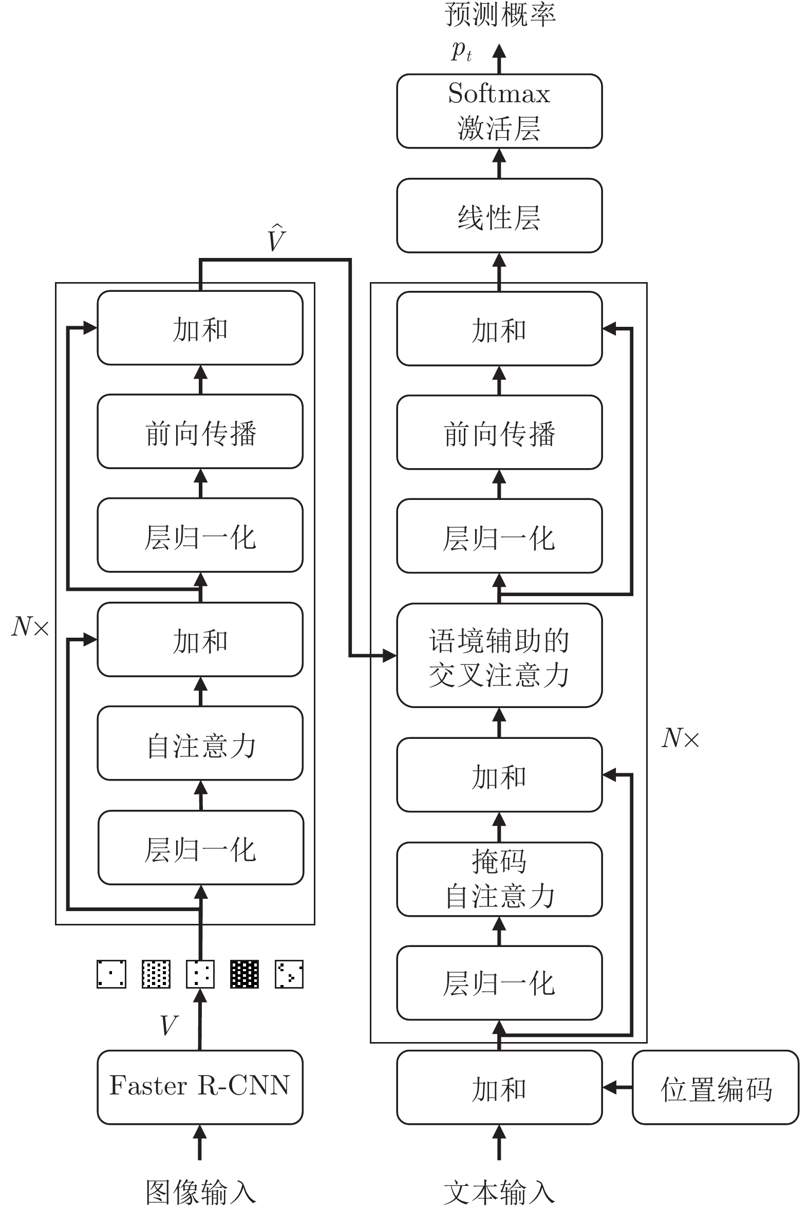
    图  2  语境辅助的交叉注意力机制与其轻量级的模型结构

    Fig.  2  Context-assisted cross attention mechanism and its light model structure

    图  3  基于语境辅助转换器的图像标题生成模型

    Fig.  3  Context-assisted transformer for image captioning

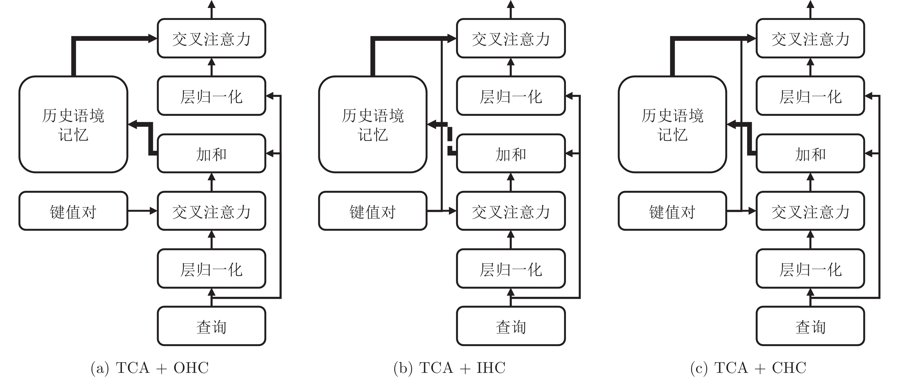
    图  4  传统交叉注意力机制的三种语境辅助策略

    Fig.  4  Three context-assisted strategies of traditional cross attention

    图  5  由语境辅助的交叉注意力模块分配给图像特征与历史语境记忆的注意力分布可视化

    Fig.  5  Visualization of attention distribution assigned to both image features and historical context memory by our CACA module

    图  6  Transformer与CAT生成的图像标题展示

    Fig.  6  Image captions generated by the Transformer and the CAT

    表  1  基于Transformer的图像标题生成模型结合(轻量级)语境辅助的交叉注意力机制在MS COCO数据集上的性能表现 (%)

    Table  1  Performance of Transformer-based image captioning models combined with (Light)CACA on MS COCO dataset (%)

    模型名称 BLEU-1 BLEU-4 METEOR ROUGE-L CIDEr-D SPICE
    Transformer 80.0 38.0 28.5 57.9 126.5 22.4
    Transformer + CACA (CAT) 80.8 38.9 28.9 58.6 129.6 22.6
    Transformer + LightCACA (LightCAT) 80.6 38.4 28.6 58.2 127.8 22.5
    $\mathcal{M}^{2}$Transformer[25] 80.8 39.1 29.2 58.6 131.2 22.6
    $\mathcal{M}^{2}$Transformer + CACA 81.2 39.4 29.5 59.0 132.4 22.8
    $\mathcal{M}^{2}$Transformer + LightCACA 81.2 39.3 29.4 58.8 131.9 22.8
    DLCT[27] 81.4 39.8 29.5 59.1 133.8 23.0
    DLCT + CACA 81.6 40.2 29.6 59.2 134.3 23.2
    DLCT + LightCACA 81.4 40.0 29.5 59.2 134.1 23.0
    $\mathcal{S}^{2}$Transformer[28] 81.1 39.6 29.6 59.1 133.5 23.2
    $\mathcal{S}^{2}$Transformer + CACA 81.5 40.0 29.7 59.3 134.2 23.3
    $\mathcal{S}^{2}$Transformer + LightCACA 81.3 39.7 29.6 59.3 133.8 23.3
    DIFNet[29] 81.7 40.0 29.7 59.4 136.2 23.2
    DIFNet + CACA 82.0 40.5 29.9 59.7 136.8 23.4
    DIFNet + LightCACA 81.9 40.1 29.7 59.5 136.4 23.2
    下载: 导出CSV

    表  2  基于LSTM的图像标题生成模型结合语境辅助的交叉注意力机制在MS COCO数据集上的性能表现 (%)

    Table  2  Performance of LSTM-based image captioning models combined with CACA on MS COCO dataset (%)

    模型名称 BLEU-1 BLEU-4 METEOR ROUGE-L CIDEr-D SPICE
    Att2in[31] 33.3 26.3 55.3 111.4
    Att2in + CACA 77.8 36.7 27.5 57.1 119.7 21.0
    BUTD[16] 79.8 36.3 27.7 56.9 120.1 21.4
    BUTD + CACA 80.4 38.1 28.3 58.2 126.4 22.1
    LB[10] 79.6 37.7 28.4 58.1 124.4 21.8
    LB + CACA 80.8 38.6 28.6 58.6 128.1 22.3
    下载: 导出CSV

    表  3  语境辅助的交叉注意力机制对Transformer推理效率的影响(ms)

    Table  3  The effect of context-assisted cross attention mechanism on Transformer's reasoning efficiency (ms)

    模型名称 单轮贪心解码时间 单轮集束搜索解码时间
    Transformer 4.7 63.9
    CAT 6.1 86.6
    LightCAT 4.9 68.1
    下载: 导出CSV

    表  4  本文模型与先进方法在MS COCO数据集上的性能对比(%)

    Table  4  Performance comparison between our models and the state-of-the-art (%)

    模型名称 BLEU-1 BLEU-4 METEOR ROUGE-L CIDEr-D SPICE
    Att2in[31] 33.3 26.3 55.3 111.4
    Att2all[31] 34.2 26.7 55.7 114.0
    BUTD[16] 79.8 36.3 27.7 56.9 120.1 21.4
    AoANet[18] 80.2 38.9 29.2 58.8 129.8 22.4
    $\mathcal{M}^{2}$Transformer[25] 80.8 39.1 29.2 58.6 131.2 22.6
    X-LAN[19] 80.8 39.5 29.5 59.2 132.0 23.4
    X-Transformer[19] 80.9 39.7 29.5 59.1 132.8 23.4
    DLCT[27] 81.4 39.8 29.5 59.1 133.8 23.0
    RSTNet (ResNext101)[26] 81.1 39.3 29.4 58.8 133.3 23.0
    BUTD + CATT[20] 38.6 28.5 58.6 128.3 21.9
    Transformer + CATT[20] 39.4 29.3 58.9 131.7 22.8
    $\mathcal{S}^{2}$Transformer[28] 81.1 39.6 29.6 59.1 133.5 23.2
    DIFNet[29] 81.7 40.0 29.7 59.4 136.2 23.2
    ${\rm{CIIC}}_{\mathcal{O}}$ [39] 81.4 40.2 29.3 59.2 132.6 23.2
    ${\rm{CIIC}}_{\mathcal{G}}$ [39] 81.7 40.2 29.5 59.4 133.1 23.2
    Transformer + CACA (CAT) 80.8 38.9 28.9 58.6 129.6 22.6
    $\mathcal{M}^{2}$Transformer + CACA 81.2 39.4 29.5 59.0 132.4 22.8
    DLCT + CACA 81.6 40.2 29.6 59.2 134.3 23.2
    $\mathcal{S}^{2}$Transformer + CACA 81.5 40.0 29.7 59.3 134.2 23.3
    DIFNet + CACA 82.0 40.5 29.9 59.7 136.8 23.4
    下载: 导出CSV

    表  5  传统交叉注意力机制结合不同语境辅助策略在MS COCO数据集上的表现(%)

    Table  5  Performance of the traditional cross attention mechanism combined with different context-assisted strategies on MS COCO dataset (%)

    模型名称 BLEU-1 BLEU-4 METEOR ROUGE-L CIDEr-D SPICE
    TCA (base) 80.0 38.0 28.5 57.9 126.5 22.4
    TCA + OHC 80.4 37.8 28.2 57.4 126.8 21.8
    TCA + IHC 80.8 38.2 28.5 58.1 128.2 22.2
    TCA + CHC (CACA) 81.2 38.6 28.6 58.2 128.9 22.6
    下载: 导出CSV

    表  6  不同解码器层数的CAT模型在共享与不共享交叉注意力模块参数时的性能表现(%)

    Table  6  Performance of CAT models with different decoder layers when sharing or not sharing parameters of the cross attention module (%)

    解码器层数 交叉注意力模块设置 BLEU-1 BLEU-4 METEOR ROUGE-L CIDEr-D SPICE
    $N=2$ TCA 78.8 37.4 28.0 57.4 125.4 21.8
    $N=2$ CACA (Shared) 80.4 38.0 28.2 57.8 128.0 22.3
    $N=2$ CACA (Not shared) 80.8 38.4 28.5 58.2 128.8 22.5
    $N=3$ TCA 80.0 38.0 28.5 57.9 126.5 22.4
    $N=3$ CACA (Shared) 81.2 38.6 28.6 58.2 128.9 22.6
    $N=3$ CACA (Not shared) 81.0 38.8 28.8 58.3 129.3 22.7
    $N=4$ TCA 79.6 37.8 28.5 57.8 126.2 22.2
    $N=4$ CACA (Shared) 79.8 37.5 28.4 57.6 125.8 21.9
    $N=4$ CACA (Not shared) 79.0 36.8 28.1 57.1 124.3 21.5
    下载: 导出CSV

    表  7  采用自适应权重约束的CAT模型在MS COCO数据集上的表现(%)

    Table  7  Performance of the CAT model with adaptive weight constraint on MS COCO dataset (%)

    权重约束方式 BLEU-4 METEOR ROUGE-L CIDEr-D
    无权重约束 38.6 28.6 58.2 128.9
    固定权重约束$\beta=0.1$ 38.4 28.4 58.1 127.8
    固定权重约束$\beta=0.3$ 38.7 28.6 58.3 128.7
    固定权重约束$\beta=0.5$ 38.9 28.7 58.4 129.3
    固定权重约束$\beta=0.7$ 38.5 28.4 58.1 128.4
    固定权重约束$\beta=0.9$ 38.1 28.2 57.6 127.2
    自适应权重约束 38.9 28.9 58.6 129.6
    下载: 导出CSV

    表  8  Transformer与CAT模型的人工评价(%)

    Table  8  Human evaluation of Transformer and CAT (%)

    模型名称 更强的相关性 更强的一致性
    Transformer 8.8 7.4
    CAT 10.2 12.4
    下载: 导出CSV
  • [1] Ji J, Luo Y, Sun X, Chen F, Luo G, Wu Y, et al. Improving image captioning by leveraging intra- and inter-layer global representation in Transformer network. In: Proceedings of the AAAI Conference on Artificial Intelligence. Virtual Conference: 2021. 1655−1663
    [2] Fang Z, Wang J, Hu X, Liang L, Gan Z, Wang L, et al. Injecting semantic concepts into end-to-end image captioning. In: Proceedings of the IEEE/CVF Conference on Computer Vision and Pattern Recognition. New Orleans, Louisiana, USA: IEEE, 2022. 18009−18019
    [3] Tan J H, Tan Y H, Chan C S, Chuah J H. Acort: a compact object relation transformer for parameter efficient image captioning. Neurocomputing, 2022, 482: 60-72 doi: 10.1016/j.neucom.2022.01.081
    [4] Fei Z. Attention-aligned Transformer for image captioning. In: Proceedings of the AAAI Conference on Artificial Intelligence. Vancouver, British Columbia, Canada: 2022. 607−615
    [5] Stefanini M, Cornia M, Baraldi L, Cascianelli S, Fiameni G, Cucchiara R. From show to tell: a survey on deep learning-based image captioning. IEEE Transactions on Pattern Analysis and Machine Intelligence, 2022, 45(1): 539-559
    [6] Vinyals O, Toshev A, Bengio S, Erhan D. Show and tell: lessons learned from the 2015 mscoco image captioning challenge. IEEE Transactions on Multimedia, 2016, 39(4): 652-663
    [7] Vaswani A, Shazeer N, Parmar N, Uszkoreit J, Jones L, Gomez A N, et al. Attention is all you need. In: Proceedings of Advances in Neural Information Processing Systems. Long Beach, USA: 2017. 5998−6008
    [8] Cover T M, Thomas J A. Elements of Information Theory. New York: John Wiley & Sons, 2012.
    [9] Lin T Y, Maire M, Belongie S J, Hays J, Perona P, Ramanan D, et al. Microsoft coco: Common objects in context. In: Proceedings of European Conference on Computer Vision. Zurich, Switzerland: 2014. 740−755
    [10] Qin Y, Du J, Zhang Y, Lu H. Look back and predict forward in image captioning. In: Proceedings of the IEEE/CVF Conference on Computer Vision and Pattern Recognition. Long Beach, USA: IEEE, 2019. 8367−8375
    [11] Aneja J, Deshpande A, Schwing A G. Convolutional image captioning. In: Proceedings of the IEEE/CVF Conference on Computer Vision and Pattern Recognition. Salt Lake City, Utah, USA: IEEE, 2018. 5561−5570
    [12] 汤鹏杰, 王瀚漓, 许恺晟. LSTM逐层多目标优化及多层概率融合的图像描述. 自动化学报, 2018, 44(7): 1237-1249

    Tang Peng-Jie, Wang Han-Li, Xu Kai-Sheng. Multi-objective layer-wise optimization and multi-level probability fusion for image description generation using lstm. Acta Automatica Sinica, 2018, 44(7): 1237-1249
    [13] Xu K, Ba J, Kiros R, Cho K, Courville A C, Salakhutdinov R, et al. Show, attend and tell: Neural image caption generation with visual attention. In: Proceedings of the 32nd International Conference on Machine Learning. Lille, France: 2015. 2048−2057
    [14] You Q, Jin H, Wang Z, Fang C, Luo J. Image captioning with semantic attention. In: Proceedings of the IEEE/CVF Conference on Computer Vision and Pattern Recognition. Las Vegas, Nevada, USA: 2016. 4651−4659
    [15] Lu J, Xiong C, Parikh D, Socher R. Knowing when to look: Adaptive attention via a visual sentinel for image captioning. In: Proceedings of the IEEE/CVF Conference on Computer Vision and Pattern Recognition. Hawaii, USA: IEEE, 2017. 3242−3250
    [16] Anderson P, He X, Buehler C, Teney D, Johnson M, Gould S, et al. Bottom-up and top-down attention for image captioning and visual question answering. In: Proceedings of the IEEE/CVF Conference on Computer Vision and Pattern Recognition. Salt Lake City, Utah, USA: IEEE, 2018. 6077−6086
    [17] Chen S, Zhao Q. Boosted attention: Leveraging human attention for image captioning. In: Proceedings of European Conference on Computer Vision. Munich, Germany: 2018. 68−84
    [18] Huang L, Wang W, Chen J, Wei X. Attention on attention for image captioning. In: Proceedings of the IEEE/CVF International Conference on Computer Vision. Seoul, South Korea: IEEE, 2019. 4633−4642
    [19] Pan Y, Yao T, Li Y, Mei T. X-linear attention networks for image captioning. In: Proceedings of the IEEE/CVF Conference on Computer Vision and Pattern Recognition. Seattle, USA: IEEE, 2020. 10968−10977
    [20] Yang X, Zhang H, Qi G, Cai J. Causal attention for vision-language tasks. In: Proceedings of the IEEE/CVF Conference on Computer Vision and Pattern Recognition. Virtual Conference: 2021. 9847−9857
    [21] 王鑫, 宋永红, 张元林. 基于显著性特征提取的图像描述算法. 自动化学报, 2022, 48(3): 735-746

    Wang Xin, Song Yong-Hong, Zhang Yuan-Lin. Salient feature extraction mechanism for image captioning. Acta Automatica Sinica, 2022, 48(3): 735-746
    [22] Herdade S, Kappeler A, Boakye K, Soares J. Image captioning: transforming objects into words. In: Proceedings of Advances in Neural Information Processing Systems. Vancouver, Canada: 2019. 11135−11145
    [23] Li G, Zhu L, Liu P, Yang Y. Entangled transformer for image captioning. In: Proceedings of the IEEE/CVF International Conference on Computer Vision. Seoul, South Korea: IEEE, 2019. 8927−8936
    [24] Yu J, Li J, Yu Z, Huang Q. Multimodal transformer with multi-view visual representation for image captioning. IEEE Transactions on Circuits and Systems for Video Technology, 2019, 30(12): 4467-4480
    [25] Cornia M, Stefanini M, Baraldi L, Cucchiara R. Meshed-memory transformer for image captioning. In: Proceedings of the IEEE/CVF Conference on Computer Vision and Pattern Recognition. Seattle, USA: IEEE, 2020. 10575−10584
    [26] Zhang X, Sun X, Luo Y, Ji J, Zhou Y, Wu Y, et al. Rstnet: Captioning with adaptive attention on visual and non-visual words. In: Proceedings of the IEEE/CVF Conference on Computer Vision and Pattern Recognition. Virtual Conference: 2021. 15465−15474
    [27] Luo Y, Ji J, Sun X, Cao L, Wu Y, Huang F, et al. Dual-level collaborative transformer for image captioning. In: Proceedings of the AAAI Conference on Artificial Intelligence. Virtual Conference: 2021. 2286−2293
    [28] Zeng P, Zhang H, Song J, Gao L. S2 transformer for image captioning. In: Proceedings of the International Joint Conferences on Artificial Intelligence. Vienna, Austria: 2022.
    [29] Wu M, Zhang X, Sun X, Zhou Y, Chen C, Gu J, et al. Difnet: Boosting visual information flow for image captioning. In: Proceedings of the IEEE/CVF Conference on Computer Vision and Pattern Recognition. New Orleans, Louisiana, USA: 2022. 18020−18029
    [30] Lian Z, Li H, Wang R, Hu X. Enhanced soft attention mechanism with an inception-like module for image captioning. In: Proceedings of the 32nd International Conference on Tools With Artificial Intelligence. Virtual Conference: 2020. 748−752
    [31] Rennie S J, Marcheret E, Mroueh Y, Ross J, Goel V. Self-critical sequence training for image captioning. In: Proceedings of the IEEE/CVF Conference on Computer Vision and Pattern Recognition. Hawaii, USA: 2017. 1179−1195
    [32] Vedantam R, Zitnick C L, Parikh D. Cider: Consensus-based image description evaluation. In: Proceedings of the IEEE/CVF Conference on Computer Vision and Pattern Recognition. Boston, USA: 2015. 4566−4575
    [33] Karpathy A, Li F F. Deep visual-semantic alignments for generating image descriptions. In: Proceedings of the IEEE/CVF Conference on Computer Vision and Pattern Recognition. Boston, USA: 2015. 3128−3137
    [34] Papineni K, Roukos S, Ward T, Zhu W J. Bleu: A method for automatic evaluation of machine translation. In: Proceedings of the 40th Annual Meeting of the Association for Computational Linguistics. Philadelphia, USA: 2002. 311−318
    [35] Denkowski M J, Lavie A. Meteor universal: Language specific translation evaluation for any target language. In: Proceedings of the 9th Workshop on Statistical Machine Translation. Baltimore, Maryland, USA: 2014. 376−380
    [36] Lin C Y. Rouge: A package for automatic evaluation of summaries. In: Proceedings of Workshop on Text Summarization Branches Out, Post-Conference Workshop of ACL 2004. Barcelona, Spain: 2004. 74−81
    [37] Anderson P, Fernando B, Johnson M, Gould S. Spice: Semantic propositional image caption evaluation. In: Proceedings of European Conference on Computer Vision. Amsterdam, Netherlands: 2016. 382−398
    [38] Krishna R, Zhu Y, Groth O, Johnson J, Hata K, Kravitz J, et al. Visual genome: connecting language and vision using crowdsourced dense image annotations. International Journal of Computer Vision, 2017, 123(1): 32-73 doi: 10.1007/s11263-016-0981-7
    [39] Liu B, Wang D, Yang X, Zhou Y, Yao R, Shao Z, et al. Show, deconfound and tell: Image captioning with causal inference. In: Proceedings of the IEEE/CVF Conference on Computer Vision and Pattern Recognition. New Orleans, Louisiana, USA: 2022. 18041−18050
  • 期刊类型引用(1)

    1. 蒋祥龙,顾传青. Thiele型张量连分式插值及其在张量指数计算中的应用. 上海大学学报(自然科学版). 2021(04): 650-658 . 百度学术

    其他类型引用(0)

  • 加载中
图(6) / 表(8)
计量
  • 文章访问数:  498
  • HTML全文浏览量:  122
  • PDF下载量:  156
  • 被引次数: 1
出版历程
  • 收稿日期:  2022-09-26
  • 录用日期:  2023-02-10
  • 网络出版日期:  2023-03-09
  • 刊出日期:  2023-09-26

目录

/

返回文章
返回