-
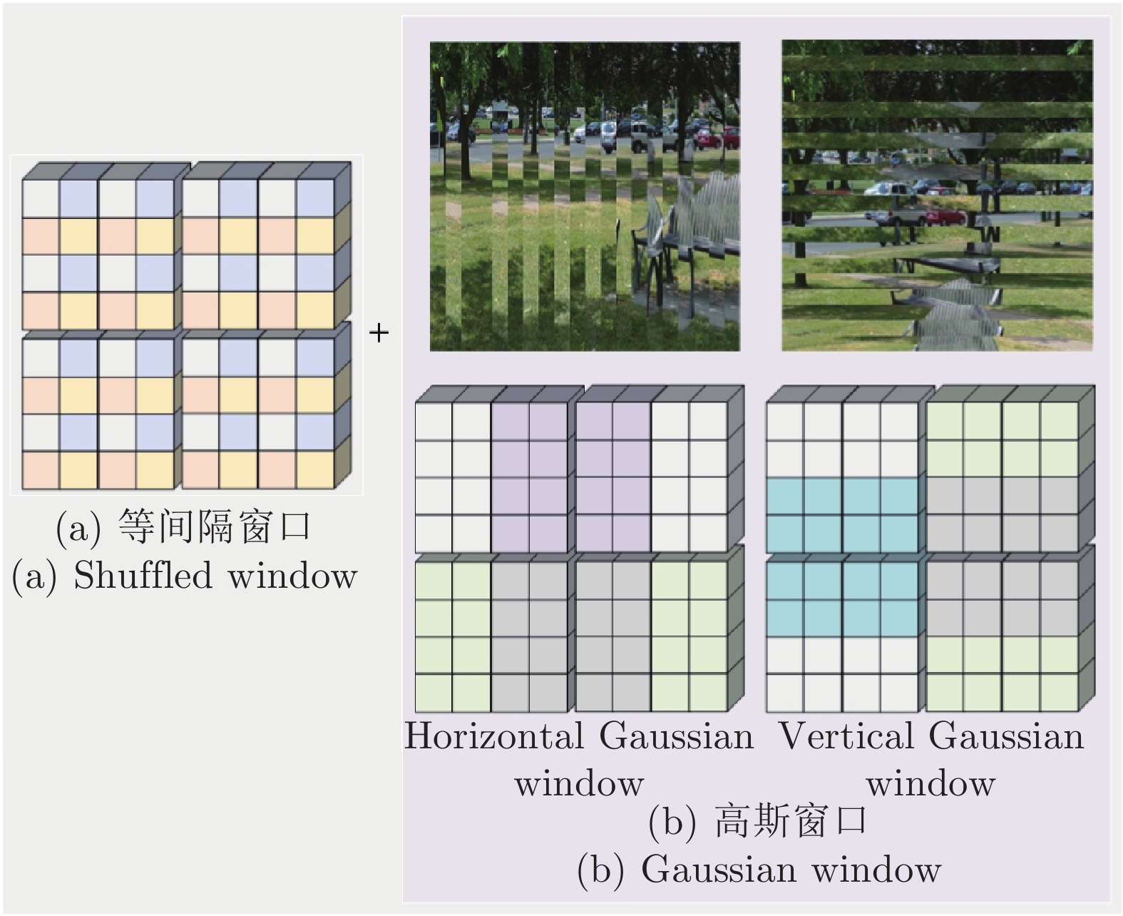
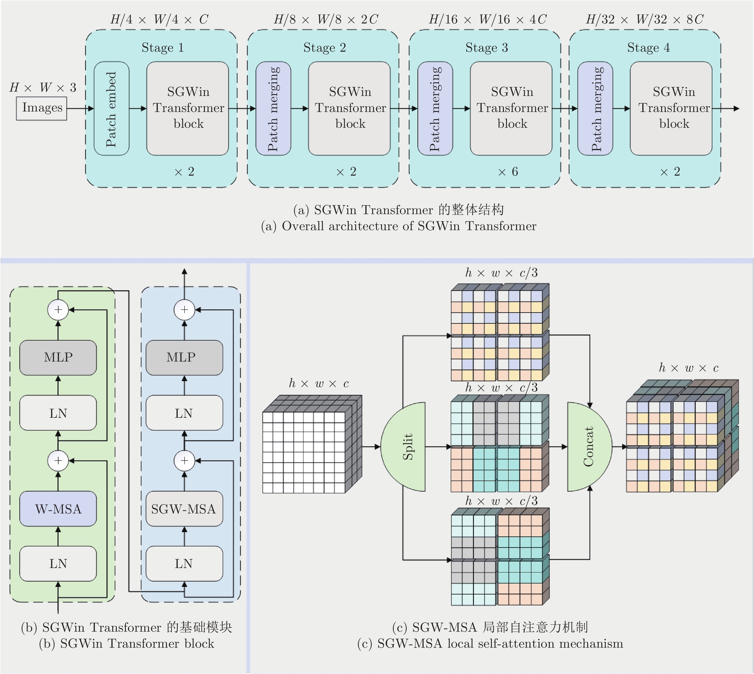
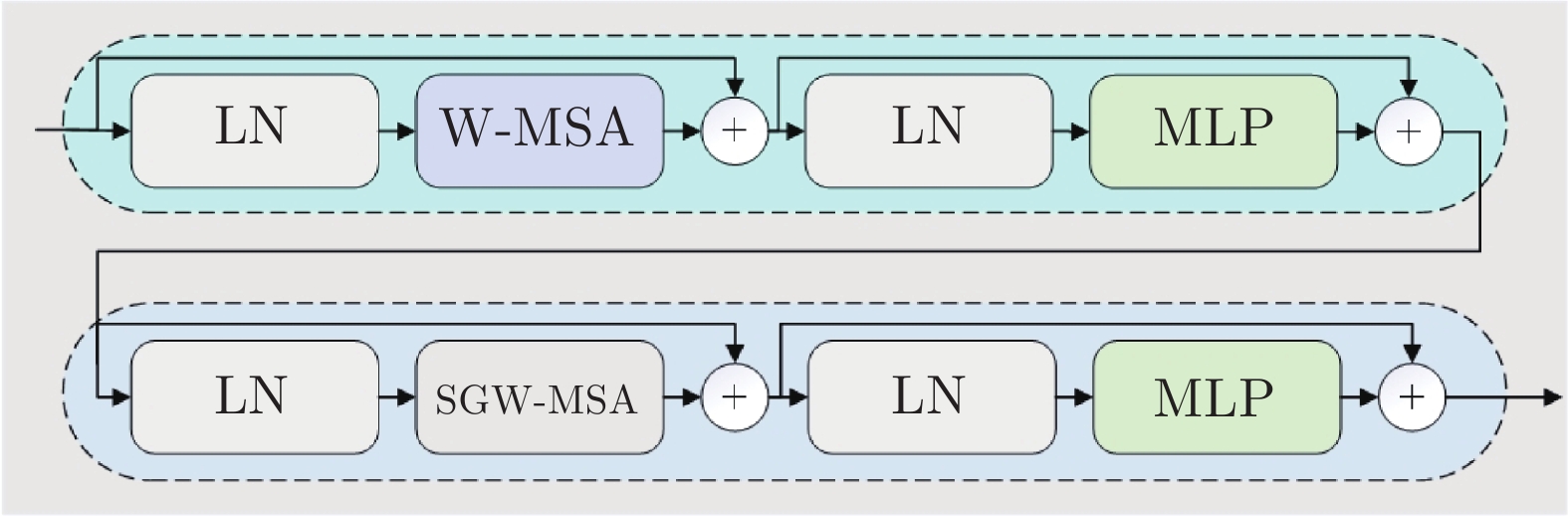
摘要: 在目前视觉Transformer的局部自注意力中, 现有的策略无法建立所有窗口之间的信息流动, 导致上下文语境建模能力不足. 针对这个问题, 基于混合高斯权重重组(Gaussian weight recombination, GWR)的策略, 提出一种新的局部自注意力机制SGW-MSA (Shuffled and Gaussian window-multi-head self-attention), 它融合了3种不同的局部自注意力, 并通过GWR策略对特征图进行重建, 在重建的特征图上提取图像特征, 建立了所有窗口的交互以捕获更加丰富的上下文信息. 基于SGW-MSA设计了SGWin Transformer整体架构. 实验结果表明, 该算法在mini-imagenet图像分类数据集上的准确率比Swin Transformer提升了5.1%, 在CIFAR10图像分类实验中的准确率比Swin Transformer提升了5.2%, 在MS COCO数据集上分别使用Mask R-CNN和Cascade R-CNN目标检测框架的mAP比Swin Transformer分别提升了5.5%和5.1%, 相比于其他基于局部自注意力的模型在参数量相似的情况下具有较强的竞争力.
-
关键词:
- Transformer /
- 局部自注意力 /
- 混合高斯权重重组 /
- 图像分类 /
- 目标检测
Abstract: In the current vision Transformer's local self-attention, the existing strategy cannot establish the information flow between all windows, resulting in the lack of context modeling ability. To solve this problem, this paper proposes a new local self-attention mechanism shuffled and Gaussian window-multi-head self-attention (SGW-MSA) based on the strategy of Gaussian weight recombination (GWR), which combines three different local self-attention forces, and reconstructs the feature map through GWR strategy, and extracts image features from the reconstructed feature map. The interaction of all windows is established to capture richer context information. This paper designs the overall architecture of SGWin Transformer based on SGW-MSA. The experimental results show that the accuracy of this algorithm in the mini-imagenet image classification dataset is 5.1% higher than that in the Swin Transformer, the accuracy in the CIFAR10 image classification experiment is 5.2% higher than that in the Swin Transformer, and the mAP using the Mask R-CNN and Cascade R-CNN object detection frameworks on the MS COCO dataset are 5.5% and 5.1% higher than that in the Swin Transformer, respectively. Compared with other models based on local self-attention, it has stronger competitiveness in the case of similar parameters. -
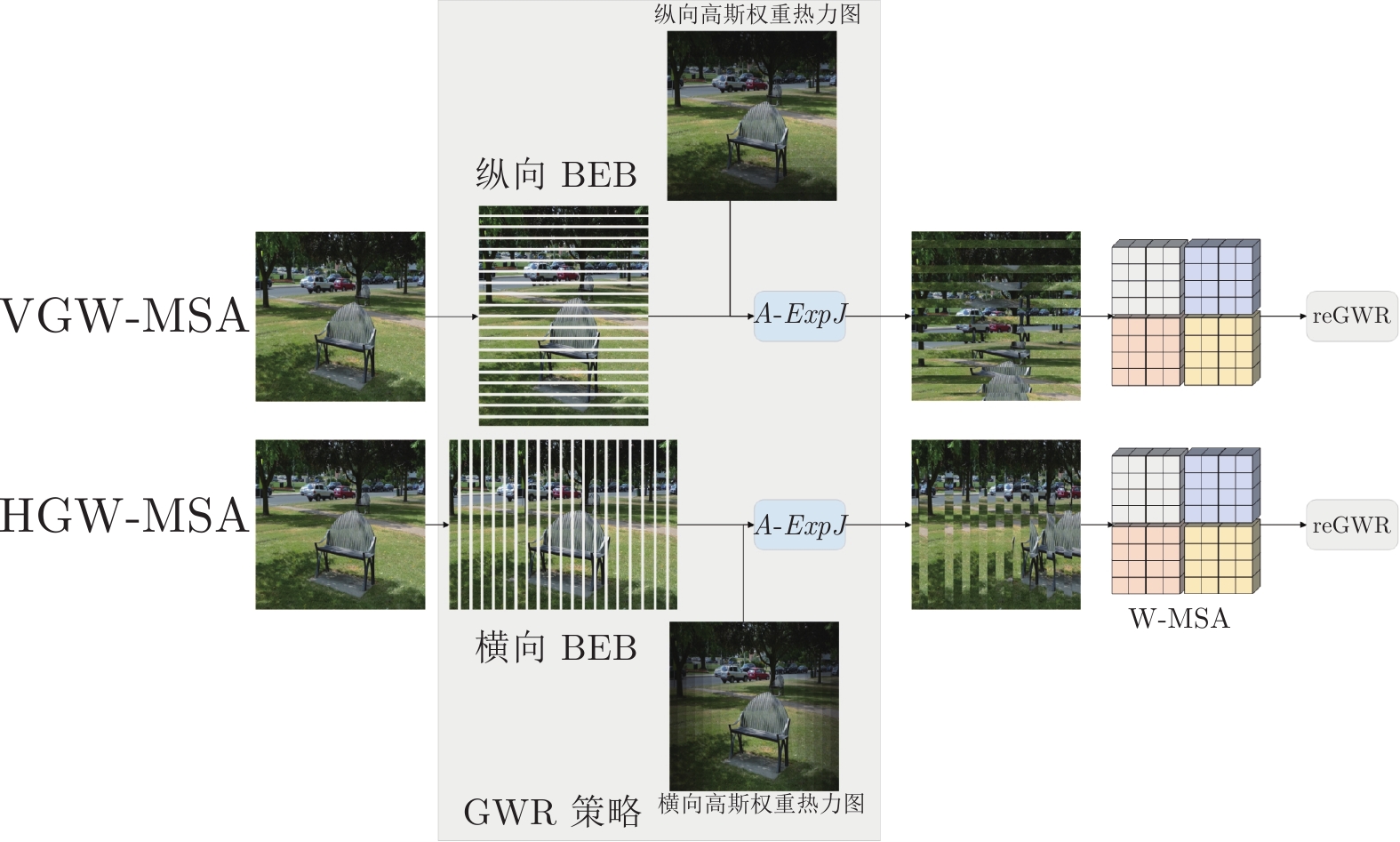
近年来, 张量方法在控制理论及其应用的各个领域得到了广泛的应用, 如基于张量数据表示的深度学习模型[1]、基于非负张量分析的时序链路预测方法[2]、局部图像描述中基于结构张量的HDO (Histograms of dominant orientations)算法[3]、二维解析张量投票算法[4]等.
张量动力系统已经广泛应用于Volterra系统识别[5]、张量乘积TP (Tensor product)模型变换[6]、人体动作识别[7-8]和塑性模型[9]等各个领域.因此, 由于在张量常微分方程解中的关键作用, 张量指数函数的计算已经成为一个重要的研究领域.
考虑如下常微分方程[9]
$$ \begin{align}\label{equation1-1} \left\{ \begin{array}{ll} \dot{\mathcal{Y}}(t)=\mathcal{A}\mathcal{Y}(t) \\ {\mathcal{Y}}(t_0)=\mathcal{Y}_{0} \end{array} \right. \end{align} $$ (1) 这里$\mathcal{A}$和$\mathcal{Y}_{0}$是给定张量, 一般是非对称的, 那么关于系统(1)的张量指数函数${\rm exp}(\cdot)$有如下唯一解:
$$ \begin{align}\label{equation1-2} {\mathcal{Y}}(t)={\rm exp}[(t-t_0)\mathcal{A}]{\mathcal{Y}}_{0} \end{align} $$ (2) 对于一般的张量$\mathcal{A}$, 它的指数函数可以表示为它的级数形式:
$$ \begin{align*}{\rm exp}(\mathcal{A})=\sum\limits_{n=0}^\infty \frac{1}{n!}\mathcal{A}^n\end{align*} $$ 目前计算张量指数函数(2)通常使用的方法是截断法[10], 其实质就是将张量指数函数展开成无穷级数后, 取前$n_{\rm{max}}$项, 得到近似解, 即:
$$ \begin{align*}{\rm exp}(\mathcal{A}) \approx \sum\limits_{n=0}^{n_{\rm{max}}} \frac{1}{n!}\mathcal{A}^n\end{align*} $$ 张量指数函数选取的项数$n_{\rm{max}}$受限于所需的精度:
$$ \begin{align*}\frac{1}{n_{\rm{max}}!}\|\mathcal{A}^{n_{\rm{max}}}\|\le \epsilon_{\rm{tol}}\end{align*} $$ 显然有截断法的精度与张量指数函数选取的项数$n_{\rm{max}}$有关, 保留的项数越多, 精度越高, 但是需要进行的张量乘积次数也就越多; 保留的项数越少, 计算量越少, 但是精度也就越低.因此, 计算张量指数函数的截断法有待改进.
为研究上述问题, 本文首次定义了张量的一种广义逆, 并以此为基础构造了张量广义逆Padé逼近GITPA (Generalized inverse tensor Padé approximation)的一种$\varepsilon$-算法. GITPA方法的优势在于:在计算过程中, 不必用到张量的乘积, 也不要计算张量的逆, 另外, 该方法对奇异张量也是适用的.目前在国内外, 关于计算张量的逆还没有找到一种比较可行的计算方法.作为GITPA方法的一个重要应用, 本文在后面给出计算张量指数函数的数值实验, 来说明$\varepsilon$-算法的有效性.
本文组织如下:第1节简单介绍本文用到的张量基础知识, 并定义张量的一种广义逆; 第2节, 首先给出广义逆张量Padé逼近的定义, 并以此为基础给出张量$\varepsilon$-算法; 第3节将$\varepsilon$-算法用来计算张量指数函数值, 并与通常使用的的级数截断法相比较; 最后给出简单的小结.
1. 一种张量广义逆
1.1 张量基础知识
本节介绍本文将要用到的张量基础知识.张量是一种多维数组, 其中向量是一阶张量, 矩阵是二阶张量, 特别地, 一个$ p $阶张量拥有$ p $个下标, 是$ p $个拥有独立坐标系的向量空间的外积(张量积).一个$ p $阶$ n_1\times n_2\times \cdots \times n_p $维张量可以表示为:
$$ \mathcal{A} = (a_{i_{1}i_{2}\cdots i_{p}})\in {\bf C}^{n_{1}\times n_{2}\times\cdots \times n_{p}} $$ 文献[11]提出了张量的切片方法.对一个三阶张量, 可以固定其中任意一个下标, 从而得到该张量的一种表示形式.设$ \mathcal{A} = (a_{i_{1}i_{2}i_{3}})\in {\bf C}^{2\times 2\times3} $, 固定其第三个下标, 则张量可以表示为
$$ \begin{align*} \mathcal{A} = \, &\left[ \begin{array}{c|c|c} \mathcal{A}_{1} &\mathcal{A}_{2}& \mathcal{A}_{3} \end{array}\right] = \nonumber\\ &\left[ \begin{array}{cc|cc|cc} a_{111} & a_{121} & a_{112} & a_{122} & a_{113} & a_{123}\\ a_{211} & a_{221} & a_{212} & a_{222} & a_{213} & a_{223}\\ \end{array} \right] \end{align*} $$ 下面定义两个三阶张量的$ t $-积, 可以通过递归自然地推广到高阶张量的$ t $-积.
定义1[12]. (块循环矩阵)令$ \mathcal{A} \in {\bf R}^{l\times p\times n} $, 则$ \mathcal{A} $的块循环矩阵被定义为
$$ \begin{equation*} bcirc(\mathcal{A}) = {\left[ \begin{array}{ccccc} \mathcal{A}_{1} & \mathcal{A}_{n} & \mathcal{A}_{n-1} & \cdots & \mathcal{A}_{2} \\ \mathcal{A}_{2} & \mathcal{A}_{1} & \mathcal{A}_{n} & \cdots & \mathcal{A}_{3} \\ \vdots & \vdots & \vdots & \ddots & \vdots \\ \mathcal{A}_{n} & \mathcal{A}_{n-1} & \cdots & \mathcal{A}_{2} & \mathcal{A}_{1} \\ \end{array} \right]}_{ln\times pn} \end{equation*} $$ 定义一个展开算子: $ unfold(\cdot)$[12], 用以下方式将一个${p\times m\times n}$的张量展开成一个${pn\times m}$的矩阵:
$$ \begin{equation*} unfold(\mathcal{B}) = \left[ \begin{array}{c} \mathcal{B}_{1}^{\rm{T}} \mathcal{B}_{2}^{\rm{T}} \cdots \mathcal{B}_{n}^{\rm{T}}\\ \end{array} \right]^{\rm{T}} \end{equation*} $$ 这里$fold(\cdot)$[12]是它的逆算子, 它会将一个$ {pn\times m} $的矩阵转化成$ {p\times m\times n} $的张量.因此,
$$ \begin{equation*} fold(unfold(\mathcal{B})) = \mathcal{B} \end{equation*} $$ 定义2[12-13]. (张量$ t $-积)令$ \mathcal{A} $是一个$ l\times p\times n $的张量, $ \mathcal{B} $是一个$ p\times m\times n $的张量, 则张量$ t $-积$ \mathcal{A}*\mathcal{B} $将得到一个$ l\times m\times n $的张量, 定义如下:
$$ \begin{equation*} \mathcal{A}\ast \mathcal{B} = fold(bcirc(\mathcal{A}) \cdot unfold(B)) \end{equation*} $$ 例1. 设$ \mathcal{A}, \mathcal{B}\in {\bf R}^{2\times 2\times3} $, 现固定其第三个下标, 分别产生
$$ \begin{align*} \begin{array}{rl} \mathcal{A} = &\left[ \begin{array}{cc|cc|cc} 1 & 2 & 5 & 6 & 9 & 10 \\ 3 & 4 & 7 & 8 & 11 & 12 \\ \end{array} \right]\\ \mathcal{B} = &\left[ \begin{array}{cc|cc|cc} 1 & 2 & 4 & 3 & 1 & 0 \\ 3 & 4 & 2 & 1 & 0 & 1 \\ \end{array} \right]\end{array} \end{align*} $$ 则由定义2得到
$$ \begin{align*} \begin{array}{rl} \mathcal{A}\ast\! \mathcal{B} = \\&fold\left[ \begin{array}{c} \left[ \begin{array}{ccc} \mathcal{A}_{1} & \mathcal{A}_{3} & \mathcal{A}_{2} \\ \mathcal{A}_{2} & \mathcal{A}_{1} & \mathcal{A}_{3} \\ \mathcal{A}_{3} & \mathcal{A}_{2} & \mathcal{A}_{1} \\ \end{array} \right]\cdot\left[ \begin{array}{c} \mathcal{B}_{1} \\ \mathcal{B}_{2} \\ \mathcal{B}_{3} \\ \end{array} \right] \\ \end{array} \right] = \\ &fold\left[ \begin{array}{c} \mathcal{A}_{1}\mathcal{B}_{1}+\mathcal{A}_{3}\mathcal{B}_{2}+\mathcal{A}_{2}\mathcal{B}_{3} \\ \mathcal{A}_{2}\mathcal{B}_{1}+\mathcal{A}_{1}\mathcal{B}_{2}+\mathcal{A}_{3}\mathcal{B}_{3} \\ \mathcal{A}_{3}\mathcal{B}_{1}+\mathcal{A}_{2}\mathcal{B}_{2}+\mathcal{A}_{1}\mathcal{B}_{3} \\ \end{array} \right] = \\ &\left[ \begin{array}{cc|cc|cc} 68 & 53 & 40 & 49 & 72 & 81 \\ 90 & 75 & 62 & 71 & 94 & 103 \\ \end{array} \right] \end{array} \end{align*} $$ 下面定义张量的范数.令$ \mathcal{A}\in {\bf C}^{n_{1}\times n_{2}\times\cdots \times n_{p}} $, 张量的范数就等于它所有元素平方和的平方根[11], 即
$$ \begin{align} \|\mathcal{A}\| = \sqrt{\sum^{n_{1}}_{i_{1} = 1}\sum^{n_{2}}_{i_{2} = 1}\cdots\sum^{n_{p}}_{i_{p} = 1}a^2_{i_{1}i_{2}\cdots i_{p}}} \end{align} $$ (3) 这和矩阵的$ Frobenius $-模是类似的.两个大小相同的张量$ \mathcal{A} $, $ \mathcal{B}\in {\bf C}^{n_{1}\times n_{2}\times\cdots \times n_{p}} $的内积等于它们对应元素的乘积的和[11], 即
$$ \begin{align} (\mathcal{A}, \mathcal{B}) = \sum^{n_{1}}_{i_{1} = 1}\sum^{n_{2}}_{i_{2} = 1}\cdots\sum^{n_{p}}_{i_{p} = 1}a_{i_{1}i_{2}\cdots i_{p}}b_{i_{1}i_{2}\cdots i_{p}} \end{align} $$ (4) 于是显然成立$ (\mathcal{A}, \mathcal{A}^\ast) = \|\mathcal{A}\|^2 $, 其中记号"$ \ast $''表示取复共轭.
1.2 张量广义逆
参考复数、向量和矩阵的倒数, 容易得到以下结论:
1) 若$ b $是一个复数, $ b\in {\bf C} $, 则$ bb^\ast = |b|^2 $, $ {1}/{b} = b^{-1} = {b^\ast}/{|b|^2} $;
2) 若$ {\pmb v} $是一个向量, $ {\pmb v}\in {\bf C}^n $, 则$ {\pmb v}\cdot {\pmb v}^\ast = |{\pmb v}|^2 $, $ {1}/{{\pmb v}} = {\pmb v}^{-1} = {{\pmb v}^\ast}/{|{\pmb v}|^2} $ (见Graves-Morris [14]);
3) 若$ A = a_{ij} $, $ B = b_{ij}\in {\bf C}^{s\times t} $, 则$ A\cdot B = \sum^s_{i = 1}\sum^t_{j = 1}(a_{ij}b_{ij})\in {\bf C} $, $ {1}/{A} = A_r^{-1} = {A^\ast}{\|A\|^2} $ (见顾传青[15-17]).因此, 下面张量的广义逆可以看作是向量和矩阵的推广:
定义3. 令$ \mathcal{A}, \mathcal{B}\in {\bf C}^{n_1\times n_2\times \cdots\times n_p} $, 其内积为
$$ \begin{equation*} (\mathcal{A}, \mathcal{B}) = \sum\limits^{n_{1}}_{i_{1} = 1}\sum\limits^{n_{2}}_{i_{2} = 1}\cdots\sum\limits^{n_{p}}_{i_{p} = 1}a_{i_{1}i_{2}\cdots i_{p}b_{i_{1}i_{2}\cdots i_{p}}} \end{equation*} $$ $ \mathcal{A}\cdot\mathcal{A}^\ast = \parallel\mathcal{A}\parallel^2 $, 则张量$ \mathcal{A} $的广义逆被定义为
$$ \begin{align} \begin{aligned} \mathcal{A}_r^{-1}& = \frac{1}{\mathcal{A}} = \frac{\mathcal{A}^\ast}{\parallel\mathcal{A}\parallel^2}, \mathcal{A}\neq 0, \mathcal{A}\in {\bf C}^{n_1\times n_2\times \cdots\times n_p} \end{aligned} \end{align} $$ (5) 其中张量的范数由式(3)给出.
引理1. 令$ \mathcal{A}, \mathcal{B}\in {\bf C}^{n_1\times n_2\times \cdots\times n_p}, \mathcal{A}, \mathcal{B}\neq0 $且$ b\in {\bf R}, b\neq0 $, 则下列关系成立:
1) $ \frac{b}{\mathcal{A}} = \frac{1}{\mathcal{B}}\Longleftrightarrow\mathcal{A} = b\mathcal{B} $;
2) $ (\mathcal{A}^{-1}_r)^{-1}_r = \mathcal{A}, (b\mathcal{A})^{-1}_r = \frac{1}{b}\mathcal{A}^{-1}_r $.
证明. 根据定义3, 结论2)是显然的.现在证明结论1).因为$ \mathcal{A}, \mathcal{B}\neq0 $, 从$ \mathcal{A} = b\mathcal{B} $, 容易推得$ \frac{b}{\mathcal{A}} = \frac{1}{\mathcal{B}} $.利用定义3, 得到引理1的左端, $ \frac{b\mathcal{A}^\ast}{\|\mathcal{A}\|^2} = \frac{\mathcal{B}^\ast}{\|\mathcal{B}\|^2} $, 即
$$ \begin{align*} \mathcal{A}^\ast = \frac{\parallel\mathcal{A}\parallel^2}{b\parallel\mathcal{B}\parallel^2}\mathcal{B}^\ast, \mathcal{A} = \frac{\parallel\mathcal{A}\parallel^2}{b\parallel\mathcal{B}\parallel^2}\mathcal{B} \end{align*} $$ 因此
$$ \begin{align*} \parallel\mathcal{A}\parallel^2 = \mathcal{A}\cdot\mathcal{A}^\ast = \frac{\parallel\mathcal{A}\parallel^4\parallel\mathcal{B}\parallel^2}{b^2\parallel\mathcal{B}\parallel^4} \end{align*} $$ 即$ b^2 = \frac{\parallel\mathcal{A}\parallel^2}{\parallel\mathcal{B}\parallel^2} $, 所以$ \mathcal{A} = b\mathcal{B} $.
2. 张量广义逆$ \pmb{\varepsilon} $-算法
2.1 广义逆张量Padé逼近的定义
设$ f(t) $是给定的张量多项式, 其系数为张量, 即
$$ \begin{equation} f(t) = \mathcal{C}_0+\mathcal{C}_1t+\mathcal{C}_2t^2+\cdots+\mathcal{C}_nt^n+\cdots \end{equation} $$ (6) $$ \begin{equation*} \mathcal{C}_i = (c_i^{(i_1i_2\cdots i_p)})\in {\bf C}^{n_{1}\times n_{2}\times\cdots \times n_{p}}, t\in {\bf C} \end{equation*} $$ 定义4. 令$ C^{n_1\times n_2\times \cdots\times n_p}[t] $是一个$ p $阶张量的多项式集合, 维数分别为$ n_1\times n_2\times \cdots\times n_p $.一个张量多项式$ \mathcal{A}(t) = (a_{i_1i_2 \cdots i_p}(t))\in {\bf C}^{n_1\times n_2\times \cdots\times n_p}[t] $是$ m $阶的, 表示为$ \partial\mathcal{A}(t) = m $, 若$ \partial(a_{i_1i_2 \cdots i_p}(t))\leq m $对于所有$ i_i = 1, 2, \cdots, n_i, 1\leq i\leq p $都成立, 且$ \partial(a_{(i_1i_2 \cdots i_p)}(t)) = m $对于某些$ i_i = 1, 2, \cdots, n_i, 1\leq i\leq p $成立.
定义5. 定义$ [\frac{n}{2k}] $型广义逆张量Padé逼近(GITPA)是一个张量有理函数
$$ \begin{equation} \mathcal{R}(t) = \frac{\mathcal{P}(t)}{q(t)} \end{equation} $$ (7) 其中, $ \mathcal{P}(t) $是一个张量多项式, $ q(t) $是一个数量多项式, 满足以下条件:
1) $ \partial{ \mathcal{P}(t)}\leq n, \partial{q(t)} = 2k; $
2) $ q(t)\mid \parallel\mathcal{P}(t)\parallel^2; $
3) $ q(t)f(t)-\mathcal{P}(t) = O(t^{n+1}); $
其中, $ \mathcal{P}(t) = (p_{(i_1i_2 \cdots i_p)}(t))\in {\bf C}^{n_1\times n_2\times \cdots \times n_p} $, 其范数$ \|\mathcal{P}(t)\|^2 $由式(3)给出, 而整除性条件2)表明分母数量多项式$ q(t) $能够整除分子张量多项式$ \mathcal{P}(t) $范数的平方.
2.2 张量$ \pmb\varepsilon $-算法
给定张量多项式(6), 根据张量广义逆(5), 定义张量$ \varepsilon $-算法如下:
$$ \begin{align*} &\varepsilon_{-1}^{(j)} = 0 , j = 0, 1, 2, \cdots \end{align*} $$ (8) $$ \begin{align*} &\varepsilon_0^{(j)} = \sum\limits_{i = 0}^j C_i z^i , j = 0, 1, 2, \cdots \end{align*} $$ (9) $$ \begin{align*} &\varepsilon_{k+1}^{(j)} = \varepsilon_{k-1}^{(j+1)}+(\varepsilon_k^{(j+1)}-\varepsilon_k^{(j)})^{-1} , j, k\ge0 \end{align*} $$ (10) 类似于矩阵情况, 根据式(8)$ \, \sim\, $(10), 上述张量$ \varepsilon $-算法组成了一个称为$ \varepsilon $-表的二维数组:
其中, 根据$ \varepsilon $-算法产生的元素$ \varepsilon_{k+1}^{(j)} $, 它的上标$ j $表示斜行数, 下标$ k+1 $表示列数.每个元素的产生与一个菱形有关, 例如, 由$ \varepsilon_0^{(1)}, \varepsilon_1^{(0)}, \varepsilon_1^{(1)}, \varepsilon_2^{(0)} $所组成的菱形, 现在要计算$ \varepsilon_2^{(0)} $, 由式(10), 将$ \varepsilon_1^{(1)} $减去$ \varepsilon_1^{(0)} $, 再取广义逆(3), 然后将结果加上$ \varepsilon_0^{(1)} $, 从而得到$ \varepsilon_2^{(0)} $.
定理1. (恒等定理)利用张量广义逆(5), 根据$ \varepsilon $-算法(8)$ \, \sim\, $(10)构造$ \varepsilon_{2k}^{(j)} $, 如果在计算过程中没有出现分母为零的情形, 则广义逆Padé逼近$ [\frac{j+2k}{2k}]_f $存在, 且成立恒等式:
$$ \begin{equation} \varepsilon_{2k}^{(j)} = \left[\frac{j+2k}{2k}\right]_f, j, k\ge 0 \end{equation} $$ (11) 证明. 该证明与矩阵情况类似, 可以参考文献[15].
设张量指数函数为
$$ \begin{equation} {\rm exp}(\mathcal{A}t) = \mathcal{I}+\mathcal{A}t+\frac{1}{2!}\mathcal{A}^2t^2+\frac{1}{3!}\mathcal{A}^3t^3+\cdots \end{equation} $$ (12) 给出计算张量指数函数(9)的张量$ \varepsilon $-算法如下:
算法1. (计算张量指数函数的$ \varepsilon $-算法):
输入:张量$ \mathcal{A} $、自变量$ t $和需要逼近的阶数$ j_{\rm{max}} $和$ k_{\rm{max}} $ (偶数)的值.
1) 计算$ \varepsilon $-表的第一列,
$ \varepsilon_{-1}^{(j)} = 0, j = 0, 1, 2, \cdots, j_{\rm{max}}+1 $.
2) 计算$ \varepsilon $-表的第二列,
$ \varepsilon_0^{(j)} = \sum_{i = 0}^j \frac{1}{i!}\mathcal{A}^it^i, j = 0, 1, 2, \cdots, j_{\rm{max}} $.
3) 逐列计算$ \varepsilon $-表的第三列至第$ k_{\rm{max}}+2 $列,
$ \varepsilon_{k+1}^{(j)} = \varepsilon_{k-1}^{(j+1)}+(\varepsilon_k^{(j+1)}-\varepsilon_k^{(j)})^{-1}, j, k\ge0 $.
输出:计算结果$ \varepsilon_{2k}^{(j)} = [\frac{j+2k}{2k}]_e $, 即为所求张量指数的$ [\frac{j+2k}{2k}] $型广义逆Padé逼近, 其中在第2)步计算$ \mathcal{A}^i $时用到定义1给出的张量$ t $-积.
2.3 张量$ \pmb\varepsilon $-算法的常用格式
给定张量指数函数(12), 下面给出张量$ \varepsilon $-算法的几个常用格式:
格式Ⅰ: $ \varepsilon_2^{-1} = [\frac{1}{2}]_e = \varepsilon_{0}^{(0)}+(\varepsilon_1^{(0)}-\varepsilon_1^{(-1)})^{-1} $, 其中
$$ \begin{align*} &\varepsilon_{0}^{(0)} = \mathcal{I}, \varepsilon_{0}^{(1)} = \mathcal{I}+\mathcal{A}t\\ &\varepsilon_{1}^{(0)} = (\varepsilon_0^{(1)}-\varepsilon_0^{(0)})^{-1} = \frac{1}{\mathcal{A}t}\\ &\varepsilon_{0}^{(-1)} = 0, \varepsilon_{1}^{(-1)} = (\varepsilon_0^{(0)}-\varepsilon_0^{(-1)})^{-1} = \frac{1}{\mathcal{I}} \end{align*} $$ 格式Ⅱ: $ \varepsilon_2^{0} = [\frac{2}{2}]_e = \varepsilon_{0}^{(1)}+(\varepsilon_1^{(1)}-\varepsilon_1^{(0)})^{-1} $, 其中
$$ \begin{align*} &\varepsilon_{1}^{(1)} = (\varepsilon_0^{(2)}-\varepsilon_0^{(1)})^{-1} = \frac{2}{\mathcal{A}^2t^2}\\ &\varepsilon_{0}^{(2)} = \mathcal{I}+\mathcal{A}t+\frac{\mathcal{A}^2t^2}{2} \end{align*} $$ 格式Ⅲ: $ \varepsilon_2^{1} = [\frac{3}{2}]_e = \varepsilon_{0}^{(2)}+(\varepsilon_1^{(2)}-\varepsilon_1^{(1)})^{-1} $, 其中
$$ \begin{align*} &\varepsilon_{1}^{(2)} = (\varepsilon_0^{(3)}-\varepsilon_0^{(2)})^{-1} = \frac{6}{\mathcal{A}^3t^3}\\ &\varepsilon_{0}^{(3)} = \mathcal{I}+\mathcal{A}t+\frac{\mathcal{A}^2t^2}{2}+\frac{\mathcal{A}^3t^3}{6} \end{align*} $$ 格式Ⅳ: $ \varepsilon_4^{-1} = [\frac{3}{4}]_e = \varepsilon_{2}^{(0)}+(\varepsilon_3^{(0)}-\varepsilon_3^{(-1)})^{-1} $, 其中
$$ \begin{align*} &\varepsilon_{3}^{(0)} = \varepsilon_{1}^{(1)}+(\varepsilon_2^{(1)}-\varepsilon_2^{(0)})^{-1}\\ &\varepsilon_{3}^{(-1)} = \varepsilon_{1}^{(0)}+(\varepsilon_2^{(0)}-\varepsilon_2^{(-1)})^{-1} \end{align*} $$ 格式Ⅴ: $ \varepsilon_4^{0} = [\frac{4}{4}]_e = \varepsilon_{2}^{(1)}+(\varepsilon_3^{(1)}-\varepsilon_3^{(0)})^{-1} $, 其中
$$ \begin{align*} &\varepsilon_{3}^{(1)} = \varepsilon_1^{(2)}+(\varepsilon_2^{(2)}-\varepsilon_2^{(1)})^{-1} \end{align*} $$ 格式Ⅵ: $ \varepsilon_4^{1} = [\frac{5}{4}]_e = \varepsilon_{2}^{(2)}+(\varepsilon_3^{(2)}-\varepsilon_3^{(1)})^{-1} $, 其中
$$ \begin{align*} &\varepsilon_{3}^{(2)} = \varepsilon_1^{(3)}+(\varepsilon_2^{(3)}-\varepsilon_2^{(2)})^{-1} \end{align*} $$ 例2. 设张量$ \mathcal{A}\in {\bf R}^{2\times 2\times 2} $, 其张量指数函数为
$$ \begin{equation*} \label{equation3-8} \begin{aligned} {\rm exp}(\mathcal{A}t) = \, &\left[ \begin{array}{cc|cc} 1 & 0 & 0 & 0 \\ 0 & 1 & 0 & 0 \\ \end{array} \right] +\\ &\left[ \begin{array}{cc|cc} 0 & 1 & 0 & 2 \\ 0 & -2 & 0 & -1 \\ \end{array} \right]t+\\ &\left[ \begin{array}{cc|cc} 0 & -2 & 0 & -\dfrac{5}{2} \\ 0 & \dfrac{5}{2} & 0 & 2 \\ \end{array} \right]t^2 +\end{aligned} \end{equation*} $$ $$ \begin{align} &\left[ \begin{array}{cc|cc} 0 & \dfrac{13}{6} & 0 & \dfrac{7}{3} \\ 0 & -\dfrac{7}{3} & 0 & -\dfrac{13}{6} \\ \end{array} \right]t^3+\\ &\left[ \begin{array}{cc|cc} 0 & -\dfrac{5}{3} & 0 & -\dfrac{41}{24} \nonumber\\ 0 & \dfrac{41}{24} & 0 & \dfrac{5}{3} \nonumber\\ \end{array} \right]t^4+\cdots = \\ &\mathcal{I}+\mathcal{A}t+\frac{1}{2!}\mathcal{A}^2t^2+ \frac{1}{3!}\mathcal{A}^3t^3+\\ &\frac{1}{4!}\mathcal{A}^4t^4+\cdots \end{align} $$ (13) 计算$ [\frac{2}{2}] $型GITPA.
由常用格式Ⅱ得
$$ \begin{equation*} \begin{aligned} &\varepsilon_2^{(0)} = \left[\frac{2}{2}\right]_e = \varepsilon_{0}^{(0)}+(\varepsilon_1^{(0)}-\varepsilon_1^{(-1)})^{-1} = \\ &\mathcal{I}+\mathcal{A}t+\frac{1}{\frac{2}{\mathcal{A}^2t^2}-\frac{1}{\mathcal{A}t}} = \\ &\frac{\left[ \begin{array}{cc|cc} a_1 & a_2 & 0 & a_3\\ 0 & a_1-a_3 & 0 & -a_2\\ \end{array} \right]}{a_1} = \frac{\mathcal{P}_2(t)}{q_2(t)} \end{aligned} \end{equation*} $$ 其中
$$ \begin{array}{rl} a_1 = &41+140t+125t^2\\ a_2 = &40t^2+41t\\ a_3 = &155t^2+82t \end{array} $$ 由定义5, $ \varepsilon_2^{(0)} = \frac{\mathcal{P}_2(t)}{q_2(t)} $是式(13)的$ [\frac{2}{2}] $型GITPA, 满足以下条件:
1) $ \partial{\mathcal{P}_2(t)} = 2, \partial{q_2(t)} = 2; $
2) $ q_2(t)\mid \parallel\mathcal{P}_2(t)\parallel^2; $这里
$$ \begin{align*} \|\mathcal{P}_2(t)\|^2 = \, &2(a_1^2+a_2^2+a_3^2)-2a_1a_3 = \\ &2(a_1^2+205t^2a_1-a_1a_3) = \\ &2a_1(a_1+205t^2-a_3) \end{align*} $$ 3) $ q_2(t){\rm exp}(\mathcal{A}t)-\mathcal{P}_2(t) = O(t^{3}) $.
3. 数值实验
本节计算张量$\varepsilon$-算法的近似值和精确值的误差, 并将本文的方法与计算张量指数函数的截断法进行比较.首先给出目前通常使用的无穷序列截断法:
算法2. (无穷序列截断法[10])
输入:张量$\mathcal{A}$、自变量$t$和误差限$\epsilon_{\rm{tol}}$的值.
1) 初始化$n=0$和${\rm exp}(\mathcal{A}t):=\mathcal{I}$.
2) $n:=n+1$.
3) 计算$\frac{t^n}{n!}$和$\mathcal{A}^n$.
4) 将该项计算结果加到
$$ {\rm exp}(\mathcal{A}t):={\rm exp}(\mathcal{A}t)+\frac{t^n}{n!}\mathcal{A}^n $$ 5) 判断是否停止, 若
$$ \begin{equation*} \frac{\|\mathcal{A}^n\|t^n}{n!} <\epsilon_{\rm{tol}} \end{equation*} $$ 则停止, 否则回到第2)步.
输出: ${\rm exp}(\mathcal{A}t)$.
例3. 设张量$\mathcal{A}\in {\bf R}^{2\times 2\times 2}$, $\mathcal{A}$中的元素为
$$ a_{121}=\frac{1}{2}, a_{221}=-\frac{2}{3}, a_{122}=-\frac{1}{2}, a_{222}=\frac{2}{3} $$ 其余均为0, 它的指数函数展开式为
$$ \begin{equation}\label{equation4-1} \begin{aligned} {\rm exp}(\mathcal{A}t)=\, &\left[ \begin{array}{cc|cc} 1 & 0 & 0 & 0 \\ 0 & 1 & 0 & 0 \\ \end{array} \right] +\\ &\left[ \begin{array}{cc|cc} 0 & \dfrac{1}{2} & 0 & \dfrac{2}{3} \\[2mm] 0 & -\dfrac{2}{3} & 0 & -\dfrac{1}{2} \\ \end{array} \right]t+\\ &\left[ \begin{array}{cc|cc} 0 & -\dfrac{1}{3} & 0 & -\dfrac{15}{72} \\[2mm] 0 & \dfrac{15}{72} & 0 & \dfrac{1}{3} \\ \end{array} \right]t^2+\\ &\left[ \begin{array}{cc|cc} 0 & \dfrac{19}{144} & 0 & \dfrac{43}{324} \\[2mm] 0 & -\dfrac{43}{324} & 0 & -\dfrac{19}{144} \\ \end{array} \right]t^3+\\ &\left[ \begin{array}{cc|cc} 0&-\dfrac{25}{648}&0&-\dfrac{128}{3315}\\[2mm] 0&\dfrac{128}{3315}&0&\dfrac{25}{648}\\ \end{array} \right]t^4+\cdots=\\ &\mathcal{I}+\mathcal{A}t+\frac{1}{2!}\mathcal{A}^2t^2+ \frac{1}{3!}\mathcal{A}^3t^3+\\ &\frac{1}{4!}\mathcal{A}^4t^4+\cdots \end{aligned} \end{equation} $$ (14) 用$\varepsilon$-算法和截断法计算该指数函数.
3.1 $\pmb{[\frac{4}{4}]}$型GITPA的数值实验
由常用格式V计算$[\frac{4}{4}]$型GITPA, 数值实验结果见表 1.
表 1 $[\frac{4}{4}]$型GITPA-算法数值实验Table 1 The numerical experiment of $[\frac{4}{4}]$ type GITPA-algorithm$x$ $(1, 2, 1)$ $(2, 2, 1)$ $(1, 2, 2)$ $(2, 2, 2)$ $ RES $ 0.2 $E$值 0.08766299 0.87955329 0.12044671 -0.08766299 $5.69\times10^{-13}$ $A$值 0.08766327 0.87955283 0.12044717 -0.08766327 0.4 $E$值 0.15420167 0.78130960 0.21869040 -0.15420167 $3.74\times10^{-10}$ $A$值 0.15420895 0.78129804 0.21870196 -0.15420895 0.6 $E$值 0.20408121 0.70078192 0.29921808 -0.20408121 $1.40\times10^{-8}$ $A$值 0.20412606 0.70071136 0.29928864 -0.20412606 0.8 $E$值 0.24081224 0.63444735 0.36555265 -0.24081224 $1.63\times10^{-7}$ $A$值 0.24096630 0.63420702 0.36579298 -0.24096630 1 $E$值 0.26715410 0.57953894 0.42046106 -0.26715410 $1.01\times10^{-6}$ $A$值 0.26753925 0.57894247 0.42105753 -0.26753925 表 1中由常用格式V计算的近似值记作$A$值, 根据截断法即算法2取指数函数展开式(14)前15项计算得到的结果为精确值, 记作$E$值.表 1中分别列出张量下标为(1, 2, 1), (2, 2, 1), (1, 2, 2), (2, 2, 2)在点0.2, 0.4, 0.6, 0.8, 1相应的近似值与精确值.表 1中最后一列表示近似值与精确值残差的范数的平方, 记作$RES$, 其计算公式如下:
$$ \begin{equation*} RES(t)=\|{\rm exp}(\mathcal{A}t)-\left[\frac{4}{4}\right]_{e^{\mathcal{A}t}}(t)\|^2 \end{equation*} $$ 其中, 模范数$\|\cdot\|$由式(3)定义.
表 1显示, 张量$\varepsilon$-算法得到的近似值能够达到较高的计算精度.可以发现, 自变量的值越接近0, 张量$\varepsilon$-算法的逼近效果越好, 计算结果基本符合理论预期.
3.2 两个算法数值实验的比较
首先, 在张量指数函数(14)中令$t=2$, 取前15项计算得到的精确值为
$$ \begin{equation*} \left[ \begin{array}{cc|cc} 1 & ~~0.3098~~&~~0 & ~~0.5932 \\ 0 & ~~0.4068~~&~~0 & ~~-0.3098 \\ \end{array} \right] \end{equation*} $$ 根据算法1分别计算$[\frac{2}{2}], [\frac{4}{4}], [\frac{6}{6}]$型GITPA, 并与截断算法2进行比较, 得到的数值实验结果见表 2.
表 2 算法1和算法2的数值实验比较Table 2 The numerical experiment comparison of Algorithm 1 and Algorithm 2$[\frac{j+2k}{2k}]$ 张量$\varepsilon$-算法 $n_{\rm{max}}$ $\sum^{n_{\rm{max}}}_{n=0}\frac{1}{n!}\mathcal{A}^nt^n $ $a_{121}$ $a_{221}$ $a_{122}$ $a_{222}$ $a_{121}$ $a_{221}$ $a_{122}$ $a_{222}$ $[\frac{2}{2}]$ 0.4235 0.3513 0.6487 -0.4235 1 1.0000 -0.3333 1.3333 -1.0000 $[\frac{4}{4}]$ 0.3049 0.4141 0.5859 -0.3049 2 -0.3333 1.0556 -0.0556 0.3333 $[\frac{6}{6}]$ 0.3098 0.4068 0.5932 -0.3098 3 0.7222 -0.0062 1.0062 -0.7222 - - - - 4 0.1049 0.6116 0.3884 -0.1049 - - - - 5 0.3931 0.3234 0.6766 -0.3931 - - - - 6 0.2810 0.4355 0.5645 -0.2810 - - - - 7 0.3184 0.3981 0.6019 -0.3184 - - - - 8 0.3075 0.4090 0.5910 -0.3075 - - - - 9 0.3103 0.4062 0.5938 -0.3103 - - - - 10 0.3097 0.4069 0.5931 -0.3097 - - - - 11 0.3098 0.4067 0.5933 -0.3098 - - - - 12 0.3098 0.4068 0.5932 -0.3098 表 2显示, $[\frac{6}{6}]$型GITPA计算的数值结果与截断法取前13项相加的数值结果的精确度相近, 由此说明本文给出的张量$\varepsilon$-算法是有效的.
3.3 两个算法计算复杂度的比较
下面从计算复杂度的角度来对两种算法进行比较.由于需要自乘, 前两维的维数必须相等.对于一个$l\times l\times n$的三阶张量$\mathcal{A}$, 1次张量$t$-积的计算复杂度为$ {\rm O}(l^3n^2)$; 而1次张量的广义逆等价于2次张量的数乘计算, 其计算复杂度为$ {\rm O}(l^2n)$.因此, 随着张量维数的增大, 计算张量$t$-积显然要比计算张量的广义逆付出更大的成本.
根据张量$\varepsilon$-算法计算$[\frac{6}{6}]$型GITPA所使用的是张量指数函数(14)的前7项, 需要进行5次张量$t$-积和21次广义逆计算, 而达到相同精度, 截断法需要取前13项, 需要进行11次张量$t$-积和12次数乘运算.两种算法的计算复杂度比较见表 3.从表 3可以看出:在计算过程中, 张量$\varepsilon$-算法计算复杂度为$5l^3n^2+42l^2n$, 截断法计算复杂度为$11l^3n^2+12l^2n$.
表 3 算法1和算法2的计算复杂度分析Table 3 The analysis of computational complexity of Algorithm 1 and Algorithm 2计算一次 $\varepsilon$-算法: $[\frac{6}{6}]$型 截断法:取13项 复杂度 计算 计算 $t$-积运算 $l^3n^2$ 5 11 数乘运算 $l^2n$ 21 12 范数运算 $l^2n$ 21 0 总和 $5l^3n^2+42l^2n$ $11l^3n^2+12l^2n$ 例4. 为了比较两种算法所需的时间, 在Matlab中选取$'seed~'=1:100$, 随机生成张量$\mathcal{A}$如下: $3\times 3\times 3, 10\times 10\times 10, 20\times 20\times 20, 30\times 30\times 30, 40\times 40\times 40$各100个张量, 分别使用算法1和算法2计算其张量指数函数(12), 其中, 本文给出的算法1计算的是$[\frac{6}{6}]$型GITPA, 算法2计算的是指数函数展开的前13项之和.两个算法计算所需时间见表 4, 表中数据均是由内存8 GB, 主频2.50 GHz, 操作系统Windows 10, 处理器Inter(R) Core(TM) i5-7300HQ的笔记本电脑的Matlab (R2015b)得到.
表 4 不同维数下两种算法的运行时间表(s)Table 4 The consuming time of two algorithms in different dimensions (s)张量维数 张量$\varepsilon$-算法运行时间 截断法运行时间 $ 3~\times ~3\times ~3$ 1.755262 1.103832 $10\times 10\times 10$ 2.272663 2.164860 $20\times 20\times 20$ 3.831094 4.805505 $30\times 30\times 30$ 6.419004 10.545785 $40\times 40\times 40$ 15.814063 30.012744 图 1显示, 算法1计算$[\frac{6}{6}]$型GITPA与算法2即截断法计算前13项之和相比, 在维数较低的情况下(维数低于$10\times 10\times 10$), GITPA的运行时间略高于截断法; 当维数较高时, 本文的算法1逐渐显示出优越性, 可以很好地降低计算时间.
4. 结论
目前, 国内外还没有看到计算张量的逆和广义逆的有效算法, 本文提出的一种张量广义逆即定义3是一个实用的计算方法, 它是同一类型的向量广义逆(Graves-Morris [14])和矩阵广义逆(顾传青[15-16, 18])在张量上的推广.在该张量广义逆的基础上, 本文得到了计算张量指数函数(12)的张量$\varepsilon$-算法.从计算张量指数函数(14)的数值实验来看, 与目前通用的无穷序列截断法相比较, 在计算精度和计算复杂度上具有一定的优势, 在张量维数比较大时, 这个优势会更加明显.下面的研究工作从两个方面进行, 一是用本文提出的广义逆张量Padé逼近(GITPA)方法来考虑控制论中的模型简化问题, 二是对张量$\varepsilon$-算法的稳定性进行探讨.
-
表 1 SGWin Transformer的超参数配置表
Table 1 Super parameter configuration table of SGWin Transformer
Stage Stride Layer Parameter 1 4 Patch embed $\begin{aligned} P_1 = 4\;\;\\ C_1 = 96\end{aligned}$ Transformer block ${\left[\begin{aligned} S_1 = 7\\H_1 = 3\\R_1 = 4\end{aligned}\right ]}\times{2}$ 2 8 Patch merging $\begin{aligned} P_2 = 2\;\;\;\\C_2 = 192\end{aligned}$ Transformer block ${\left[\begin{aligned} S_2 = 7\\H_2 = 6\\R_2 = 4\end{aligned}\right ]}\times{2}$ 3 16 Patch merging $\begin{aligned} P_3 = 2\;\;\;\\C_3 = 384\end{aligned}$ Transformer block ${\left[\begin{aligned} S_3 = 7\;\;\\H_3 = 12\\R_3 = 4\;\;\end{aligned}\right ]}\times{2}$ 4 32 Patch merging $\begin{aligned} p_4 = 2\;\;\;\\C_4 = 768\end{aligned}$ Transformer block ${\left[\begin{aligned} S_4 = 7\;\;\\H_4 = 24\\R_4 = 4\;\;\end{aligned}\right ]}\times{2}$ 表 2 基础元素块宽度消融实验对比
Table 2 Comparison of ablation experiments of basic element block width
$W_b$ $AP^b\;(\%)$ $AP^m\;(\%)$ 1 34.2 31.9 2 34.9 32.5 3 35.8 33.2 4 36.3 33.7 5 35.5 32.4 6 34.7 32.0 表 3 SGW-MSA消融实验结果
Table 3 SGW-MSA ablation experimental results
序号 方法 $AP^b\;(\%)$ $AP^m\;(\%)$ A SW-MSA (baseline) 30.8 29.5 B Shuffled W-MSA 33.6 (+2.8) 31.6 (+2.1) C B+VGW-MSA 34.9 (+1.3) 32.7 (+1.1) D C+HGW-MSA 36.3 (+1.4) 33.7 (+1.0) 表 4 CIFAR10数据集上的Top1精度对比
Table 4 Top1 accuracy comparison on CIFAR10 dataset
算法 Top1准确率 (%) Parameter (MB) Swin Transformer 85.44 7.1 CSWin Transformer 90.20 7.0 CrossFormer 88.64 7.0 GG Transformer 87.75 7.1 Shuffle Transformer 89.32 7.1 Pale Transformer 90.23 7.0 SGWin Transformer 90.64 7.1 表 5 mini-imagenet数据集上的Top1精度对比
Table 5 Top1 accuracy comparison on mini-imagenet dataset
算法 Top1准确率(%) Parameter (MB) Swin Transformer 67.51 28 CSWin Transformer 71.68 23 CrossFormer 70.43 28 GG Transformer 69.85 28 Shuffle Transformer 71.26 28 Pale Transformer 71.96 23 SGWin Transformer 72.63 28 表 6 以Mask R-CNN为目标检测框架在MS COCO数据集上的实验结果
Table 6 Experimental results on MS COCO dataset based on Mask R-CNN
Backbone Params (M) FLOPs (G) $AP^b\;(\%)$ $AP^b_{50}\;(\%)$ $AP^b_{75}\;(\%)$ $AP^m\;(\%)$ $AP^m_{50}\;(\%)$ $AP^m_{75}\;(\%)$ Swin 48 264 39.6 61.3 43.2 36.6 58.2 39.3 CSWin 42 279 42.6 63.3 46.9 39.0 60.5 42.0 Cross 50 301 41.3 62.7 45.3 38.2 59.7 41.2 GG 48 265 40.0 61.4 43.9 36.7 58.2 39.0 Shuffle 48 268 42.7 63.6 47.1 39.1 60.9 42.2 Focal 49 291 40.7 62.4 44.8 37.8 59.6 40.8 Pale 41 306 43.3 64.1 47.9 39.5 61.2 42.8 SGWin 48 265 45.1 66.0 49.9 40.8 63.5 44.2 表 7 以Cascade R-CNN为目标检测框架在MS COCO数据集上的实验结果
Table 7 Experimental results on MS COCO dataset based on Cascade R-CNN
Backbone Params(M) FLOPs(G) $AP^b\;(\%)$ $AP^b_{50}\;(\%)$ $AP^b_{75}\;(\%)$ $AP^m\;(\%)$ $AP^m_{50}\;(\%)$ $AP^m_{75}\;(\%)$ Swin 86 754 47.8 55.5 40.9 33.4 52.8 35.8 CSWin 80 757 40.7 57.1 44.5 35.5 55.0 38.3 Cross 88 770 39.5 56.9 43.0 34.7 53.7 37.2 GG 86 756 38.1 55.4 41.5 33.2 51.9 35.1 Shuffle 86 758 40.7 57.0 44.4 35.8 55.1 38.0 Focal 87 770 38.6 55.6 42.2 34.5 53.7 39.0 Pale 79 770 41.5 57.8 45.3 36.1 55.2 39.0 SGWin 86 756 42.9 60.9 46.3 37.8 57.2 40.5 表 8 KITTI和PASCAL VOC数据集上的实验结果
Table 8 Experimental results on KITTI and PASCAL VOC dataset
Backbone KITTI mAP@0.5:0.95 VOC mAP@0.5 Params (M) FPS Swin 57.3 59.6 14.4 50 CSWin 58.7 64.1 14.2 48 Cross 58.1 62.8 13.8 20 Shuffle 58.7 64.6 14.4 53 GG 57.8 62.4 14.4 46 Pale 58.9 64.5 14.2 48 SGWin 59.2 65.1 14.4 56 -
[1] 蒋弘毅, 王永娟, 康锦煜. 目标检测模型及其优化方法综述. 自动化学报, 2021, 47(6): 1232-1255 doi: 10.16383/j.aas.c190756Jiang Hong-Yi, Wang Yong-Juan, Kang Jin-Yu. A survey of object detection models and its optimiza-tion methods. Acta Automatica Sinica, 2021, 47(6): 1232-1255 doi: 10.16383/j.aas.c190756 [2] 尹宏鹏, 陈波, 柴毅, 刘兆栋. 基于视觉的目标检测与跟踪综述. 自动化学报, 2016, 42(10): 1466-1489 doi: 10.16383/j.aas.2016.c150823Yin Hong-Peng, Chen Bo, Chai Yi, Liu Zhao-Dong. Vision-based object detection and tracking: a review.Acta Automatica Sinica, 2016, 42(10): 1466-1489 doi: 10.16383/j.aas.2016.c150823 [3] 徐鹏斌, 翟安国, 王坤峰, 李大字. 全景分割研究综述. 自动化学报, 2021, 47(3): 549-568 doi: 10.16383/j.aas.c200657Xu Peng-Bin, Q An-Guo, Wang Kun-Feng, Li Da-Zi. A survey of panoptic segmentation methods. Acta Automatica Sinica, 2021, 47(3): 549-568 doi: 10.16383/j.aas.c200657 [4] Krizhevsky A, Sutskever I, Hinton G E. ImageNet classification with deep convolutional neural networks. Communications of the ACM, 2017, 60(6): 84-90 doi: 10.1145/3065386 [5] Simonyan K, Zisserman A. Very deep convolutional networks for large-scale image recognition. arXiv preprint arXiv: 1409.1556, 2014. [6] Huang G, Liu Z, Laurens V D M. Densely connected convolutional networks. In: Proceedings of the Conference on Computer Vision and Pattern Recognition (CVPR). Honolulu, USA: IEEE, 2017. 4700−4708 [7] He K, Zhang X, Ren S. Deep residual tearning for image recognition. In: Proceedings of the Conference on Computer Vision and Pattern Recognition (CVPR). Las Vegas, USA: IEEE, 2016. 770−778 [8] Xie S, Girshick R, Dollár P. Aggregated residual transformations for deep neural networks. In: Proceedings of the Conference on Computer Vision and Pattern Recognition (CVPR). Honolulu, USA: IEEE, 2017. 1492−1500 [9] Szegedy C, Liu W, Jia Y. Going deeper with convolutions. In: Proceedings of the Conference on Computer Vision and Pattern Recognition (CVPR). Boston, USA: IEEE, 2015. 1−9 [10] Tan M, Le Q V. EfficientNet: Rethinking model scaling for convolutional neural networks. In: Proceedings of the 36th International Conference on Machine Learning. New York, USA: JMLR, 2019. 6105−6114 [11] Tomar G S, Duque T, Tckstrm O. Neural paraphrase identification of questions with noisy pretraining. In: Proceedings of the First Workshop on Subword and Character Level Models in NLP. Copenhagen, Denmark: Association for Computational Linguistics, 2017. 142−147 [12] Wang C, Bai X, Zhou L. Hyperspectral image classification based on non-local neural networks. In: Proceedings of the International Geoscience and Remote Sensing Symposium. Yokohama, Japan: IEEE, 2019. 584−587 [13] Zhao H, Jia J, Koltun V. Exploring self-attention for image recognition. In: Proceedings of the Conference on Computer Vision and Pattern Recognition (CVPR). Seattle, USA: IEEE, 2020. 10073−10082 [14] Ramachandran P, Parmar N, Vaswani A. Stand-alone self-attention in vision models. In: Proceedings of the Advances in Neural Information Processing Systems. Vancouver, Canada: NeurIPS, 2019. [15] Carion N, Massa F, Synnaeve G. End-to-end object detection with transformers. In: Proceedings of the 16th European Conference. Glasgow, UK: ECCV, 2020. 213−229 [16] Dosovitskiy A, Beyer L, Kolesnikov A. An image is worth 16×16 words: Transformers for image recognition at scale. In: Proceedings of the International Conference on Learning Representations. Virtual Event: ICLR, 2021. [17] Chu X, Tian Z, Zhang B. Conditional positional encodings for vision transformers. In: Proceedings of the International Conference on Learning Representations. Virtual Event: ICLR, 2021. [18] Han K, Xiao A, Wu E. Transformer in transformer. Advances in Neural Information Processing Systems. 2021, 34: 15908-15919 [19] Touvron H, Cord M, Douze M. Training data-efficient image transformers distillation through attention. In: Proceedings of the International Conference on Machine Learning. Jeju Island, South Korea: PMLR, 2021. 10347−10357 [20] Yuan L, Chen Y, Wang T. Tokens-to-Token ViT: Training vision transformers from scratch on ImageNet. In: Proceedings of the International Conference on Computer Vision. Montreal, Canada: IEEE, 2021. 558−567 [21] Henaff O. Data-efficient image recognition with contrastive predictive coding. In: Proceedings of International Conference on Machine Learning. Berlin, Germany: PMLR, 2020. 4182−4192 [22] Liu Z, Lin Y, Cao Y. Swin Transformer: Hierarchical vision transformer using shifted windows. In: Proceedings of the International Conference on Computer Vision. Montreal, Canada: IEEE, 2021. 10012−10022 [23] Rao Y, Zhao W, Liu B. Dynamicvit: Efficient vision transformers with dynamic token sparsification. Advances in Neural Information Processing Systems. 2021, 34: 13937-13949 [24] Lin H, Cheng X, Wu X. CAT: Cross attention in visiontransformer. In: Proceedings of the International Conference on Multimedia and Expo. Taipei, China: IEEE, 2022. 1−6 [25] Vaswani A, Ramachandran P, Srinivas A. Scaling local self-attention for parameter efficient visual backbones. In: Proceedings of Conference on Computer Vision and Pattern Recognition (CVPR). Nashville, USA: IEEE, 2021. 12894−12904 [26] Wang W, Chen W, Qiu Q. Crossformer++: A versatile vision transformer hinging on cross-scale attention. arXiv preprint arXiv: 2303.06908, 2023. [27] Huang Z, Ben Y, Luo G. Shuffle transformer: Rethinking spatial shuffle for vision transformer. arXiv preprint arXiv: 2106.03650, 2021. [28] Yu Q, Xia Y, Bai Y. Glance-and-gaze Vision Transformer. Advances in Neural Information Processing Systems.2021, 34: 12992-13003 [29] Wang H, Zhu Y, Green B. Axial-deeplab: Stand-alone axial-attention for panoptic segmentation. In: Proceedings of the 16th European Conference. Glasgow, UK: ECCV, 2020. 108−126 [30] Dong X, Bao J, Chen D. Cswin transformer: A general vision transformer backbone with cross-shaped windows. In: Proceedings of the Conference on Computer Vision and Pattern Recognition. New York, USA: IEEE, 2022. 12124−12134 [31] Wu S, Wu T, Tan H. Pale transformer: A general vision transformer backbone with pale-shaped attention. In: Proceedings of the AAAI Conference on Artificial Intelligence. Washington, USA: 2022. 2731−2739 [32] Wang W, Xie E, Li X. Pyramid vision transformer: A versatile backbone for dense prediction without convolutions. In: Proceedings of the International Conference on Computer Vision. Montreal, Canada: IEEE, 2021. 568−578 [33] Ren S, He K, Girshick R. Faster r-cnn: Towards real-time object detection with region proposal networks. Advances in Neural Information Processing Systems. 2015, 28 [34] Efraimidis P S, Spirakis P G. Weighted random samplingwith a reservoir. Information Processing Letters, 2006, 97(5): 181-185 doi: 10.1016/j.ipl.2005.11.003 [35] Krizhevsky A, Hinton G. Convolutional beep belief networks on Cifar-10[J]. Unpublished manuscript, 2010, 40(7): 1-9 [36] Geiger A, Lenz P, Stiller C. Vision meets robotics: The kitti dataset. International Journal of Robotics Research (IJRR), 2013 [37] Everingham M, Eslami S M A, Van Gool L. The pascal visual object classes challenge: A retrospective. International Journal of Computer Vision, 2015, 111: 98-136 doi: 10.1007/s11263-014-0733-5 [38] Veit A, Matera T, Neumann L. Coco-text: Dataset and benchmark for text detection and recognition in natural images. arXiv preprint arXiv: 1601.07140, 2016. [39] Selvaraju R R, Cogswell M, Das A. Grad-cam: Visual explanations from deep networks via gradient-based localization. In: Proceedings of the International Conference on Computer Vision. Venice, Italy: IEEE, 2017. 618−626 [40] Chen K, Wang J, Pang J. MMDetection: Open MMLab detection toolbox and benchmark. arXiv preprint arXiv: 1906.07155, 2019. [41] He K, Gkioxari G, Dollár P. Mask R-CNN. In: Proceedings of the International Conference on Computer Vision. Venice, Italy: IEEE, 2017. 2961−2969 [42] Loshchilov I, Hutter F. Decoupled weight decay regularization. arXiv preprint arXiv: 1711.05101, 2017. [43] You Y, Li J, Reddi S. Large batch optimization for deep learning: Training bert in 76 minutes. arXiv preprint arXiv: 1904.00962, 2019. [44] Cai Z, Vasconcelos N. Cascade R-CNN: Delving into high quality object detection. In: Proceedings of the Conference on Computer Vision and Pattern Recognition. Salt Lake City, USA: IEEE, 2018. 6154−6162 [45] Wu W, Liu H, Li L. Application of local fully Convolutional Neural Network combined with YOLO v5 algorithm in small target detection of remote sensing image. PloS one, 2021, 16(10): 1-10 [46] Bottou, L. Stochastic Gradient descent tricks. Journal of Machine Learning Research. 2017, 18: 1−15 [47] Bochkovskiy A, Wang C Y, Liao H Y M. Yolov4: Optimal speed and accuracy of object detection. arXiv preprint arXiv: 2004.10934, 2020. 期刊类型引用(1)
1. 蒋祥龙,顾传青. Thiele型张量连分式插值及其在张量指数计算中的应用. 上海大学学报(自然科学版). 2021(04): 650-658 . 百度学术
其他类型引用(0)
-