2.845

2023影响因子

(CJCR)

  • 中文核心
  • EI
  • 中国科技核心
  • Scopus
  • CSCD
  • 英国科学文摘

留言板

尊敬的读者、作者、审稿人, 关于本刊的投稿、审稿、编辑和出版的任何问题, 您可以本页添加留言。我们将尽快给您答复。谢谢您的支持!

姓名
邮箱
手机号码
标题
留言内容
验证码

自监督学习的单幅透射图像恢复

徐金东 马咏莉 梁宗宝 倪梦莹

徐金东, 马咏莉, 梁宗宝, 倪梦莹. 自监督学习的单幅透射图像恢复. 自动化学报, 2023, 49(1): 219−228 doi: 10.16383/j.aas.c220165
引用本文: 徐金东, 马咏莉, 梁宗宝, 倪梦莹. 自监督学习的单幅透射图像恢复. 自动化学报, 2023, 49(1): 219−228 doi: 10.16383/j.aas.c220165
Xu Jin-Dong, Ma Yong-Li, Liang Zong-Bao, Ni Meng-Ying. Single bleed-through image restoration with self-supervised learning. Acta Automatica Sinica, 2023, 49(1): 219−228 doi: 10.16383/j.aas.c220165
Citation: Xu Jin-Dong, Ma Yong-Li, Liang Zong-Bao, Ni Meng-Ying. Single bleed-through image restoration with self-supervised learning. Acta Automatica Sinica, 2023, 49(1): 219−228 doi: 10.16383/j.aas.c220165

自监督学习的单幅透射图像恢复

doi: 10.16383/j.aas.c220165
基金项目: 国家自然科学基金(62072391, 62066013)资助
详细信息
    作者简介:

    徐金东:烟台大学计算机与控制工程学院教授. 主要研究方向为盲源分离, 图像处理和模式识别. 本文通信作者. E-mail: xujindong@ytu.edu.cn

    马咏莉:烟台大学计算机与控制工程学院硕士研究生. 主要研究方向为盲源分离和图像处理. E-mail: mayonglim@163.com

    梁宗宝:烟台大学计算机与控制工程学院硕士研究生. 主要研究方向为盲源分离和图像处理. E-mail: liangzongbao_ytu@163.com

    倪梦莹:烟台大学物理与电子信息学院讲师. 主要研究方向为信号处理和模式识别. E-mail: nimengying@ytu.edu.cn

Single Bleed-through Image Restoration With Self-supervised Learning

Funds: Supported by National Natural Science Foundation of China (62072391, 62066013)
More Information
    Author Bio:

    XU Jin-Dong Professor at the School of Computer and Control Engineering, Yantai University. His research interest covers blind source separation, image processing and pattern recognition. Corresponding author of this paper

    MA Yong-Li Master student at the School of Computer and Control Engineering, Yantai University. Her research interest covers blind source separation and image processing

    LIANG Zong-Bao Master student at the School of Computer and Control Engineering, Yantai University. His research interest covers blind source separation and image processing

    NI Meng-Ying Lecturer at the School of Physics and Electronic Information, Yantai University. Her research interest covers signal processing and pattern recognition

  • 摘要: 现有基于学习的单幅透射图像恢复方法常需要大量成对的标签数据来训练模型, 因缺乏成对图像集的监督约束, 致使透射图像恢复效果欠佳, 限制了其实用性. 提出了一种基于自监督学习的单幅透射图像恢复方法, 利用循环一致性生成对抗网络的循环结构和约束转移学习能力实现非成对图像的模型训练, 通过设计自学习模块, 从大规模的无监督数据中挖掘自身的监督信息对网络进行训练, 以此形成有效的从浅层到深层的特征提取, 提高透射图像正面内容的纹理、边缘等细节信息恢复质量, 实现单幅图像的透射去除. 实验结果表明, 该方法在合成图像数据集、公共图像数据集以及真实图像数据集上都取得了较好的透射图像恢复结果.
  • 一个训练好的神经网络可以看成是一种知识的表达, 与模糊系统中使用IF-THEN规则表达局部知识不同, 神经网络通过它的结构, 更确切地说, 通过它的连接权和局部处理单元, 以一种分布式的或局部的方法来储存知识.神经网络中的前馈计算与模糊系统中的前向推理扮演同样的角色.这两种系统都能根据当前情况通过对存储知识的操作来执行任务, 以得到期望输出.通过给定一个合适的行为来响应新情况是这两种系统的核心.但是, 两者完成任务的方法是不同的.模糊系统是基于逻辑推论的插值推理, 而神经网络是基于泛化能力的代数计算.模糊系统通常是从领域专家处获取知识, 这个知识借助模糊逻辑理论融入系统.相反, 神经网络通常从样本中获取知识, 这个知识通过训练被吸收到神经网络中.模糊系统和神经网络的结合就形成了模糊神经网络, 这种网络致力于两种方法的优点, 同时避免它们各自的缺陷.把神经网络应用于模糊系统, 可以解决模糊系统中提取模糊规则的问题, 把模糊系统应用于神经网络, 可以避免任意选择初值.

    本文提出的动态模糊神经网络(Dynamic fuzzy neural network, D-FNN)学习算法的特点是:不仅参数可以在学习过程中调整, 同时, 也可以自动确定模糊神经网络的结构.从功能上看, 它等同于一个TSK (Takagi-Sugeno-Kang)模糊系统, 该系统采用高斯隶属函数和T-范数乘积算子[1].

    D-FNN结构如图 1所示.

    图 1  D-FNN示意图
    Fig. 1  D-FNN schematic

    图 1中, $ {x_1}, {x_2}, \cdots, {x_r} $是系统的输入数据, $ \boldsymbol{ Y} $是系统的输出数据, $ {\rm MF_{ru}} $是隶属函数[2].

    高斯函数表示的隶属函数为

    $ \begin{align} &{\mu _{ij}}({x_i}) = \exp \left( { - \frac{{{{({x_i} - {c_{ij}})}^2}}}{{\sigma _j^2}}} \right) \\ &\qquad\qquad\qquad i = 1, 2, \cdots , r, \; \; j = 1, 2, \cdots , u \end{align} $

    (1)

    其中, $ {c_{ij}} $是$ {x_i} $的第$ j $个高斯隶属函数的中心, $ {\sigma _j} $是$ {x_i} $的第$ j $个高斯隶属函数的宽度.

    $ {N_j} $为第$ j $个节点的输出

    $ \begin{align} {\psi _j} = \frac{{{\varphi _j}}}{{\sum\limits_{k = 1}^u {{\varphi _k}} }}, \quad j = 1, 2, \cdots , u \end{align} $

    (2)

    总输出信号为

    $ \begin{align} y(\boldsymbol{{X}}) = \sum\limits_{k = 1}^u {{w_k}} \cdot {\psi _k} \end{align} $

    (3)

    其中, $ y $是输出信号, $ {w_k} $是模糊规则.对于TSK模型[3]

    $ \begin{align} &{w_k} = {a_{k0}} + {a_{k1}}{x_1} + \cdots + {a_{kr}}{x_r}\\ &\qquad\qquad\qquad\qquad\qquad k = 1, 2, \cdots , u \end{align} $

    (4)

    TSK模型

    $ \begin{align} &y(\boldsymbol{{X}}) = \\ &\ \ \frac{{\sum\limits_{i = 1}^u {\left[ {({a_{i0}} + {a_{i1}}x{}_1 + \cdots + {a_{ir}}{x_r})\exp \left( { - \frac{{{{\left\| {{\boldsymbol{ X}} - {{\boldsymbol{ C}}_i}} \right\|}^2}}}{{\sigma _i^2}}} \right)} \right]} }}{{\sum\limits_{i = 1}^u {\exp \left( { - \frac{{{{\left\| {{\boldsymbol{ X}} - {{\boldsymbol{ C}}_i}} \right\|}^2}}}{{\sigma _i^2}}} \right)} }} \end{align} $

    (5)

    D-FNN的结构不仅由接收域决定, 还由系统误差决定, 尽管这两种方法都可以划分为分级自组织方法.由输出误差确定是否应该加入新模糊规则.

    输出误差判断描述如下: $ ({\boldsymbol{{X}}_i}, {t_i}) $是第$ i $个输入数据, $ {\boldsymbol{{X}}_i} $表示第$ i $个输入向量, $ {t_i} $表示第$ i $个期望的输出, 动态模糊神经网络输出为$ {y_i} $.

    定义

    $ \begin{align} \left\| {\, {e_i}\, } \right\| = \left\| {\, {t_i} - {y_i}\, } \right\| \end{align} $

    (6)

    如果

    $ \begin{align} \left\| {\, {e_i}\, } \right\| > {k_e} \end{align} $

    (7)

    此时, 增加一条新的模糊规则. $ {k_e} $值是根据动态模糊神经网络期望的精度预先选定的[4].分级学习主要思想能保证更简洁的结构和更短的学习时间. $ {k_e} $是个变量

    $ \begin{align} {k_e} = \max [{e_{\max }} \times {\beta ^i}, {e_{\min }}] \end{align} $

    (8)

    这里, 最大误差为$ {e_{\max }} $, 动态模糊神经网络的精度为$ {e_{\min }} $, 收敛常数是$ \beta\, (0 < \beta < 1) $[5].

    修剪策略采用的是误差下降率(Error reduction rate, ERR)方法.用ERR、SVD (Singular value decomposition)和ED (Eigenvalue decomposition)方法的不同的修剪策略将导致不同的D-FNN结构, 即不同模糊规则数以及对于某个特定的性能, 每条规则的参数不同.实验说明, ERR方法具有明显的物理意义和稳定的数值计算, 这就是该方法被广泛使用的原因.

    $ \boldsymbol{ T} = ({t_1}, {t_2}, \cdots , {t_n}) \in {\textbf{R} ^n} $为系统理想输出, $ \boldsymbol{ Y} $ $ \in $ $ {\textbf{R} ^n} $为系统实际输出. $ \boldsymbol{ \Psi} \in {\textbf{R} ^{(r + 1)u \times n}} $和$ \boldsymbol{ T}\in{\textbf{R} ^n} $之间有如下关系[6]

    $ \begin{align} &\boldsymbol{ Y} = \boldsymbol{ W} \times \boldsymbol{ \Psi} \end{align} $

    (9)

    $ \begin{align} &\tilde E = \left\| {\;\boldsymbol{ T} - \boldsymbol{ Y} \;} \right\| \end{align} $

    (10)

    $ {\tilde E^{\rm{T}}}\tilde E $表示误差能量. $ \{ X(i), t(i) $, $ i = 1, 2, \cdots $, $ n\} $为第$ n $个输入-输出对, 把式(9)代入式(10)推导得到线性回归模型[7]

    $ \begin{align} \boldsymbol{ D} = \boldsymbol{ H} \boldsymbol{ \theta} + \boldsymbol{ E} \end{align} $

    (11)

    其中, 期望输出为$ \boldsymbol{ D} = {\boldsymbol{ T}^{\rm T}} \in {\textbf{R} ^n} $, 回归向量为$ \boldsymbol{ H} = $ $ {\boldsymbol{ \Psi} ^{\rm T}} $ $ = ({h_1} \cdots {h_v}) \in {\textbf{R} ^{n \times v}} $, $ v = u \times (r + 1) $, 实参数为$ \boldsymbol{ \theta} = {\boldsymbol{ W} ^{\rm T}} \in {\textbf{R} ^n} $, 误差向量为$ \boldsymbol{ E} \in {\textbf{R} ^n} $, 回归量为$ {\boldsymbol{ h}_i} $.回归量为$ {\boldsymbol{ q}_i} $, 期望输出方差为$ \sum\nolimits_{i = {\rm{1}}}^v {g_i^2\boldsymbol{ q}_i ^{\rm{T}}{\boldsymbol{ q}_i }} /n $.误差下降率为

    $ \begin{align} {\rm{er}}{{\rm{r}}_i} = \frac{{{{(\boldsymbol{ q}_i ^{\rm{T}}\boldsymbol{ D} )}^2}}}{{\boldsymbol{ q}_i ^{\rm{T}}{\boldsymbol{ q}_i }{\boldsymbol{ D} ^{\rm{T}}}\boldsymbol{ D} }}, \quad i = 1, 2, \cdots , v \end{align} $

    (12)

    $ {\rm{er}}{{\rm{r}}_i} $值如果很大, 那么$ {\boldsymbol{ q}_i} $和$ \boldsymbol{ D} $的相似程度就很大[8], $ {\boldsymbol{ q}_i} $对于输出结果影响显著.式(12)的几何意义也很显著.向量$ {\boldsymbol{ q}_i} $和$ \boldsymbol{ D} $的夹角设为$ {\phi _i} $, 那么

    $ \begin{align} {\rm{co}}{{\rm{s}}^{\rm{2}}}{\phi _i} = {\rm{er}}{{\rm{r}}_i} = \frac{{{{(\boldsymbol{ q}_i ^{\rm{T}}\boldsymbol{ D} )}^2}}}{{\boldsymbol{ q}_i ^{\rm{T}}{\boldsymbol{ q}_i }{\boldsymbol{ D} ^{\rm{T}}}\boldsymbol{ D} }}, \quad i = 1, 2, \cdots , v \end{align} $

    (13)

    若$ {\phi _i} = {90^\circ} $, $ {\rm{er}}{{\rm{r}}_i} = 0 $, 表示两个向量正交, 意味着$ {\boldsymbol{ q}_i } $对$ \boldsymbol{ D} $无影响, 如果, 若$ {\phi _i} = 0 $, $ {\rm{er}}{{\rm{r}}_i} = 1 $, 意味着$ {\boldsymbol{ q}_i } $对$ \boldsymbol{ D} $影响显著. $ \Delta = ({\boldsymbol{ \delta} _1}, \boldsymbol{ \delta} {}_2, \cdots , {\boldsymbol{ \delta} _u}) \in {\textbf{R} ^{(r + 1) \times u}} $为$ {\rm{er}}{{\rm{r}}_i} $ $ (i = 1, 2, \cdots, (r + 1)u) $重新排列的矩阵, $ \Delta $的第$ i $列$ {\boldsymbol{ \delta} _i} $是误差下降率[9].定义

    $ \begin{align} {\eta _i} = \sqrt {\frac{{\boldsymbol{ \delta} _i^{\rm{T}}{\boldsymbol{ \delta} _i}}}{{r + 1}}} \end{align} $

    (14)

    第$ i $个模糊规则的重要性用$ {\eta _i} $表达, 值$ {\eta _i} $越大, 表示第$ i $个模糊规则越重要[10].假设

    $ \begin{align} {\eta _i} < {k_{{\rm{err}}}} \end{align} $

    (15)

    预先设置阈值为$ {k_{{\rm{err}}}} $, 则第$ i $个模糊规则可以剔除[11].

    未修剪时的训练误差总是比修剪后的误差小, 但是经过修剪, 无论是用ERR还是SVD或ED方法, 系统的测试误差(用RMSE (Root-mean-square error)来评判)总是小于未修剪的系统.

    假定$ u $个模糊规则是由$ n $个观测数据产生的, 可以写成式(16) $ N $节点的模糊规则矩阵输出形式

    $ \begin{align} \boldsymbol{ \Psi} = \left[ {\begin{array}{*{20}{c}} {{\psi _{11}}}& \cdots &{{\psi _{1n}}}\\ \vdots &\ddots & \vdots \\ {{\psi _{u1}}}& \cdots &{{\psi _{un}}} \end{array}} \right] \end{align} $

    (16)

    $ {X_j}({x_{1j}}, {x_{2j}}, \cdots , {x_{rj}}) $是输入的观测数据, $ {y_i} $是系统的输出数据, 可写成式(17)形式[12]

    $ \begin{align} \boldsymbol{ W} \boldsymbol{ \Psi} = \boldsymbol{ Y} \end{align} $

    (17)

    对于TSK模型, $ \boldsymbol{ W} $由下式给出

    $ \begin{align} \boldsymbol{ W} = ({\alpha _{10}}\; \cdots \; {\alpha _{u0}}, \; {\alpha _{11}}\; \cdots\; {\alpha _{u1}}, \; \cdots, \; {\alpha _{1r}}\; \cdots \; {\alpha _{ur}}) \end{align} $

    (18)

    对于S模型, $ \boldsymbol{ W} ^{\rm T} \in {\textbf{R} ^u} $, $ \boldsymbol{ \Psi} \in {\textbf{R} ^{u \times n}} $.

    如何使误差能量$ {\tilde E^{\rm{T}}}\tilde E $最小, 决定于一个最优的系数向量$ {\boldsymbol{ W} ^ * } \in {\textbf{R} ^{(r + 1)u}} $.式(19)给出了利用线性最小二乘法(Linear least squares, LLS)逼近该问题的方法

    $ \begin{align} {\boldsymbol{ W} ^ * } \times \boldsymbol{ \Psi} = T \end{align} $

    (19)

    具有如下表达形式的$ {\boldsymbol{ W} ^ * } $是属于最优的[13]

    $ \begin{align} {\boldsymbol{ W} ^ * } = T{{\rm{(}}{\boldsymbol{ \Psi} ^{\rm{T}}}\boldsymbol{ \Psi} {\rm{)}}^{{\rm{ - 1}}}}{\boldsymbol{ \Psi} ^{\rm{T}}} \end{align} $

    (20)

    其中, $ \boldsymbol{ \Psi} $的转置为$ {\boldsymbol{ \Psi} ^{\rm{T}}} $, $ \boldsymbol{ \Psi} $的广义逆为$ {\boldsymbol{ \Psi} ^ + } = {{\rm{(}}{\boldsymbol{ \Psi} ^{\rm{T}}}\boldsymbol{ \Psi} {\rm{)}}^{{\rm{ - 1}}}}{\boldsymbol{ \Psi} ^{\rm{T}}} $.

    卡尔曼滤波算法用于确定以下权值

    $ \begin{align} &{\boldsymbol{ W} _i} = {\boldsymbol{ W} _{i - 1}} + {S_i}\boldsymbol{ \Psi} _i^{\rm T}{\rm{(}}{T_i} - {\boldsymbol{ \Psi} _i}{\boldsymbol{ W} _{i - 1}}{\rm{)}}\\ &{S_i} = {S_{i - 1}}{\rm{ - }}\frac{{{S_{i - 1}}\boldsymbol{ \Psi} _i^{\rm{T}}{\boldsymbol{ \Psi} _i}{S_{i - 1}}}}{{{\rm{1}} + {\boldsymbol{ \Psi} _i}{S_{i - 1}}\boldsymbol{ \Psi} _i^{\rm{T}}}}, \; \; \; i = 1, 2, \cdots , n \end{align} $

    (21)

    其中, $ {\boldsymbol{ W} _{\rm{0}}} = 0 $和$ {S_{\rm{0}}} = \chi I $为初始条件.经过$ i $次迭代后的系数矩阵为$ {\boldsymbol{ W} _i} $, 第$ i $个观测数据的误差协方差矩阵为$ {S_i} $, $ \chi $是一个正数, $ \boldsymbol{ \Psi} $的第$ i $列为$ {\boldsymbol{ \Psi} _i} $, $ u(r $ $ + $ $ 1) \times u(r + 1) $为单位矩阵$ I $.

    给予最新的数据最大的加权, 而最旧数据加权最小, 乃至被遗忘[14].其实现方法是加入一个遗忘因子$ \lambda $.采用数据遗忘法的回归最小二乘法公式如下

    $ \begin{align} &{\boldsymbol{ W} _i} = {\boldsymbol{ W} _{i - 1}} + {S_i}\boldsymbol{ \Psi} _i^{\rm{T}}({T_i} - {\boldsymbol{ \Psi} _i}{\boldsymbol{ W} _{i - 1}})\\ &{S_i} = \frac{1}{\lambda }\left( {{S_{i - 1}} - \frac{{{S_{i - 1}}\boldsymbol{ \Psi} _i^{\rm{T}}\boldsymbol{ \Psi} {S_{i - 1}}}}{{\lambda + {\boldsymbol{ \Psi} _i}{S_{i - 1}}\boldsymbol{ \Psi} _i^{\rm{T}}}}} \right), \; \, i = 1, 2, \cdots , n \end{align} $

    (22)

    其中, $ 0 < \lambda < 1 $, $ \lambda $越小, 表明数据遗忘越快.

    当收集到的数据越来越多时, 线性最小二乘法的自适应能力将会大大降低.在这种情况下, 就需要减少旧数据的影响.

    $ \Delta p $是血压的变化, SNP (Sodium nitroprusside)是硝普钠, $ u $为SNP注射率, 它们之间关系的传递函数为

    $ \begin{align} \Delta p(s) = \frac{{k{{\rm e}^{ - {T_i}s}}(1 + \alpha {e^{ - {T_c}s}})}}{{1 + \tau s}}u(s) \end{align} $

    (23)

    其中, 循环延时为$ {T_c} $, 初始传送延时为$ {T_i} $, 硝普钠的敏感性表示为$ k $, 滞后时间常数为$ \tau $, 循环系数为$ \alpha $.

    根据式(23), 在硝普钠影响下给出了平均动脉血压(Mean artery pressure, MAP)的离散数学模型

    $ \begin{align} \Delta p(k) = &\ {a_0}\Delta p(k - 1) + {b_0}u(k - d)\; +\\ &\ {b_1}u(k - m) + n(k) \end{align} $

    (24)

    参数$ m $, $ {a_0} $, $ {b_0} $, $ {b_1} $和$ d $在采样时间下通过计算式(19)连续时间模型得到[15].

    我们采用直接逆控制方法来检测D-FNN能否逼近一个动态时变的系统.所谓直接逆控制法, 就是基于系统的参考模型, 模糊神经网络学习或逼近该模型的逆系统模型, 并作为控制器与控制对象简单串接在一起, 使合成的系统能够在期望响应$ r(t) $和被控系统的输出$ y(t) $之间形成一个一致的映射. D-FNN作为直接逆控制方法的原理图如图 2所示.其中参考模型的作用是用来产生训练样本数据.

    图 2  控制方法数学模型
    Fig. 2  Mathematical model of control method

    在系统中D-FNN作为控制器时, 为了使输出值$ y(t) $逼近期望值$ r(t) $, 目标是要得到适当的控制行为$ u(t) $.这个仿真实验需要两个阶段即学习阶段与应用阶段.在学习阶段, D-FNN辨识了潜伏在对象的时变动态逆模型.在应用阶段, D-FNN作为控制器产生控制行为.

    逆模型通常由带外输入的自回归非线性模型(Nonlinear auto regressive with exogenous input, NARX)经过简单的推导得到

    $ \begin{align} u(t) = &\ {f^{ - 1}}[y(t + 1), y(t), \cdots , y(t - {n_y}), \\&\ u(t - 1), \cdots , u(t - {n_u})] \end{align} $

    (25)

    由式(25), 可以看到计算$ u(t) $的值需要知道$ y(t + 1) $的值, 而$ y(t + 1) $是未来值.为了解决这个问题, 一般情况下用$ r(t + 1) $代替$ y(t + 1) $.由于$ r(t) $与参考信号有关联, 这个代替是合理的.

    可以用NARX模型直接构造如下的逆模型: $ u(t) $ $ = $ $ g[y(t + 1), \cdots , y(t - {n_y}), u(t - 1), \cdots , u(t - {n_u})] $

    取$ g \approx {f^{ - 1}} $.实际上$ g $不是$ f $的准确逆模型, 它只是数学上逼近这个逆映射.

    在注射系统标准时不变模型与注射系统参数变化模型仿真研究中, 通过对血压的控制来验证D-FNN逼近能力及所提控制方案的有效性.

    病人响应的数学模型表达如下:

    $ \begin{align} \Delta p(k) = &\ 0.742\Delta p(k - 1)\; + \\&\ 0.188u(k - 3)+0.076u(k - 6) \end{align} $

    (26)

    为了产生训练数据, 药物注射率$ u(k) $取为

    $ \begin{align} u(k) = \left| {A\sin (2\pi k/250)} \right| \end{align} $

    (27)

    设$ A = 50 $, 初始条件为:当$ t \le 0 $时$ \Delta p(t) = 0 $, $ u(t) $ $ = 0 $, 根据式(26)和式(27)提取200个样本.式(26)的逆模型取为$ \hat u(k) = f(\Delta p(k), \Delta p(k - 3)) $其中, $ f $是D-FNN, 它代表式(22)的逆映射. D-FNN预定义的参数选择如下: $ {d_{\min }} = 2 $, $ {d_{\max }} = 35 $, $ {e_{\min }} $ $ = 0.5 $, $ {e_{\max }} = 50e_{\min } $, $ \gamma = {( {\frac{{{d_{\min }}}}{{{d_{\max }}}}} )^{2.5/200}} $, $ \beta $ $ = $ $ {( {\frac{{{e_{\min }}}}{{{e_{\max }}}}} )^{1/100}} $, $ {\sigma _0} = 35 $, $ k = 2.5 $, $ {k_w} = 1.05 $, $ {k_{\rm err}} $ $ = $ $ 0.0007 $训练结果如图 3所示.其中, 图 3 (a)是训练阶段期望和实际注射的差别, 图 3 (b)是训练阶段的均方根误差, 图 3 (c)是训练阶段期望(-)和实际注射率(o)比较.

    图 3  标准时不变系统的训练结果
    Fig. 3  Training results for standard time invariant systems

    控制器采样间隔是15 s, 高血压病人的血压设定为140 mmHg, D-FNN控制器训练好后用于控制对象, 最后病人的血压要求降低到100 mmHg, 如图 4所示.其中, 图 4 (a)可以看到血压随着硝普钠注射的变化而平稳地变化, 并没有发生时延和震荡, 这表明D-FNN很好地学习了模型的特性, 对系统进行了很好的建模.图 4 (b)是血压的实际的变化和期望的变化, 期望的血压变化中含有方差为1 mmHg的白噪声, 图 4 (c)是仿真结果的血压误差.修剪技术对于动态时变非线性系统的辨识是非常必要的, 如果在学习进行时, 检测到不活跃的模糊规则并加以剔除, 则可获得更为紧凑的系统结构以及快速的学习速度.

    图 4  D-FNN对系统进行的仿真
    Fig. 4  D-FNN simulation of the system

    仿真的结果如下: $ \Delta {p_{\max }} = 5.91 $; $ \Delta MA{P_{\max }} = 2.61 $; $ \Delta MA{P_{\min }} = 97.1 $.

    由上述仿真结果可以看到: D-FNN控制器能使得血压平稳的变化, 能够满足实际的要求.

    根据式(26), 得到了病人在$ SNP $作用下, 最大后验概率(Maximum a posteriori estimation)的离散数学模型

    $ \begin{align} \Delta p(k) = &\ {a_0}\Delta p(k - 1) \; + \\ &\ {b_0}u(k - d) + {b_1}u(k - m) + n(k) \end{align} $

    (28)

    设定初始条件为:当$ t \le 0 $时$ u(t) = 0 $, $ y(t) $ $ = $ $ 0 $.用训练D-FNN的样本数据的产生, 根据输入式$ u(k) $ $ = $ $ | {A\sin (2\pi k/250)}| $来选择训练样本, 且取$ A $ $ = $ $ 15, $逆模型为$ \hat u(t) = f(\Delta p(k), \Delta p(k - 3)) $.

    为了观察药物注射系统参数变化模型的时变特性, 使用一个移动窗口.设置移动窗口的宽度$ w $ $ = $ $ 120 $.其中药物注射系统变化模型的训练结果如图 5所示.图 5 (a)是D-FNN控制器训练阶段的期望(+)和实际(o)输出比较, 图 5 (b)是训练时均方根误差, 图 5 (c)是训练阶段的输出误差.其中变化模型的测试结果见图 6.图 6 (a)是药物注射率和血压之间的关系, 图 6 (b)是D-FNN控制器的实际与期望的血压变化比较, 图 6 (c)是噪声环境下的药物注射率, 其中扰动选择方差为1 mmHg的白噪声.

    图 5  参数变化模型的训练结果
    Fig. 5  Training results of the parameter change model
    图 6  参数变化模型的训练结果
    Fig. 6  Test result of parameter change model

    表 1是文献[16]与D-FNN中的仿真性能比较结果. IANC方法与D-FNN方法相比, D-FNN的仿真结果(图 6 (a))非常理想, 即使在扰动选择方差为1 mmHg的白噪声环境下也没有大的延迟和振荡.用最大误差$ \Delta p_{\max} $来评估期望和实际MAP (平均动脉血压)变化的D-FNN控制器的性能, IANC方法与D-FNN方法相比较的结果列于表 1中.

    表 1  D-FNN与IANC的性能比较(mmHg)
    Table 1  Performance comparison between D-FNN and IANC (mmHg)
    方法 $ \Delta p_{\max} $ 方法 $ \Delta p_{\max} $
    D-FNN 9.01 IANC 10.1
    下载: 导出CSV 
    | 显示表格

    仿真时应注意到, 移动窗的宽度$ w $在辨识时变系统中有着重要的作用.宽度$ w $较小时, 会遗漏一些重要的数据; 而宽度$ w $较大时, 收集到的样本数据越来越多, D-FNN逐渐进入饱和而失去调整功能, 使得时变参数无法辨识.

    通过使用不同移动窗宽度, 做了多次的仿真.根据RMSE(均方误差)和$ \Delta p_{\max} $进行评估D-FNN的性能, 仿真结果表明, 最优宽度$ w $的范围是$ 90\leq $宽度$ w\leq110. $

    从仿真结果来看, 由于使用了修剪技术与移动窗技术, 使得网络结构没有持续增长, 可获得更为紧凑的D-FNN结构, 因而确保了系统的泛化能力.

    采用分级学习的思想能保证更简洁的结构和更短的学习时间, 分级学习策略的一大好处是可以缓解学习过程中的震荡问题.实验结果表明, D-FNN控制器具有强大的在线学习能力, 特别是当外部环境出现扰动时, D-FNN具有很强的自适应性和鲁棒性可以把轨迹误差迅速地减少到接近零. D-FNN可以根据对控制系统的重要性及系统的复杂性自动地产生或者删除模糊规则, 在线学习时模型不需要预先设定, 可以从训练数据设置次序自适应地学习, 从而补偿了非线性系统建模误差处理外部扰动.通过仿真研究, 动态模糊神经网络将会在许多实时自动控制系统中得到应用. D-FNN学习的快速性未来还有进一步改进的空间.

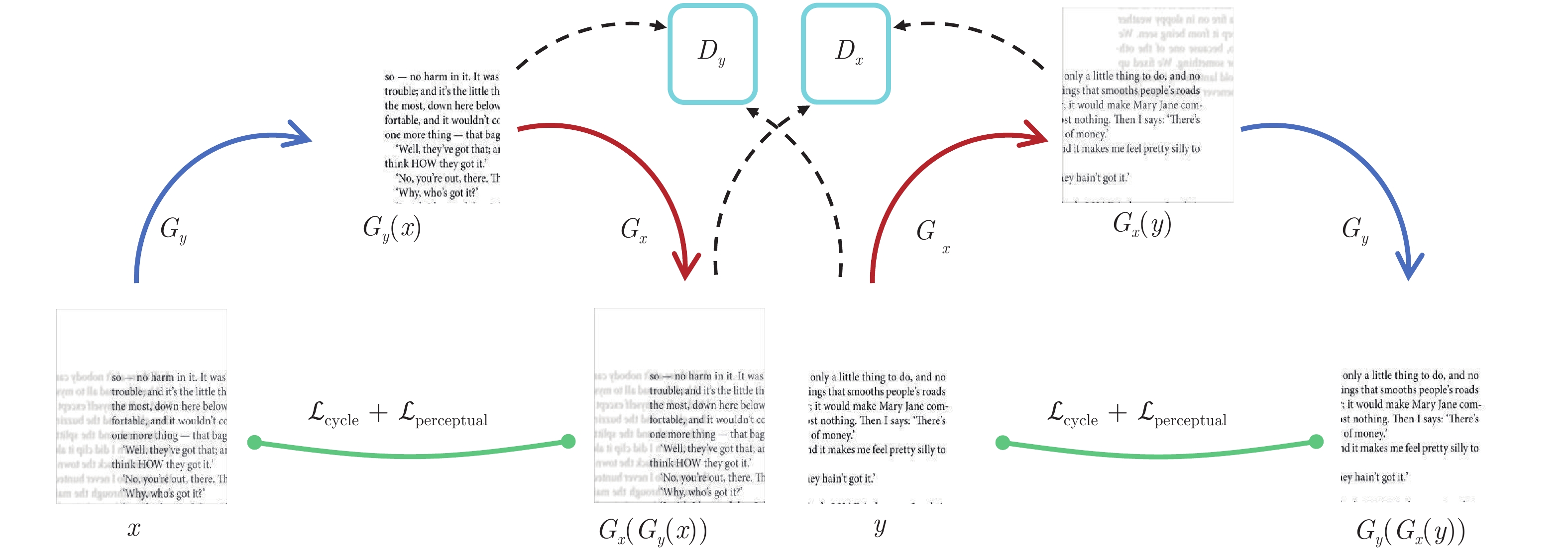
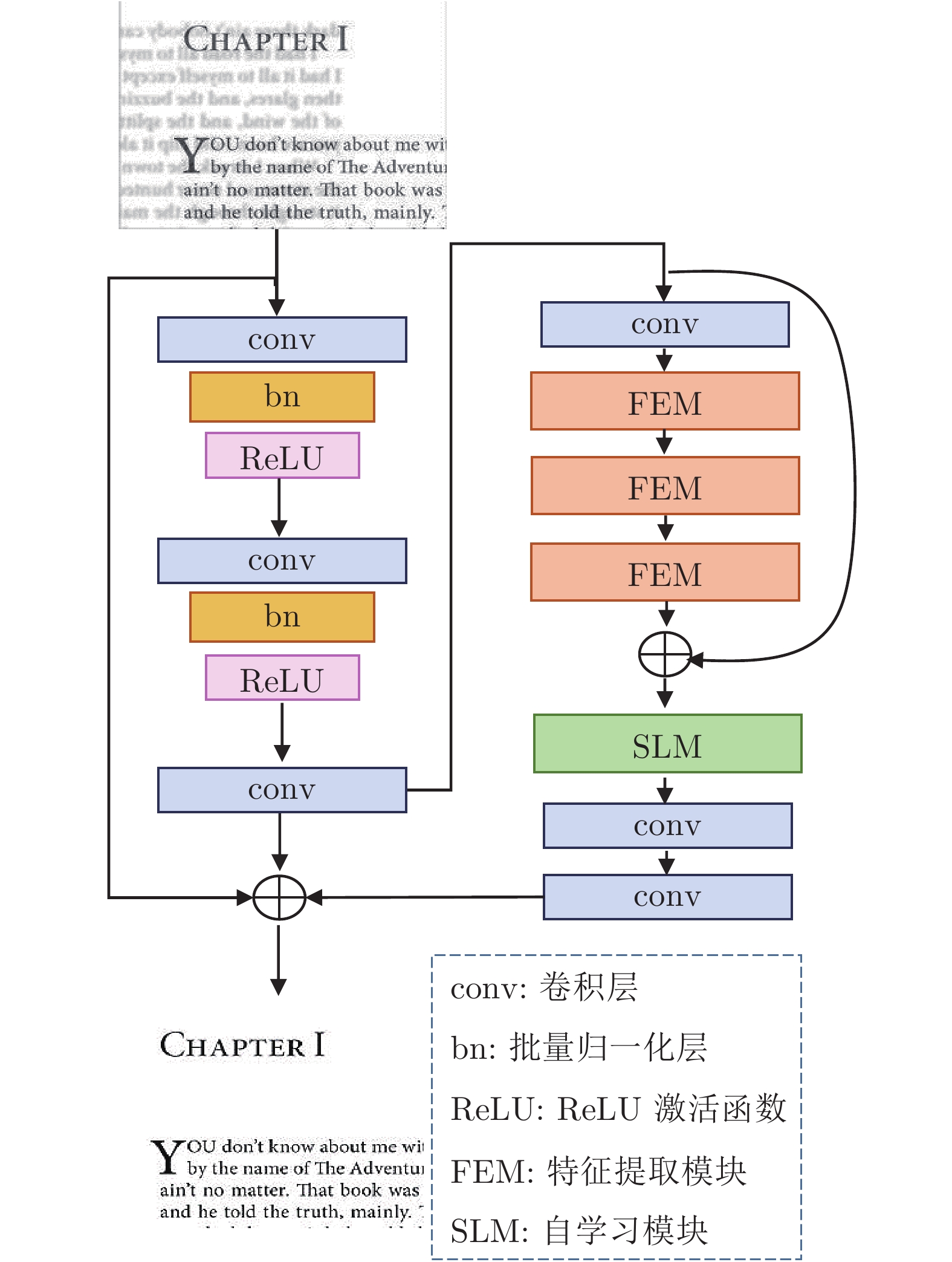
  • 图  1  S-CycleGAN的网络结构 (${G_y}$$G_x$表示生成器, $D_y$$D_x$表示判别器. $x$$y$分别表示输入的透射图像和无透射图像, ${\cal{L}}_{ {\rm{cycle}}}$${\cal{L}}_{ {\rm{perceptual}}}$分别表示循环一致性损失和感知损失)

    Fig.  1  Structure of S-CycleGAN ($G_y$ and $G_x$ are generators while $D_y$ and $D_x$ are discriminators, $x$ and $y$ represent the input bleed-through image and non-bleed-through image respectively, ${\cal{L}}_{ {\rm{cycle}}}$ and ${\cal{L}}_{ {\rm{perceptual}}}$ represent cycle consistency loss and perceptual loss respectively)
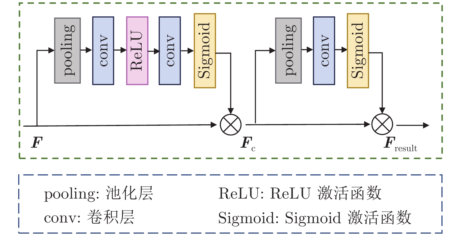
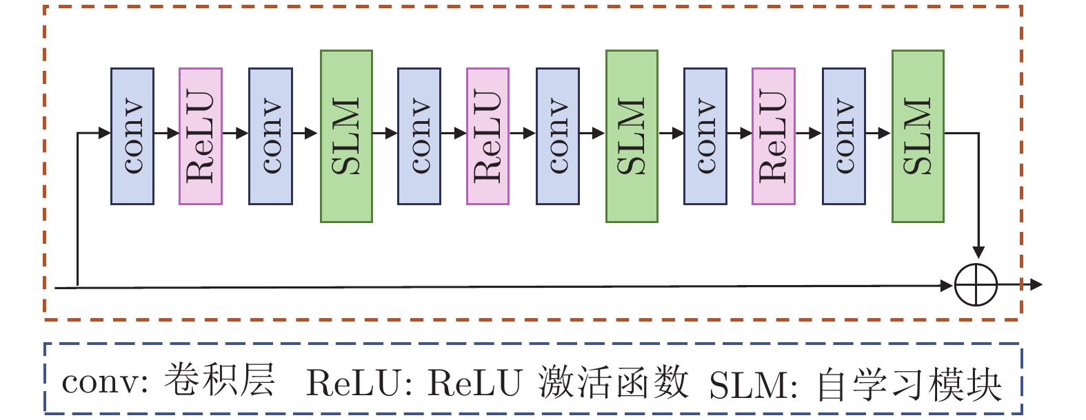
    图  2  生成器$G_y$的网络结构

    Fig.  2  The network structure of $G_y$

    图  3  FEM的网络结构

    Fig.  3  The network structure of FEM

    图  4  SLM的网络结构 ($F$表示自学习模块的输入, $F_ {\rm{c}}$表示自学习模块的中间输出, $F_{ {\rm{result}}}$表示自学习模块的输出)

    Fig.  4  The network structure of SLM ($F$ is the input to the self-learning module. $F_ {\rm{c}}$ is the intermediate output of the self-learning module. $F_{ {\rm{result}}}$ is the output of the self-learning module)

    图  5  自学习模块权重图

    Fig.  5  Self-learning module weight map

    图  6  判别器的网络结构

    Fig.  6  The network structure of discriminator

    图  7  不同权重系数$\omega$FMpFM评价指标的影响

    Fig.  7  Influence of different weight coefficient $\omega$ for FM and pFM

    图  8  各方法在DIBCO 2011数据集内一个样本的恢复结果

    Fig.  8  Experiment results of one sample in DIBCO 2011 datasets by different methods

    图  9  各方法在H-DIBCO 2016数据集的一个样本恢复结果

    Fig.  9  Experiment results of one sample in H-DIBCO 2016 datasets by different methods

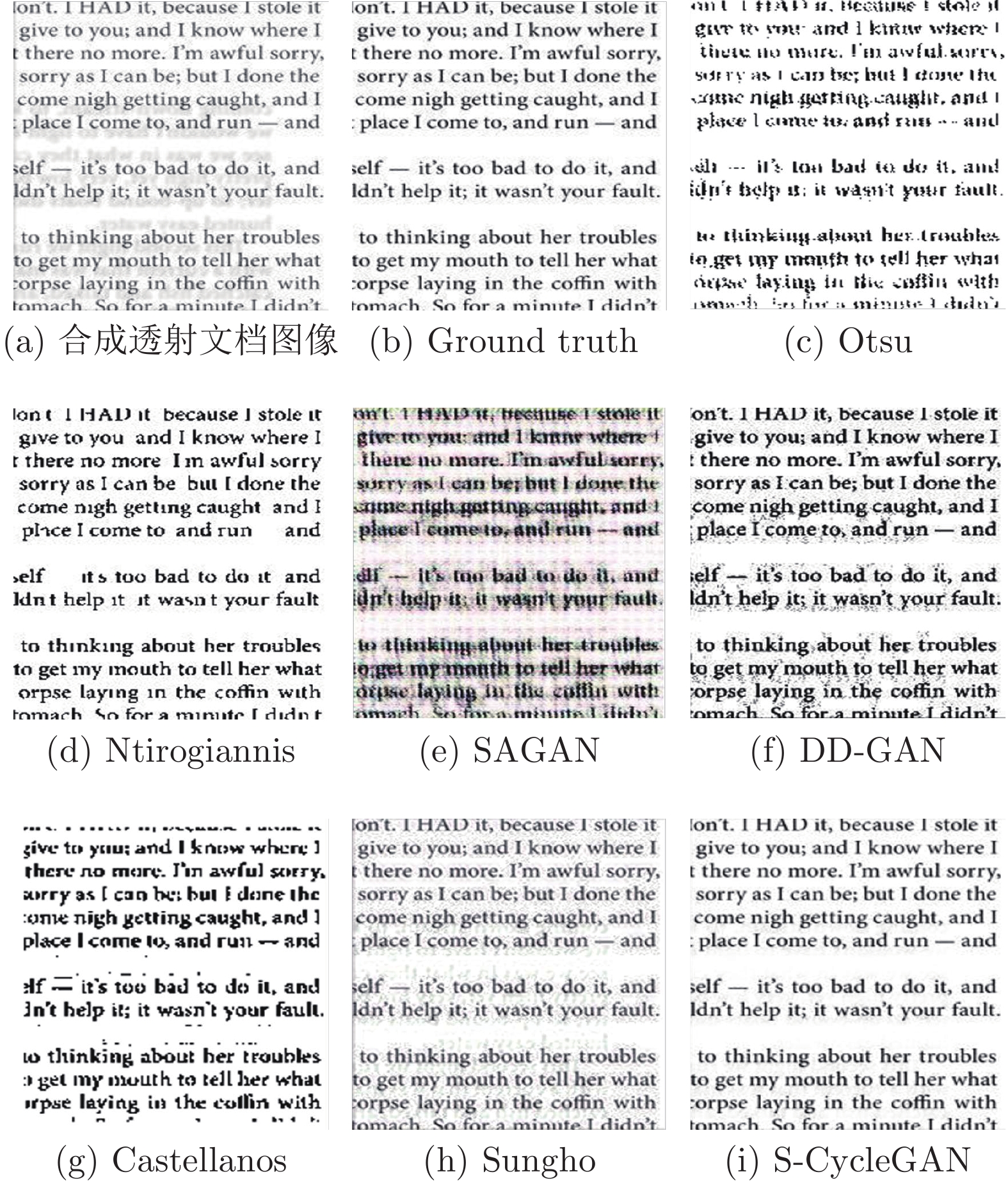
    图  10  各方法在合成数据集的一个样本恢复结果

    Fig.  10  Experiment results of one sample on synthetic document bleed-through datasets by different methods

    图  11  不同方法在全国大学英语六级试卷透射图像的恢复结果

    Fig.  11  Experiment results of CET-6 bleed-through datasets by different methods

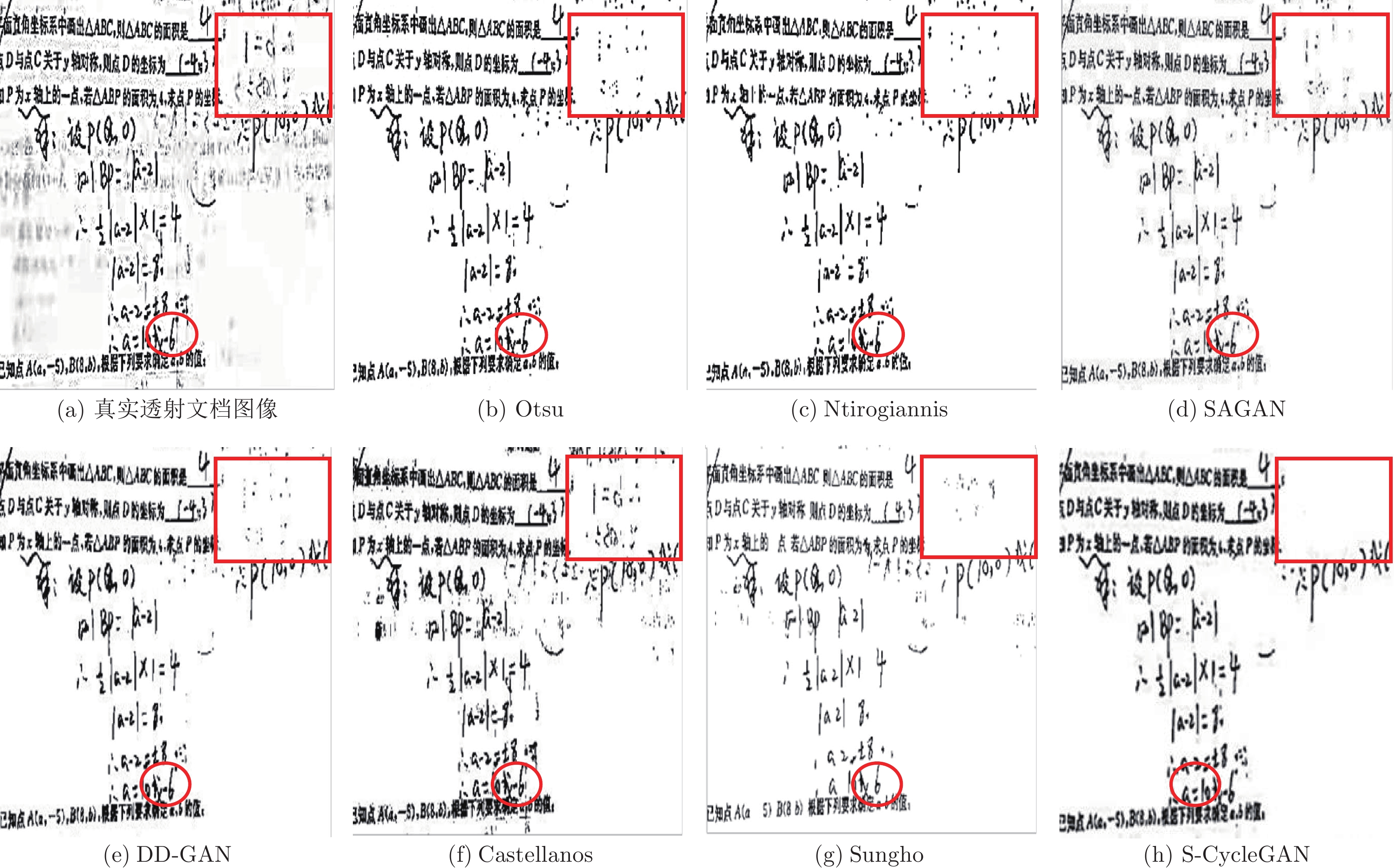
    图  12  不同方法在某初中数学试卷透射图像上的恢复结果

    Fig.  12  Experiment results of test papers bleed-through datasets by different methods

    图  13  不同网络结构在合成数据集上的消融实验

    Fig.  13  Ablation experiments of different network structures on synthetic datasets

    表  1  DIBCO数据集的文档透射图像恢复定量评价

    Table  1  Quantitative evaluation of document bleed-through image restoration of DIBCO datasets

    数据集 方法 PSNR (dB) FM (%) pFM (%) DRD
    Otsu 18.52 67.81 74.08 17.45
    Ntirogiannis 16.34 85.34 86.06 8.18
    SAGAN 21.55 87.47 92.28 5.97
    DIBCO DD-GAN 22.67 88.90 91.19 5.53
    2011 Castellanos 22.95 89.40 91.78 5.62
    Sungho 23.54 89.67 91.03 5.59
    S-CycleGAN 24.36 89.71 91.62 5.49
    Otsu 14.90 72.57 73.51 23.67
    Ntirogiannis 14.30 84.60 88.40 6.34
    SAGAN 19.64 89.75 90.85 6.35
    DIBCO DD-GAN 21.14 92.53 92.59 4.86
    2009 Castellanos 21.95 90.00 91.68 6.03
    Sungho 22.56 87.73 92.09 5.35
    S-CycleGAN 22.83 90.98 92.65 4.54
    Otsu 15.52 70.44 73.03 20.45
    Ntirogiannis 18.14 83.72 87.49 10.98
    SAGAN 20.35 91.64 92.71 5.64
    DIBCO DD-GAN 21.54 90.48 93.63 3.17
    2016 Castellanos 22.30 91.13 92.28 3.05
    Sungho 21.96 90.27 92.69 2.63
    S-CycleGAN 22.35 91.90 93.79 3.53
    下载: 导出CSV

    表  2  合成数据集的文档透射图像恢复定量评价

    Table  2  Quantitative evaluation of document bleed-through image restoration of synthetic datasets

    数据集 方法 PSNR (dB) FM (%) pFM (%) DRD
    Otsu 16.35 88.37 89.59 4.94
    Ntirogiannis 19.30 89.21 90.68 8.87
    SAGAN 16.05 87.61 91.28 5.21
    合成数据集 DD-GAN 20.45 90.51 90.01 4.73
    Castellanos 19.95 90.65 93.78 4.06
    Sungho 21.03 90.53 92.67 3.86
    S-CycleGAN 22.66 92.99 95.10 2.93
    下载: 导出CSV

    表  3  S-CycleGAN模块有效性客观评价指标对比

    Table  3  Objective evaluation indexes comparison for the modules in S-CycleGAN

    数据集 方法 PSNR (dB) FM (%) pFM (%) DRD
    CycleGAN 12.48 62.42 65.51 20.95
    合成数据集 无SLM 19.75 88.80 92.50 3.95
    S-CycleGAN 22.66 92.99 95.10 2.93
    CycleGAN 11.41 69.71 71.33 16.31
    H-DIBCO 无SLM 18.21 86.60 88.80 4.36
    2016 S-CycleGAN 22.35 91.90 93.79 3.53
    下载: 导出CSV
  • [1] Rasyidi H, Khan S. Historical document image binarization via style augmentation and atrous convolutions. Neural Computing and Applications, 2020, 33: 7339-7352
    [2] Gupta N, Goyal N. Machine learning tensor flow based platform for recognition of hand written text. In: Proceedings of the International Conference on Computer Communication and Informatics. Coimbatore, India: IEEE, 2021. 1−6
    [3] Han Y H, Wang W L, Liu H M, Wang Y Q. A combined approach for the binarization of historical tibetan document images. International Journal of Pattern Recognition and Artificial Intelligence, 2019, 33(14): 1954038. doi: 10.1142/S0218001419540387
    [4] Otsu N. A threshold selection method from gray-level histograms. IEEE Transactions on Systems Man Cybernetics-Systems, 2007, 9(1): 62-66
    [5] Ntirogiannis K, Gatos B, Pratikakis I. Performance evaluation methodology for historical document image binarization. IEEE Transactions on Image Processing, 2013, 22(2): 595-609 doi: 10.1109/TIP.2012.2219550
    [6] Su B, Lu S, Tan C L. Binarization of historical document images using the local maximum and minimum. In: Proceedings of the International Work-shop on Document Analysis Systems. Boston, USA: Work-shop on Document Analysis Systems, 2010. 154−160
    [7] Tensmeyer C, Martinez T. Document image binarization with fully convolutional neural networks. In: Proceedings of the International Conference on Document Analysis and Recognition. Kyoto, Japan: IEEE, 2017. 99−104
    [8] Wu Y, Rawls S, Abdalmageed W, Natarajan P. Learning document image binarization from data. In: Proceedings of the IEEE International Conference on Image Processing. Phoenix, USA: IEEE, 2016. 3763−3767
    [9] He S, Schomaker L. Deepotsu: document enhancement and binarization using iterative deep learning. Pattern Recognition, 2019, 91: 379-390 doi: 10.1016/j.patcog.2019.01.025
    [10] Kang S, Iwana B K, Uchida S. Complex image processing with less data-document image binarization by integrating multiple pre-trained u-net modules. Pattern Recognition, 2020, 109: 107577
    [11] Mondal R, Chakraborty D, Chanda B. Learning 2d morphological network for old document image binarization. In: Proceedings of the International Conference on Document Analysis and Recognition. Sydney, Australia: IEEE, 2019. 65−70
    [12] Goodfellow I J, Pouget-Abadie J, Mirza M, et al. Generative adversarial networks. Advances in Neural Information Processing Systems, 2014, 3: 2672-2680
    [13] Reed S, Akata Z, Mohan S, Tenka S, Schiele B, Lee H. Learning what and where to draw. In: Proceedings of the Neural Information Processing Systems. Barcelona, Spain: Curran Associates, 2016. 217−225
    [14] Konwer A, Bhunia A K, Bhowmick A, et al. Staff line removal using generative adversarial networks. In: Proceedings of the International Conference on Pattern Recognition. Beijing, China: IEEE, 2018. 1103−1108
    [15] De R, Chakraborty A, Sarkar R. Document image binarization using dual discriminator generative adversarial networks. IEEE Signal Processing Letters, 2020, 27: 1090-1094 doi: 10.1109/LSP.2020.3003828
    [16] Castellanos F J, Gallego A J, Jorge C Z. Unsupervised neural domain adaptation for document image binarization. Pattern Recognition, 2020, 119: 108099
    [17] Zhu J Y, Park T, Isola P. Unpaired image-to-image translation using cycle-consistent adversarial networks. In: Proceedings of the IEEE International Conference on Computer Vision. Venice, Italy: IEEE, 2017. 2223−2232
    [18] Sajjadi M, Scholkopf B, Hirsch M. EnhanceNet: single image super-resolution through automated texture synthesis. In: Proceedings of the IEEE International Conference on Computer Vision. Venice, Italy: IEEE, 2017. 4501−4510
    [19] Simonyan K, Zisserman A. Very deep convolutional networks for large-scale image recognition. In: Proceedings of the International Conference on Learning Representations. California, USA, 2015. 1−14
    [20] Jia D, Dong W, Socher R, Li L J, Kai L, Li F F. Imagenet: A large-scale hierarchical image database. In: Proceedings of the IEEE Conference on Computer Vision and Pattern Recognition. Miami, USA: IEEE, 2009. 248−255
    [21] Pratikakis I, Gatos B, Ntirogiannis K. Icdar 2013 document image binarization contest. In: Proceedings of the International Conference on Document Analysis and Recognition. Washington, USA: IEEE, 2013. 1471−1476
    [22] Pratikakis I, Gatos B, Ntirogiannis K. Icfhr 2012 competition on handwritten document image binarization. In: Proceedings of the International Conference on Frontiers in Handwriting Recognition. Bari, Italy: IEEE, 2012. 817−822
    [23] Ntirogiannis K, Gatos B, Pratikakis I. Icfhr 2014 competition on handwritten document image binarization. In: Proceedings of the International Conference on Frontiers in Handwriting Recognition. Hersonissos, Greece: IEEE, 2014. 809−813
    [24] Pratikakis I, Zagoris K, Barlas G, Gatos B. Icdar2017 competition on document image binarization. In: Proceedings of the International Conference on Document Analysis and Recognition. Kyoto, Japan: IEEE, 2017. 2379−2140
    [25] Pratikakis I, Gatos B, Ntirogiannis K. Icdar 2011 document image binarization contest. In: Proceedings of the International Conference on Document Analysis and Recognition. Beijing, China: IEEE, 2011. 1506−1510
    [26] Gatos B, Ntirogiannis K, Pratikakis I. Icdar 2009 document image binarization contest. In: Proceedings of the International Conference on Document Analysis and Recognition. Barcelona, Spain: IEEE, 2009. 1375−1382
    [27] Pratikakis I, Zagoris K, Barlas G, Gatos B. Icfhr 2016 Handwritten document image binarization contest. In: Proceedings of the International Conference on Frontiers in Handwriting Recognition. Shenzhen, China: IEEE, 2016. 2167−6445
    [28] Zhang X, Goodfellow I, Metaxas D, Odena A. Self-attention generative adversarial networks. In: Proceedings of the International Conference on Machine Learning. California, USA, 2019. 7354−7363
    [29] Suh S, Kim J, Lukowicz P, Lee Y O. Two-stage generative adversarial networks for document image binarization with color noise and background removal. 2020, arXiv: 2010.10103
  • 加载中
图(13) / 表(3)
计量
  • 文章访问数:  1018
  • HTML全文浏览量:  158
  • PDF下载量:  255
  • 被引次数: 0
出版历程
  • 收稿日期:  2022-03-10
  • 录用日期:  2022-07-21
  • 网络出版日期:  2022-09-13
  • 刊出日期:  2023-01-07

目录

/

返回文章
返回