2.845

2023影响因子

(CJCR)

  • 中文核心
  • EI
  • 中国科技核心
  • Scopus
  • CSCD
  • 英国科学文摘

留言板

尊敬的读者、作者、审稿人, 关于本刊的投稿、审稿、编辑和出版的任何问题, 您可以本页添加留言。我们将尽快给您答复。谢谢您的支持!

姓名
邮箱
手机号码
标题
留言内容
验证码

多率量测下随机跳变系统迁移交互多模型估计

高爽 栾小丽 赵顺毅 刘飞

欧阳慧珉, 王健, 张广明, 梅磊, 邓歆. 基于新型滑模算法的双摆旋转起重机消摆跟踪控制. 自动化学报, 2019, 45(7): 1344-1353. doi: 10.16383/j.aas.c180452
引用本文: 高爽, 栾小丽, 赵顺毅, 刘飞. 多率量测下随机跳变系统迁移交互多模型估计. 自动化学报, 2023, 49(1): 210−218 doi: 10.16383/j.aas.c220011
OUYANG Hui-Min, WANG Jian, ZHANG Guang-Ming, MEI Lei, DENG Xin. Tracking and Anti-sway Control for Double-pendulum Rotary Cranes Using Novel Sliding Mode Algorithm. ACTA AUTOMATICA SINICA, 2019, 45(7): 1344-1353. doi: 10.16383/j.aas.c180452
Citation: Gao Shuang, Luan Xiao-Li, Zhao Shun-Yi, Liu Fei. Transfer interacting multiple model state estimator for Markovian jump linear systems with multi-rate measurements. Acta Automatica Sinica, 2023, 49(1): 210−218 doi: 10.16383/j.aas.c220011

多率量测下随机跳变系统迁移交互多模型估计

doi: 10.16383/j.aas.c220011
基金项目: 国家自然科学基金(61991402, 61833007, 61991400), 江苏省研究生科研与实践创新计划(KYCX21-2007) 资助
详细信息
    作者简介:

    高爽:江南大学博士研究生. 2018年获得江南大学学士学位. 主要研究方向为状态估计, 贝叶斯估计理论. E-mail: gaoshuang@stu.jiangnan.edu.cn

    栾小丽:江南大学教授. 2010年获得江南大学博士学位. 主要研究方向为复杂工业过程建模、控制与优化. 本文通信作者. E-mail: xlluan@jiangnan.edu.cn

    赵顺毅:江南大学研究员. 2015年获得江南大学博士学位. 主要研究方向为随机信号处理, 贝叶斯估计理论和故障检测与诊断. E-mail: shunyi.s.y@gmail.com

    刘飞:江南大学教授. 2002年获得浙江大学博士学位. 主要研究方向为过程控制, 过程系统工程. E-mail: fliu@jiangnan.edu.cn

Transfer Interacting Multiple Model State Estimator for Markovian Jump Linear Systems With Multi-rate Measurements

Funds: Supported by National Natural Science Foundation of China (61991402, 61833007, 61991400) and the Postgraduate Research Practice Innovation Program of Jiangsu Province (KYCX21-2007)
More Information
    Author Bio:

    GAO Shuang Ph.D. candidate at Jiangnan University. She received her bachelor degree from Jiangnan University in 2018. Her research interest covers state estimation and Bayesian estimation theory

    LUAN Xiao-Li Professor at Jiangnan University. She received her Ph.D. degree from Jiangnan University in 2010. Her main research interest is modeling, control and optimization of complex industrial process. Corresponding author of this paper

    ZHAO Shun-Yi Researcher at Jiangnan University. He received his Ph.D. degree from Jiangnan University in 2015. His research interest covers statistical signal processing, Bayesian estimation theory, and fault detection and diagnosis

    LIU Fei Professor at Jiangnan University. He received his Ph.D. degree from Zhejiang University in 2002. His research interest covers process control and process system engineering

  • 摘要: 实际工业过程中, 量测数据除了在线仪表采集的快速率数据, 还有离线化验等慢速率辅助量测数据. 为了更好地利用离线化验数据, 增加在线估计的精度, 针对随机跳变系统, 引入迁移学习思想, 提出迁移交互多模型估计 (Transfer interacting multiple model state estimator, IMM-TF) 新策略. 首先, 将离线化验数据的边缘分布作为可以迁移的知识, 迁移到贝叶斯后验分布, 实现辅助量测数据的充分利用. 其次, 利用KL (Kullback-Leibler) 散度度量知识迁移前后任务间的差异性, 求解最优的贝叶斯迁移估计器. 同时, 结合慢速率量测, 利用平滑策略获取待迁移的估计值, 解决多率量测下的迁移估计难题. 然后, 利用影响力函数构建辅助量测数据与估计性能之间的解析关系, 从而对迁移效果进行定量评价. 最后, 通过在目标跟踪实例中的应用, 表明所提方法的有效性及优越性.
  • 旋转起重机作为常见的起重机械, 由于其结构简单、占用空间小、无需大型行走设备等优点, 因此被广泛地应用于建筑工地、矿山、港口等场合.然而, 旋臂的加减速会使负载产生摆动, 不仅降低了生产效率, 而且会损坏货物, 造成人员伤亡等.针对该问题, 已经有学者作了大量的研究, 并且提出了许多有效的方法[1-19].但是, 当负载形状不规则或者吊钩的质量不能忽视时, 该摆动会呈现出更加复杂的两级摆动现象.该现象极大地增加了系统特性分析和控制器设计的难度, 因此如何设计出可以有效抑制两级摆动的控制算法问题已经成为学术界和产业界研究的难点和热点.

    近年来, 已经有学者针对起重机系统双摆抑制问题展开了一些研究[20-35]. Tang等针对2-D双摆桥式起重机系统中由于台车运动和外部风干扰而引起的荷载摆动, 提出了结合两种运动轨迹的方法, 即其中一个轨迹用来抑制台车运动引起的摆动, 另一个轨迹用来抑制风干扰引起的摆动, 仿真与实验验证了该方法的有效性[20].陈鹤等针对双摆桥式吊车系统提出了一种时间最优轨迹规划方法, 该方法在构造以时间为代价函数的基础上, 将优化问题转化成非线性规划问题, 通过仿真与实验验证了该方法的有效性[21]. Zhang等针对双摆桥式起重机在线规划了一条台车轨道, 该轨道由两部分组成分别实现双摆抑制和台车定位, 仿真验证了该轨道对于参数变化和外部干扰具有鲁棒性[22]. Huang等针对2-D双摆桥式起重机系统提出了一种新型指令整形方法, 仿真与实验验证了该方法的有效性[23].孙宁等针对双摆桥式吊车系统提出了一种基于轨迹规划的消摆定位控制方法, 该方法在充分考虑系统安全性(摆动幅值)等物理约束基础上, 通过构造新颖的平坦输出信号, 将施加在台车运动和两级摆动上的约束/指标转化为对平坦输出的约束, 从而将轨迹规划转化为凸优化问题, 通过数值仿真验证了该方法的有效性[24]. Masoud等针对双摆桥式起重机系统提出了一种频率调制输入整形方法, 该方法是由一个基于闭环系统的第一阶摆动频率的输入整形器和一个虚拟反馈控制环节构成, 仿真与实验验证了该方法的有效性[25]. Maleki等针对双摆旋转起重机系统中存在两级摆动模态的问题, 提出了一种两级模态特定不敏感输入整形器, 通过与两级模态零摆动输入整形器的比较验证了该方法的有效性, 同时也证明了其对旋臂旋转角速度与角加速度变化具有鲁棒性[26]. Masoud等针对双摆桥式起重机系统将输入整形法和闭环控制法相结合, 具体而言, 首先基于假设的双摆系统第一阶模态设计基础整形器, 再设计一个虚拟的带有积分器反馈控制器消除由第一阶模态引起的残留摆动, 通过仿真与实验验证了该方法的有效性[27]. Manning等针对2-D双摆桥式起重机系统设计了一个SI2M (Two-mode specified-insensitivity)输入整形器, 并通过与ZV2M (Two-mode zero vibration)输入整形器比较验证了所提方法对于绳长变化更具有鲁棒性[28]. Sung等针对2-D双摆桥式起重机系统中应用输入整形技术进行消摆控制时关于参数变化的鲁棒性问题, 通过比较仿真和实验指出SI2M整形器性能最好[29]. Qian等针对双摆桥式起重机消摆控制问题, 提出了一种基于SIRMs (Single-input-rule modules)的模糊控制器, 比较仿真验证了该方法的有效性[30]. Ouyang等提出了一种基于LMI (Linear matrix inequality)的简易鲁棒控制器解决双摆桥式起重机消摆控制问题[31]. Zhang等考虑了起重机系统中参数不确定性等对控制性能的影响, 提出了一个自适应控制器, 系统稳定性通过李雅普诺夫定理和芭芭拉特引理进行分析, 仿真结果验证了其有效性[32]. Tuan等针对双摆桥式起重机消摆控制问题, 提出了一个传统滑模控制器和一个多层滑模控制器, 仿真结果验证了其有效性[33]. Sun等针对双摆桥式起重机消摆控制问题, 提出了一种饱和非线性输出反馈控制器和一种非线性准PID控制, 实验结果验证了其有效性[34-35].开环控制方式[20-29], 即在设计控制器时不反馈摆角信息, 如轨迹规划法和基于输入整形技术已经应用于双摆桥式起重机系统.这些方法虽然具有控制器结构简单, 易于实现等优点, 但是它们过于依赖系统精确模型, 当系统受到外部干扰后控制性能会降低.另一方面, 虽然如文献[30-35]所提出的闭环控制方式可以为起重机系统提供鲁棒或自适应控制算法, 但是由于它们的系统阻尼比大都设定为常数.因此很难同时实现旋臂的高精度定位和两级摆角的抑制.为此, 本文将提出一种变阻尼的算法从而实现前述问题.进一步而言, 不同于2-D桥式起重机的平面摆动, 旋转起重机系统中的双摆均为圆锥摆, 系统特性更加复杂.据笔者所知, 到目前为止, 尚无针对双摆旋转起重机摆角抑制的相关报道.

    本文在建立双摆旋转起重机动力学模型的基础上, 采用干扰观测器将其解耦成两个独立的线性系统, 即起伏子系统和旋转子系统.其次, 基于此线性模型分别为其设计含有非线性滑模面的滑模控制器, 并通过李雅普诺夫定理分析其稳定性.最后比较仿真和定量分析验证本文所提方法的有效性.

    综上, 本文的主要创新之处可总结为如下几点:

    1) 据笔者所知, 首次将具有非线性滑模面的滑模控制器应用于双摆旋转起重机系统.

    2) 不同于传统的线性滑模面, 本文所提出的非线性滑模面可以为闭环系统提供一个可变的阻尼比, 从而在提高旋臂定位精度的同时实现对两级摆角的抑制.

    图 1所示旋转起重机模型中$M_{0}$, $m_{1}$和$m_{2}$分别表示旋臂质量、吊钩质量和负载质量; $L$, $l_{1}$和$l_{2}$分别表示旋臂长度、悬绳长度和吊绳长度; $\theta_{1}$和$\theta_{3}$分别表示吊钩摆角和负载摆角在旋臂起伏方向上的分量; $\theta_{2}$和$\theta_{4}$分别表示吊钩摆角和负载摆角在旋臂起伏方向上的分量; $\theta_{5}$和$\theta_{6}$则表示旋臂起伏角和旋转角.

    图 1  双摆旋转起重机模型
    Fig. 1  Dynamic model of double-pendulum rotary crane

    为了进一步分析和设计控制系统, 对旋转起重机做如下几点合理假设[1-3, 6-8, 28-31]:

    1) 吊钩和负载均看作质点, 悬绳和吊绳的拉力和质量忽略不计.

    2) 由于摆角$\theta_{i}~(i=1, 2, 3, 4)$在旋臂到达目标位置时较小, 因此$\cos\theta_{i}=1$, $\sin\theta_{i}=\theta_{i}$, $\dot\theta_{i}=0$, $\dot\theta_{i}^2=0$以及$\ddot\theta_{i}=0$等均成立.

    根据拉格朗日运动方程, 双摆旋转起重机系统动力学模型如下所示:

    $ \begin{align} (m_{1}+&m_{2})l_{1}^{2}(1+\theta_{1}^{2})\ddot\theta_{1}+(m_{1} +m_{2})l_{1}^{2}\theta_{1}\theta_{2}\ddot{\theta}_{2}+ \nonumber\\ &m_{2}l_{1}l_{2}(1+\theta_{1}\theta_{3})\ddot{\theta}_{3}+ m_{2}l_{1}l_{2}\theta_{1}\theta_{4}\ddot{\theta}_{4} + \nonumber\\ &(m_{1}+m_{2})l_{1}L(\cos\theta_{5}-\theta_{1}\sin\theta_{5})\ddot\theta_{5} -\nonumber\\ &\Big((m_{1}+m_{2})l_{1}^{2}\theta_{2}+m_{2}l_{1}l_{2}\theta_{4}\Big) \ddot\theta_{6}+\nonumber\\ &(m_{1}+m_{2})l_{1}^2\theta_{1}\dot\theta_{1}^2+m_{2}l_1l_2\theta_{1} \dot\theta_{3}^2+ \nonumber\\ &\Big((m_{1}+m_{2})l_{1}^2\theta_{1}\dot\theta_{2}-2(m_{1}+ m_{2})l_{1}^{2}\dot\theta_{6}\Big)\dot\theta_{2} +\nonumber\\ &(m_{2}l_{1}l_{2}\theta_{1}\dot\theta_{4}-2m_{2}l_1l_2\dot\theta_{6}) \dot\theta_{4}- \nonumber\\ &(m_1+m_2)l_1L(\sin\theta_{5}+\theta_1\cos\theta_{5})\dot\theta_{5}^2 -\nonumber\\ &\Big((m_1+m_2)l_1^2\theta_1+m_2l_1l_2\theta_3\Big)\dot\theta_6^2- \nonumber\\ &\Big((m_1+m_2)l_1L\sin\theta_5\Big)\dot\theta_6^2+\nonumber\\ &(m_1+m_2)l_1g\theta_1=0 \end{align} $

    (1)

    $ \begin{align} (m_{1}+&m_{2})l_{1}^{2}\theta_1\theta_2\ddot\theta_{1}+(m_{1}+ m_{2})l_{1}^{2}(1+\theta_{2}^2)\ddot{\theta}_{2}+ \nonumber\\ &m_{2}l_{1}l_{2}\theta_2\theta_3\ddot{\theta}_{3}+m_{2}l_{1}l_{2} (1+\theta_{2}\theta_{4})\ddot{\theta}_{4}- \nonumber\\ &(m_{1}+m_{2})l_{1}L\theta_2\sin\theta_5\ddot\theta_{5}+ (m_{1}+m_{2})l_{1}^{2}\theta_{1}\ddot\theta_{6} +\nonumber\\ &\Big((m_{1}+m_{2})l_1L\sin\theta_5+m_{2}l_{1}l_{2}\theta_{3}\Big)\ddot\theta_{6}+ \nonumber\\ &\left((m_{1}+m_{2})l_{1}^2\theta_{2}\dot\theta_{1}+2(m_1+m_2)l_1^2\dot\theta_6\right)\dot\theta_1 + \nonumber\\ &(m_1+m_2)l_1^2\theta_2\dot\theta_{2}^2+m_2l_1l_2\theta_2\dot\theta_{4}^2+ \nonumber\\ &(m_2l_1l_2\theta_2\dot\theta_3+2m_2l_1l_2\dot\theta_6)\dot\theta_{3}+ \nonumber\\ &\left((m_1+m_2)l_1L\cos\theta_5(2\dot\theta_6-\theta_2\dot\theta_5)\right)\dot\theta_5- \nonumber\\ &\Big((m_1+m_2)l_1^2\theta_2+m_2l_1l_2\theta_4\Big)\dot\theta_6^2 +\nonumber\\ &(m_1+m_2)l_1g\theta_2=0 \end{align} $

    (2)

    $ \begin{align} m_2l_1l_2&(1+\theta_1\theta_3)\ddot\theta_1+m_2l_1l_2\theta_2\theta_3\ddot\theta_2 +\nonumber\\ &m_2l_2^2(1+\theta_3^2)\ddot\theta_3+m_2l_2^2\theta_3\theta_4\ddot\theta_4 +\nonumber\\ &m_2l_2L(\cos\theta_5-\theta_3\sin\theta_5)\ddot\theta_5 -\nonumber\\ &(m_2l_2^2\theta_4+m_2l_1l_2\theta_2)\ddot\theta_6+ m_2l_1l_2\theta_3\dot\theta_1^2 +\nonumber\\ &(m_2l_1l_2\theta_3\dot\theta_2-2m_2l_1l_2\dot\theta_6)\dot\theta_2+m_2l_2^2\theta_3\dot\theta_3^2 +\nonumber\\ &(m_2l_2^2\theta_3\dot\theta_4-2m_2l_2^2\dot\theta_6)\dot\theta_4 -\nonumber\\ &m_2l_2L(\sin\theta_5+\theta_3\cos\theta_5)\dot\theta_5^2 -\nonumber\\ &(m_2l_2^2\theta_3+m_2l_1l_2\theta_1+m_2l_2L\sin\theta_5)\dot\theta_6^2 +\nonumber\\ &m_2l_2g\theta_3=0\end{align} $

    (3)

    $ \begin{align} m_2l_1l_2&\theta_1\theta_4\ddot\theta_1+m_2l_1l_2(1+\theta_2 \theta_4)\ddot\theta_2 +m_2l_2^2\theta_3\theta_4\ddot\theta_3+\nonumber\\ &m_2l_2^2(1+\theta_4^2)\ddot\theta_4-m_2l_2L\theta_4\sin\theta_5\ddot\theta_5 +\nonumber\\ &(m_2l_2^2\theta_3+m_2l_2L\sin\theta_5+m_2l_1l_2\theta_1)\ddot\theta_6 +\nonumber\\ &(m_2l_1l_2\theta_4\dot\theta_1+2m_2l_1l_2\dot\theta_6)\dot\theta_1+m_2l_1l_2\theta_4\dot\theta_2^2 +\nonumber\\ &(m_2l_2^2\theta_4\dot\theta_3+2m_2l_2^2\dot\theta_6)\dot\theta_3+m_2l_2^2\theta_4\dot\theta_4^2 +\nonumber\\ &(2m_2l_2L\cos\theta_5\dot\theta_6-m_2l_2L\theta_4\cos\theta_5\dot\theta_5)\dot\theta_5 - \nonumber\\ &(m_2l_1l_2\theta_2+m_2l_2^2\theta_4)\dot\theta_6^2+m_2l_2g\theta_4=0 \end{align} $

    (4)

    $ J_{k+4}\ddot{\theta}_{k+4}+d_{k+4}=\gamma_{k+4}, k=1, 2 $

    (5)

    其中, $g$, $\dot\theta_{i}$, $\ddot\theta_{i}~(i=1, 2, 3, 4, 5, 6), $ $J_{k+4}$, $d_{k+4}$和$\gamma_{k+4}$分别表示重力加速度、起伏方向和旋转方向的摆角角速度, 起伏和旋转角速度及其对应的角加速度, 起伏和旋转方向的转动惯量, 包括了摩擦项和其他被忽略的非线性项的系统外界干扰以及各电机的驱动力矩.

    为了方便设计控制器, 采用了如图 2所示的干扰观测器(Disturbance observer, DOB)[11, 17, 36-40].

    图 2  含有干扰观测器的控制系统
    Fig. 2  Control system with a disturbance observer

    图 2中$\hat{d}_{k+4}$和$\omega_{k+4}$分别为干扰项的观测值和低通滤波器的截止频率.为了获得良好的控制性能, 该参数由试凑法可得$\omega_{k+4}=40 \rm Hz$.笔者已经验证了其在低频域可对干扰项$d_{k+4}$进行很好的补偿[11].因此, 可得:

    $ \begin{align} \ddot{\theta}_{i+4}=v_{k+4}, \hspace{0.2cm}k=1, 2 \end{align} $

    (6)

    式中, $v_{k+4}$表示起伏子系统和旋转子系统的控制输入.

    根据前述假设, 结合式(1)~(4)和式(6), 可得,

    $ (m_1+m_2)l_1^2\ddot\theta_1+m_2l_1l_2\ddot\theta_3+(m_1+m_2)\times \nonumber \\ \qquad l_1L\cos\theta_{5f}\ddot\theta_5=-(m_1+m_2)l_1g\theta_1 $

    (7)

    $ m_2l_1l_2\ddot\theta_1+m_2l_2^2\ddot\theta_3+m_2l_2 \times \nonumber \\ \qquad L\cos\theta_{5f}\ddot{\theta}_5=-m_2l_2g\theta_3 $

    (8)

    $ \ddot\theta_5=v_5 $

    (9)

    $(m_1+m_2)l_1^2\ddot\theta_2+m_2l_1l_2\ddot\theta_4+(m_1+m_2)\times \nonumber \\ \qquad l_1L\sin\theta_{5f}\ddot\theta_6=-(m_1+m_2)l_1g\theta_2 $

    (10)

    $ m_2l_1l_2\ddot\theta_2+m_2l_2^2\ddot\theta_4+m_2l_2\times \nonumber \\ \qquad L\sin\theta_{5f}\ddot{\theta}_6=-m_2l_2g\theta_4 $

    (11)

    $ \ddot\theta_6=v_6 $

    (12)

    其中, $\theta_{5f}$为起伏角的目标值.

    式(7)~(12)写成矩阵形式可得,

    $ M_1\ddot{z}_1+G_1z_1=v_5 $

    (13)

    $ \begin{align} &M_{1}=\left[ \begin{array}{ccccccc} 1 & \dfrac{m_2l_2}{(m_1+m_2)l_1} & \dfrac{L\cos\theta_{5f}}{l_1} \\ \dfrac{l_1}{l_2} & 1 & \dfrac{L\cos\theta_{5f}}{l_2} \\ 0 & 0 & 1 \\ \end{array} \right] \nonumber \\ &G_1=\left[ \begin{array}{ccccccc} \dfrac{g}{l_1} & 0 & 0 \\ 0 & \dfrac{g}{l_2} & 0 \\ 0 & 0 & 0 \\ \end{array} \right] \nonumber \\ &\ddot{z}_{1}=\left[ \begin{array}{cccccc} \ddot{\theta}_{1} & \ddot{\theta}_{3} & \ddot{\theta}_{5} \\ \end{array} \right]^{\rm T}, z_{1}=\left[ \begin{array}{cccccc} \theta_{1} & \theta_{3} & \theta_{5} \\ \end{array} \right]^{\rm T} \nonumber \end{align} $

    (14)

    $ \begin{align} &M_2\ddot{z}_2+G_2z_2=v_6 \\ &M_{2}=\left[ \begin{array}{ccccccc} 1 & \dfrac{m_2l_2}{(m_1+m_2)l_1} & \dfrac{L\sin\theta_{5f}}{l_1} \\ \dfrac{l_1}{l_2} & 1 & \dfrac{L\sin\theta_{5f}}{l_2} \\ 0 & 0 & 1 \\ \end{array} \right], \nonumber \\ &G_2=\left[ \begin{array}{ccccccc} \dfrac{g}{l_1} & 0 & 0 \\ 0 & \dfrac{g}{l_2} & 0 \\ 0 & 0 & 0 \\ \end{array} \right] \nonumber \\ &\ddot{z}_{2}=\left[ \begin{array}{cccccc} \ddot{\theta}_{2} & \ddot{\theta}_{4} & \ddot{\theta}_{6} \\ \end{array} \right]^{\rm T}, z_{2}=\left[ \begin{array}{cccccc} \theta_{2} & \theta_{4} & \theta_{6} \\ \end{array} \right]^{\rm T} \nonumber \end{align} $

    由式(13)和式(14)可知, 起伏子系统和旋转子系统拥有非常相似的结构, 因此本文可以为其设计相似的控制器.

    本节将为双摆旋转起重机设计一种新型含有非线性滑模面的滑模控制器从而同时实现旋臂高精度跟踪和摆角抑制.不同于传统的线性滑模面, 本节所提出的非线性滑模面可以使闭环系统的阻尼比从最初的较小值变化为最终的较大值.较小的阻尼比可以为系统提供较快的响应速度而较大的阻尼比则可减小超调量从而使得旋臂更加精确地跟踪给定轨迹.

    基于式(13)和式(14)所示起重机线性模型, 本文所提出的非线性滑模面如下所示:

    $ \begin{align} &S_k=(\Gamma_k-\Phi_kP_k)e_{1k}+\dot{e}_{1k}, \hspace{0.2cm}k=1, 2 \\ &e_{1k}=\left[ \begin{array}{cccc} \theta_{k} \\ \theta_{k+2} \\ \theta_{k+4}-\theta_{(k+4)d} \\ \end{array} \right] \nonumber \\ &\dot{e}_{1k}=\left[ \begin{array}{cccc} \dot{\theta}_{k} \\ \dot{\theta}_{k+2} \\ \dot{\theta}_{k+4}-\dot{\theta}_{(k+4)d} \\ \end{array} \right] \nonumber \end{align} $

    (15)

    其中, $\theta_{(k+4)d}$和$\dot{\theta}_{(k+4)d}$分别表示旋臂起伏角和旋转角的目标位移轨迹和目标速度轨迹. $P_k$是正定矩阵并满足如下所示的李雅普诺夫方程:

    $ \begin{align} P_k\Gamma_k^{\rm T}+\Gamma_kP_k=-W_k, \hspace{0.2cm}k=1, 2 \end{align} $

    (16)

    其中, $W_k$也是正定矩阵.选取合适的满秩矩阵$\Gamma_k$使得其满足赫尔维茨定理并为闭环系统提供一个较小的初始阻尼比.非线性函数$\Phi_k$则要根据系统的输出(即, 旋臂的起伏角、旋转角以及各方向第一、二级摆角)进行选择并可用来调节闭环系统的阻尼比.虽然该函数的选取并不唯一, 但是必须满足以下两个性质:

    1) 必须对于系统输出可微并保证滑动模态存在.

    2) 必须从$0$变化成一个负值.

    因此, 本文采用如下所示的非线性函数进行控制器的设计[36]

    $ \begin{align} &\Phi_k=\left[ \begin{array}{cccc} \phi_1 & 0 & 0 \\ 0 & \phi_2 & 0 \\ 0 & 0 & \phi_3 \\ \end{array} \right] \\ &\phi_1=-\lambda_{1k}{\rm e}^{-\theta_{k}^{2}}, \phi_2=-\lambda_{2k}{\rm e}^{-\theta_{k+2}^{2}} \nonumber \\ &\phi_3=-\lambda_{3k}{\rm e}^{-(\theta_{k+4}-\theta_{(k+4)d})^{2}} \nonumber \end{align} $

    (17)

    式中, $\lambda_{ik}$ ($i=1, 2, 3, k=1, 2$)为正值, 而$e^{(\cdot)}$表示指数函数.

    通过设计合适的控制律, 系统的所有状态量都可以进入预期的滑模面上.当处于滑模面时, 即$S_k=0$, 可得:

    $ \begin{align} (\Gamma_k-\Phi_kP_k)e_{1k}+\dot{e}_{1k}=0 \end{align} $

    (18)

    进一步整理可得:

    $ \begin{align} \dot{e}_{1k}= &-\Gamma_ke_{1k}+\Phi_kP_ke_{1k} =\nonumber\\ &(-\Gamma_k+\Phi_kP_k)e_{1k} \end{align} $

    (19)

    由于所设计矩阵$\Gamma_k$, $\Phi_k$和$P_k$都是可逆的, 因此上式所示系数矩阵也是可逆的, 即该矩阵是非奇异的.

    为了验证所提出滑模面的稳定性, 考虑如下所示的李雅普诺夫函数:

    $ \begin{align} V_{1k}=e_{1k}^{\rm T}P_ke_{1k} \end{align} $

    (20)

    取上式一阶时间导数, 可得:

    $ \begin{align} \dot{V}_{1k}= &e_{1k}^{\rm T}P_{k}\dot{e}_{1k}+\dot{e}_{1k}^{\rm T}P_{k}e_{1k}= \nonumber\\ &e_{1k}^{\rm T}P_k(-\Gamma_k+\Phi_kP_k)e_{1k} +\nonumber \\ &e_{1k}^{\rm T}(-\Gamma_k+\Phi_kP_k)^{\rm T}P_ke_{1k} = \nonumber \\ &-e_{1k}^{\rm T}W_ke_{1k}+2U_k\Phi_k U_k^{\rm T} \end{align} $

    (21)

    其中, $U=e_{1k}^{\rm T}P$.因为$W_k>0$和$\Phi_k < 0$成立, 所以得证$\dot{V}_{1k} < 0$.

    接下来, 基于上述所设计的非线性滑模面并采用指数趋近律, 可得:

    $ \begin{align} \dot{S}_k= &\Big((\Gamma_k-\Phi_kP_k)\dot{e}_{1k}-\frac{{\rm d}\Phi_k}{{\rm d}t}P_ke_{1k}+\ddot{e}_{1k}\Big)= \nonumber \\ &-K_kS_k-Q_k{\rm sgn}(S_k) \end{align} $

    (22)

    其中, $K_k$和$Q_k$为系数矩阵, 并满足$K_k>0$, $Q_k>0$.

    本文控制目标是实现旋臂高精度跟踪给定目标轨迹和消除两级摆角(即, $\lim_{t \to \infty}e_{1k}=0$和$\lim_{t \to \infty}\dot{e}_{1k}=0$).为此结合式(22), 可得如下控制器:

    $ \begin{align} v_{k+4}= &-M_k\Big((\Gamma_k-\Phi_kP_k)\dot{e}_{1k}-\frac{{\rm d}\Phi_k}{{\rm d}t}P_ke_{1k} -\nonumber\\ &\ddot{z}_{k{\rm d}}+K_kS_k+Q_k{\rm sgn}(S_k)\Big)+G_zz_k \end{align} $

    (23)

    其中, . $\ddot{\theta}_{(k+4)d}$为起伏角和旋转角的目标加速度轨迹. $M_k$、$G_k$以及$z_k$ ($k=1, 2$)可参见式(13)和式(14).经验证, $M_k$是可逆矩阵.

    本节进行系统稳定性分析, 并考虑如下所示的李雅普诺夫函数:

    $ \begin{align} V_k=\frac{1}{2}S_k^{\rm T}S_k \end{align} $

    (24)

    取上式一阶时间导数, 可得:

    $ \begin{align} \dot{V_k}= &S_k^{\rm T}\Big((\Gamma_k-\Phi_kP_k)\dot{e}_{1k}- \frac{{\rm d}\Phi_k}{{\rm d}t}P_ke_{1k}+\ddot{e}_{1k}\Big)= \nonumber\\& S_k^{\rm T}\Big((\Gamma_k-\Phi_kP_k)\dot{e}_{1k}- \frac{{\rm d}\Phi_k}{{\rm d}t}P_ke_{1k}- \nonumber\\ &\ddot{z}_{kd}+M_k^{-1}(v_{k+4}-G_kz_k)\Big) \end{align} $

    (25)

    将式(23)代入式(25), 可得:

    $ \begin{align} \dot{V_k}=S_k^{\rm T}\Big(-K_kS_k-Q_k{\rm sgn}(S_k)\Big) <0 \end{align} $

    (26)

    由于$V_k>0$, 且$\dot{V_k} < 0$, 因此可证系统是稳定的.

    进一步, 设$S_k(t)$初值$S_k(0)>0$, 求解式(22)可得:

    $ \begin{align} S_{k}=\Big(S_{k}(0)+\frac{Q_k}{K_k}\Big){\rm e}^{-K_kt}-\frac{Q_k}{K_k} \end{align} $

    (27)

    最终系统从初始状态到达滑模面($S_k=0$)所需时间为,

    $ \begin{align} t=\frac{1}{K_k}\ln \Big(1+\frac{K_k|S_k(0)|}{Q_k}\Big) \end{align} $

    (28)

    综上, 采用如式(23)所示控制律能使变量$S_k$在有限时间内收敛到零, 并维持在零点.基于此, 则可证$\lim_{t \to \infty}e_{1k}=0$和$\lim_{t \to \infty}\dot{e}_{1k}=0$成立[41].

    值得注意的是, 由于符号函数的不连续性, 式(23)所示控制器会导致系统产生抖振[33].为此, 在实际应用时采用饱和函数来替代符号函数, 则

    $ \begin{align} v_{k+4}= &-M_k\Big((\Gamma_k-\Phi_kP_k)\dot{e}_{1k}- \frac{{\rm d}\Phi_k}{{\rm d}t}P_ke_{1k} \nonumber \\ &-\ddot{z}_{kd}+K_kS_k+Q_k{\rm sat}(S_k)\Big)+G_zz_k\nonumber \\ &{\rm sat}(S_k)=\left\{ \begin{array}{ll} {\rm sgn}(S_k), \hspace{0.65cm} |S_k| \geq \epsilon \\ \dfrac{S_k}{\epsilon}, \hspace{1.2cm} |S_k| < \epsilon \end{array} \right. \end{align} $

    (29)

    其中, $\epsilon$表示边界层的厚度且满足$\epsilon>0$.

    注1. 进一步讨论新控制器对系统稳定性的影响, 将式(29)代入式(25), 可得:

    $ \begin{align} \dot{V_k}=S_k^{\rm T}\Big(-K_kS_k-Q_k{\rm sat}(S_k)\Big) \end{align} $

    (30)

    当$|S_k| \geq \epsilon$, 则有$\dot{V}_k=S_k^{\rm T}(-K_kS_k-Q_k{\rm sgn}(S_k)) < 0$; 当$|S_k| < \epsilon$, 则有$\dot{V}_k=S_k^{\rm T}(-K_kS_k-Q_k\frac{S_k}{\epsilon}) < 0$.因此系统仍然稳定.

    从理论上讲, 阶跃信号、摆线以及输入整形曲线等均可作为旋臂的目标轨迹, 从而进行控制性能的评价.然而, 阶跃信号具有不连续性, 容易对起重机系统造成冲击, 因此在实际工程中很少直接使用.另外, 当系统参数发生变化时, 输入整形曲线往往需要进行重新设计.而摆线可以在初始点和终点处提供零加速度, 从而减轻对系统的冲击.因此, 采用如下所示的摆线作为旋臂运动的期望轨迹:

    $ \begin{align} \theta_{(k+4)d}= &(\theta_{(k+4)f}-\theta_{(k+4)0}) \times\nonumber\\ & \left\{\frac{t}{t_{s}}-\frac{1}{2\pi}\sin\left(2\pi \frac{t}{t_{s}}\right)\right\}+\theta_{(k+4)0} \end{align} $

    (31)

    其中, $\theta_{(k+4)f}$, $\theta_{(k+4)0}$, $t_{s}$和$t_{f}$分别表示旋臂起伏角和旋转角的目标值, 初始值, 到达时间和最终时间.同时设定$\theta_{5f}=40°$, $\theta_{6f}=45°$, $\theta_{50}=\theta_{60}=0°$, $t_{s}=3$ s和$t_{f}=10$ s, 并设定当时间$t$属于区间$(t_{s}, t_{f}]$时, $\theta_{(k+4)f}=\theta_{(k+4)d}$成立.系统参数如表 1所示.而控制器参数则如表 2表 3所示, 其中参数$\lambda_{ik}$主要影响着控制性能, 具体分析详见附录A.

    表 1  起重机系统模型参数
    Table 1  Parameters of crane system
    $M_0$ (kg) $m_1$ (kg) $m_2$ (kg) $L$ (m) $l_{1}$ (m) $l_{2}$ (m) $J_5$ (kg${\rm{m}}^{2}$) $J_6$ (kg${\rm{m}}^{2}$) $g$ (m/${\rm{s}}^{2}$)
    0.86 2.00 0.56 0.65 0.50 0.20 0.52 0.52 9.80
    下载: 导出CSV 
    | 显示表格
    表 2  起伏子系统控制器参数
    Table 2  Parameters of controller in vertical subsystem
    $\Gamma_1$ $P_1$ $K_1$ $Q_1$ $\lambda_{i1}$
    NLSS ${\rm{diag}}\{1.0, 1.0, 0.5\}$ ${\rm{diag}}\{1.0, 1.0, 1.4\}$ ${\rm{diag}}\{0.5, 0.5, 0.8\}$ ${\rm{diag}}\{1.0, 1.0, 1.5\}$ ${\rm{diag}}\{1.2, 1.5, 0.7\}$
    LSS ${\rm{diag}}\{1.0, 1.0, 0.5\}$ ${\rm{diag}}\{1.0, 1.0, 1.4\}$ ${\rm{diag}}\{0.5, 0.5, 0.8\}$ ${\rm{diag}}\{1.0, 1.0, 1.5\}$
    下载: 导出CSV 
    | 显示表格
    表 3  旋转子系统控制器参数
    Table 3  Parameters of controller in horizontal subsystem
    $\Gamma_2$ $P_2$ $K_2$ $Q_2$ $\lambda_{i2}$
    NLSS ${\rm{diag}}\{1.0, 1.0, 1.5\}$ ${\rm{diag}}\{1.0, 1.0, 1.4\}$ ${\rm{diag}}\{0.5, 0.5, 0.9\}$ ${\rm{diag}}\{1.0, 1.0, 1.4\}$ ${\rm{diag}}\{1.2, 1.5, 0.8\}$
    LSS ${\rm{diag}}\{1.0, 1.0, 1.5\}$ ${\rm{diag}}\{1.0, 1.0, 1.4\}$ ${\rm{diag}}\{0.5, 0.5, 0.9\}$ ${\rm{diag}}\{1.0, 1.0, 1.4\}$
    下载: 导出CSV 
    | 显示表格

    本文所提方法的仿真结果和传统线性滑模面(即$\Phi_k=0$)的结果进行比较.吊绳长度分别设定为$l_{2}=0.1$ m, $l_{2}=0.2$ m和$l_{1}=0.3$ m.对起伏角$\theta_5$、起伏角跟踪误差$e_5$、旋转角$\theta_6$、旋转角跟踪误差$e_6$、摆角$\theta_{1}$, $\theta_{3}$, $\theta_{2}$和$\theta_{4}$的仿真结果分别如图 3~5所示.

    图 3  仿真结果($l_2=0.1$ m)
    Fig. 3  Simulation results ($l_2=0.1$ m)
    图 4  仿真结果($l_2=0.2$ m)
    Fig. 4  Simulation results ($l_2=0.2$ m)
    图 5  仿真结果($l_2=0.3$ m)
    Fig. 5  Simulation results ($l_2=0.3$ m)

    为了进行定量分析, 分别将本文所提方法和传统方法应用于旋转起重机时的最大起伏角误差$e_{5\max}$ (deg), 最大旋转角误差$e_{6\max}$ (deg), 起伏方向第一级摆角最大值$\theta_{1\max}$ (deg), 起伏方向第二级摆角最大值$\theta_{3\max}$ (deg), 旋转方向第一级摆角最大值$\theta_{2\max}$ (deg)和旋转方向第二级摆角最大值$\theta_{4\max}$ (deg)如表 4~表 6所示.由这些图与表可知, 虽然两种方法对于悬绳长度变化都具有鲁棒性, 但是使用本文所提方法可以分别减小大约$40 \%$的起伏角最大跟踪误差和$52 \%$的旋转角最大跟踪误差.另外, 对于所有的情况, 荷载摆动都得到了良好的抑制, 并且随着悬绳长度的增加摆角也逐渐增大.这些结果验证了本文所提方法既具有较好的鲁棒性还具有较好的跟踪性能, 同时不降低摆角抑制性能.

    表 4  定量分析($l_2=0.1$ m)
    Table 4  Quantitative analysis ($l_2=0.1$ m)
    最大起伏角误差 最大旋转角误差 最大摆角 最大摆角 最大摆角 最大摆角
    $e_{5\max}$ (deg) $e_{6\max}$ (deg) $\theta_{1\max}$ (deg) $\theta_{2\max}$ (deg) $\theta_{3\max}$ (deg) $\theta_{4\max}$ (deg)
    NLSS 1.21 1.91 2.91 2.75 3.15 3.21
    LSS 1.68 2.91 2.77 2.81 3.11 3.18
    下载: 导出CSV 
    | 显示表格
    表 5  定量分析($l_2=0.2$ m)
    Table 5  Quantitative analysis ($l_2=0.2$ m)
    最大起伏角误差 最大旋转角误差 最大摆角 最大摆角 最大摆角 最大摆角
    $e_{5\max}$ (deg) $e_{6\max}$ (deg) $\theta_{1\max}$ (deg) $\theta_{2\max}$ (deg) $\theta_{3\max}$ (deg) $\theta_{4\max}$ (deg)
    NLSS 1.21 1.81 3.03 2.94 3.69 4.21
    LSS 1.61 2.81 2.79 2.83 3.41 4.11
    下载: 导出CSV 
    | 显示表格
    表 6  定量分析($l_2=0.3$ m)
    Table 6  Quantitative analysis ($l_2=0.3$ m)
    最大起伏角误差 最大旋转角误差 最大摆角 最大摆角 最大摆角 最大摆角
    $e_{5\max}$ (deg) $e_{6\max}$ (deg) $\theta_{1\max}$ (deg) $\theta_{2\max} $(deg) $\theta_{3\max}$ (deg) $\theta_{4\max}$ (deg)
    NLSS 1.41 1.99 2.93 2.94 2.93 5.22
    LSS 1.81 2.99 2.52 2.92 4.27 5.02
    下载: 导出CSV 
    | 显示表格

    本文为了同时实现双摆旋转起重机高精度跟踪和摆角抑制, 首先, 建立含有双摆效应的起重机动力学模型, 并采用干扰观测器进行解耦线性化.其次, 基于此线性模型分别为其设计含有非线性滑模面的滑模控制器, 并通过李雅普诺夫定理分析其稳定性.通过采用本文所提方法, 无论吊绳长度$l_2=0.1$ m, $l_2=0.2$ m或者$l_2=0.3$ m, 都实现了旋臂起伏角和旋转角的跟踪和两级残留摆角的抑制.通过与传统线性滑模比较, 在不改变控制器摆角抑制性能的前提下, 起伏角和旋转角的跟踪误差分别降低了大约$40 \%$和$52 \%$.

    然而, 如果起重机系统的状态量$e_{1k}$和$\dot{e}_{1k}$能够在有限时间内收敛到闭环系统的平衡点的话, 将会进一步提高起重机的运输效率.因此, 下一阶段将就此问题展开研究.

    本节通过仿真对非线性滑模面参数选取进行分析, 并获得其对控制性能的影响.在图A示的结果中, 实线对应参数表 2中$\lambda_{ik}$值, 点线分别对应$\lambda_{11}=12$, $\lambda_{21}=15$, $\lambda_{31}=7$, $\lambda_{12}=12$, $\lambda_{22}=15$和$\lambda_{32}=8$.而点划线则对应$\lambda_{11}=120$, $\lambda_{21}=150$, $\lambda_{31}=70$, $\lambda_{12}=120$, $\lambda_{22}=150$和$\lambda_{32}=80$.由图可知, 虽然随着$\lambda_{ik}$的增大, 旋臂的定位精度会大大提高, 但是同时也降低摆角抑制性能.

    图 A1  不同$\lambda_{ik}$情况下的仿真结果
    Fig. A1  Simulation results for different $\lambda_{ik}$
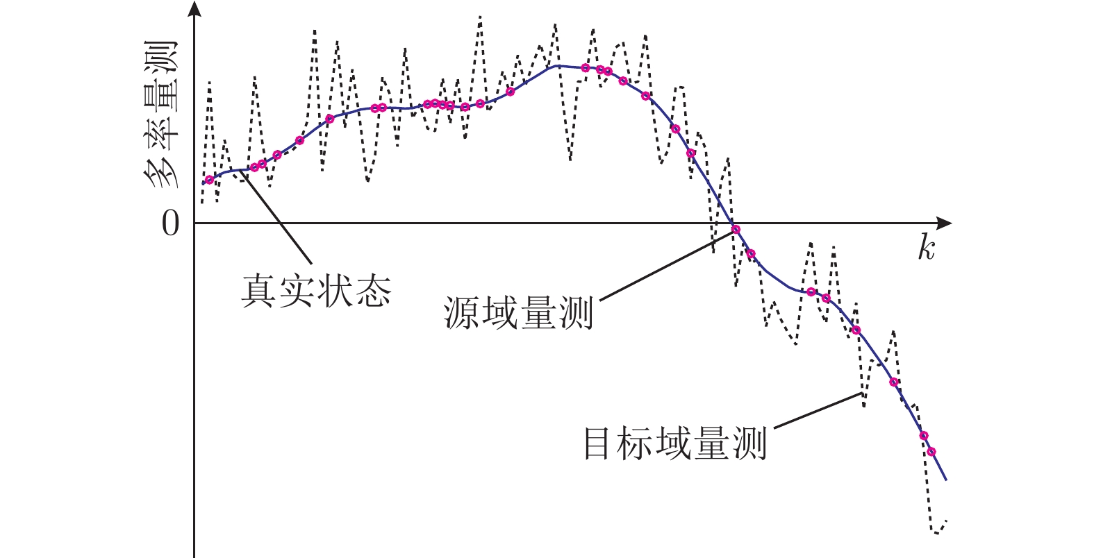
  • 图  1  多率量测过程 (实线表示真实状态, 虚线表示目标域量测 (在线快速率数据), 点表示源域量测 (离线化验数据), 其采样时间可能不规律)

    Fig.  1  Multiple source measurements of the process with different sampling rates (Solid lines are true states, and dashed lines represent target measurements. Dots denote source measurements, whose sample time may be irregular)
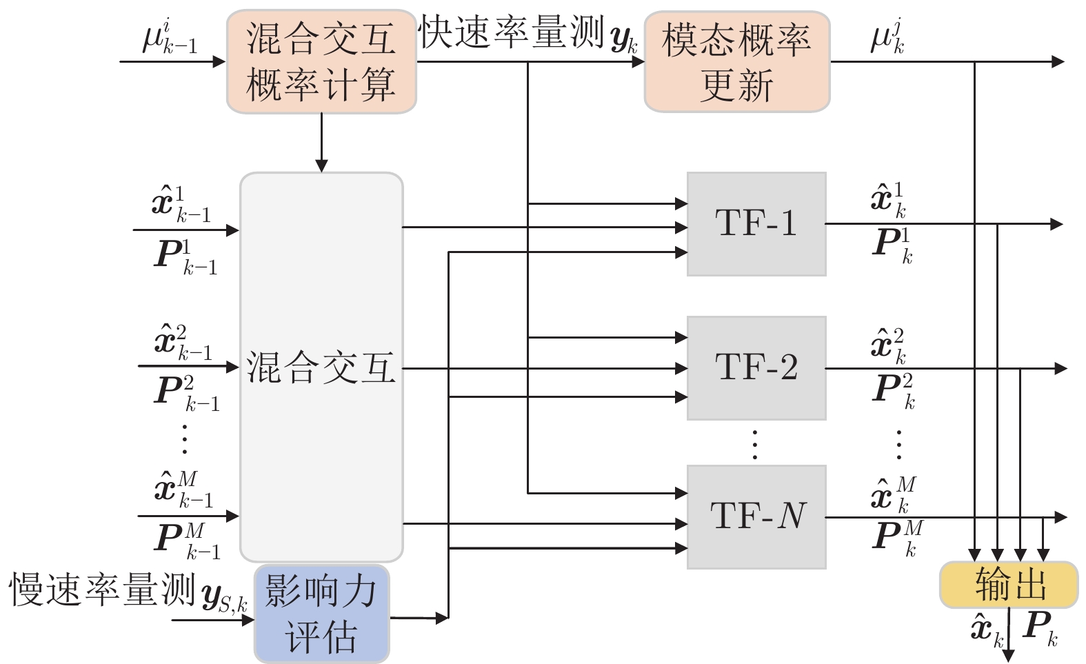
    图  2  迁移交互多模型估计器结构图

    Fig.  2  Basic operation diagram of the transfer interacting multiple model state estimator

    图  3  源域数据对迁移估计器的影响力曲线

    Fig.  3  The influence function of source measurements on the transfer state estimator

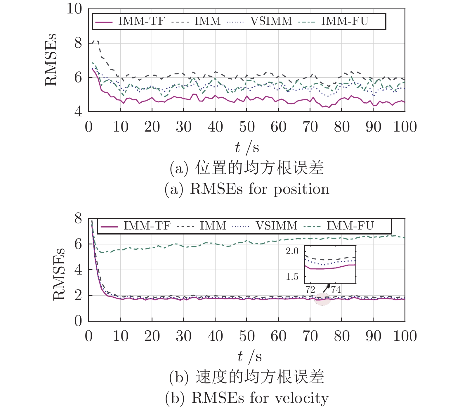
    图  4  不同算法在运动目标跟踪中的均方根误差

    Fig.  4  RMSEs of different algorithms for the moving target tracking

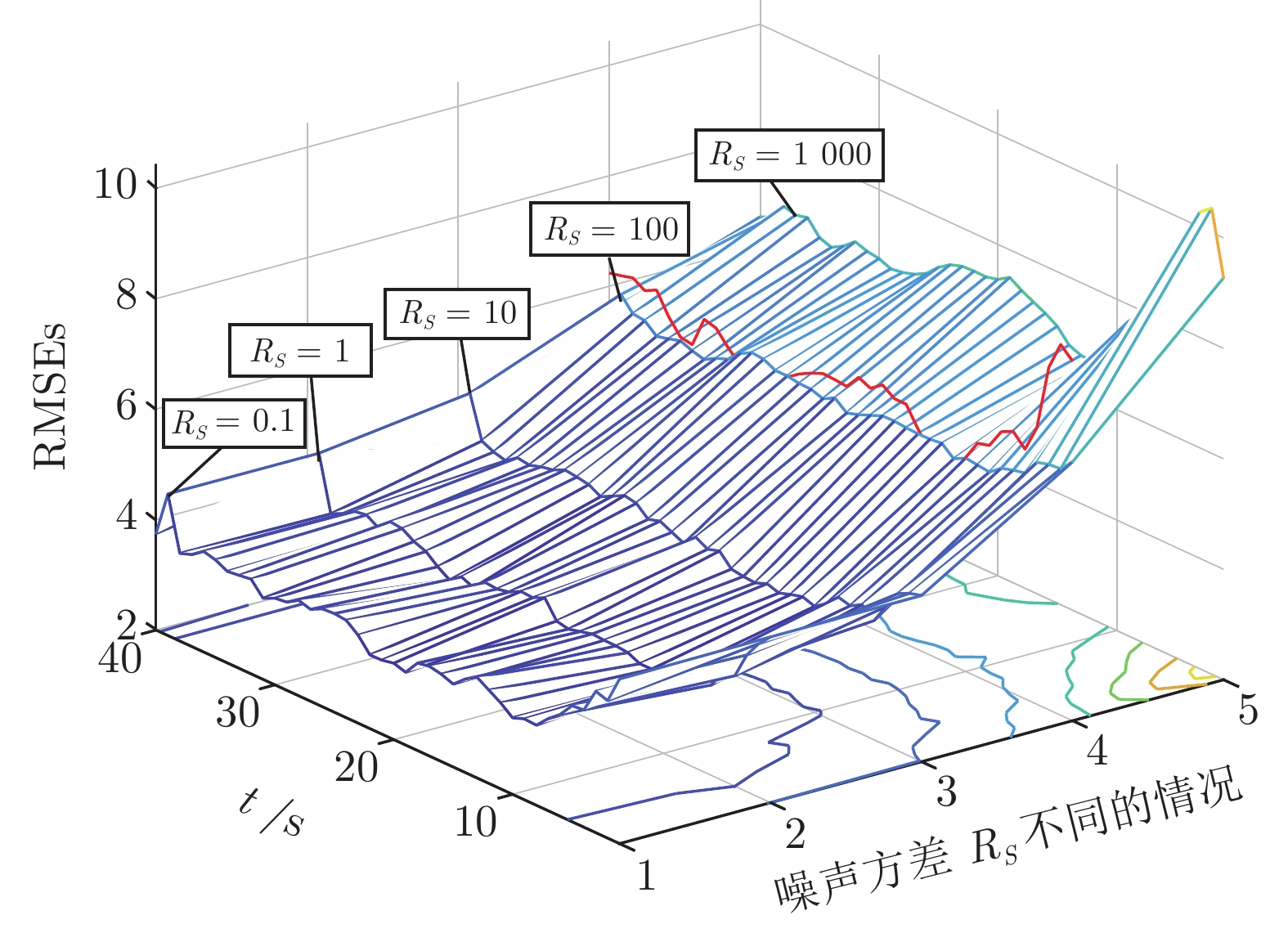
    图  5  源域数据质量对迁移估计器算法性能的影响

    Fig.  5  Demonstration of the performance of IMM-TF in the presence of source measurements of different quality

    图  6  基于影响力值的迁移估计器算法性能

    Fig.  6  Demonstration of the performance of IF-TF

    表  1  不同数量的源域数据迁移后的 RMSEs

    Table  1  Average RMSEs (per sample) of IMM-TF in the presence of different amount source measurements

    源域数据比重 (%)位置 (m)速度 (m/s)
    105.87552.0266
    305.40701.9567
    504.88681.8798
    704.53141.8465
    994.09991.7674
    下载: 导出CSV
  • [1] Wu Y, Luo X L. A novel calibration approach of soft sensor based on multirate data fusion technology. Journal of Process Control, 2010, 20(10): 1252-1260 doi: 10.1016/j.jprocont.2010.09.003
    [2] Fatehi A, Huang B. Kalman filtering approach to multi-rate information fusion in the presence of irregular sampling rate and variable measurement delay. Journal of Process Control, 2017, 53: 15-25 doi: 10.1016/j.jprocont.2017.02.010
    [3] Fatehi A, Huang B. State estimation and fusion in the presence of integrated measurement. IEEE Transactions on Instrumentation and Measurement, 2017, 66(9): 2490-2499 doi: 10.1109/TIM.2017.2701143
    [4] Gou B, Cheng Y M, de Ruiter A H J. INS/CNS navigation system based on multi-star pseudo measurements. Aerospace Science and Technology, 2019, 95: Article No. 105506 doi: 10.1016/j.ast.2019.105506
    [5] Bar-Shalom Y, Campo L. The effect of the common process noise on the two-sensor fused-track covariance. IEEE Transactions on Aerospace and Electronic Systems, 1986, 22(6): 803-805
    [6] Gao J B, Harris C J. Some remarks on Kalman filters for the multisensor fusion. Information Fusion, 2002, 3(3): 191-201 doi: 10.1016/S1566-2535(02)00070-2
    [7] Xie L, Zhu Y J, Huang B, Zheng Y S. Kalman filtering approach to multirate information fusion for soft sensor development. In: Proceedings of the 15th International Conference on Information Fusion. Singapore: IEEE, 2012. 641−648
    [8] Tian T, Sun S L. Distributed fusion estimation for multisensor multirate systems with packet dropout compensations and correlated noises. IEEE Transactions on Systems, Man, and Cybernetics: Systems, 2021, 51(9): 5762-5772 doi: 10.1109/TSMC.2019.2956259
    [9] Gopalakrishnan A, Kaisare N S, Narasimhan S. Incorporating delayed and infrequent measurements in Extended Kalman Filter based nonlinear state estimation. Journal of Process Control, 2011, 21(1): 119-129 doi: 10.1016/j.jprocont.2010.10.013
    [10] Guo Y F, Zhao Y, Huang B. Development of soft sensor by incorporating the delayed infrequent and irregular measurements. Journal of Process Control, 2014, 24(11): 1733-1739 doi: 10.1016/j.jprocont.2014.09.006
    [11] Zhou J, Zhu Y M, You Z S, Song E B. An efficient algorithm for optimal linear estimation fusion in distributed multisensor systems. IEEE Transactions on Systems, Man, and Cybernetics-Part A: Systems and Humans, 2006, 36(5): 1000-1009 doi: 10.1109/TSMCA.2006.878986
    [12] Wang D, Ha M M, Zhao M M. The intelligent critic framework for advanced optimal control. Artificial Intelligence Review, 2022, 55(1): 1-22 doi: 10.1007/s10462-021-10118-9
    [13] 王鼎, 赵明明, 哈明鸣. 基于折扣广义值迭代的智能最优跟踪及应用验证. 自动化学报, 2022, 48(1): 182-193

    Wang Ding, Zhao Ming-Ming, Ha Ming-Ming. Intelligent optimal tracking with application verifications via discounted generalized value iteration. Acta Automatica Sinica, 2022, 48(1): 182-193
    [14] Salehi Y, Fatehi A, Nayebi M A. State estimation of slow-rate integrated measurement systems in the presence of parametric uncertainties. IEEE Transactions on Instrumentation and Measurement, 2018, 68(10): 3983-3991
    [15] Lin H L, Sun S L. Distributed fusion estimator for multisensor multirate systems with correlated noises. IEEE Transactions on Systems, Man, and Cybernetics: Systems, 2017, 48(7): 1131-1139
    [16] Yan L P, Di C Y, Wu Q M J, Xia Y Q. Sequential fusion for multirate multisensor systems with heavy-tailed noises and unreliable measurements. IEEE Transactions on Systems, Man, and Cybernetics: Systems, 2020, 52(1): 523-532
    [17] Smith D, Singh S. Approaches to multisensor data fusion in target tracking: A survey. IEEE Transactions on Knowledge and Data Engineering, 2006, 18(12): 1696-1710 doi: 10.1109/TKDE.2006.183
    [18] Li W L, Jia Y M. Consensus-based distributed multiple model UKF for jump Markov nonlinear systems. IEEE Transactions on Automatic Control, 2011, 57(1): 227-233
    [19] Li W L, Jia Y M. Distributed consensus filtering for discrete-time nonlinear systems with non-Gaussian noise. Signal Processing, 2012, 92(10): 2464-2470 doi: 10.1016/j.sigpro.2012.03.009
    [20] Song H, Shin V, Jeon M. Mobile node localization using fusion prediction-based interacting multiple model in cricket sensor network. IEEE Transactions on Industrial Electronics, 2012, 59(11): 4349-4359 doi: 10.1109/TIE.2011.2151821
    [21] Fu Z, Angelini F, Chambers J, Naqvi S M. Multi-level cooperative fusion of GM-PHD filters for online multiple human tracking. IEEE Transactions on Multimedia, 2019, 21(9): 2277-2291 doi: 10.1109/TMM.2019.2902480
    [22] Shen X J, Zhu Y M, Song E B, Luo Y T. Optimal centralized update with multiple local out-of-sequence measurements. IEEE Transactions on Signal Processing, 2009, 57(4): 1551-1562 doi: 10.1109/TSP.2009.2012885
    [23] Chi X B, Jia X C, Cheng F Q, Fan M H. Networked H filtering for Takagi-Sugeno fuzzy systems under multi-output multi-rate sampling. Journal of the Franklin Institute, 2019, 356(6): 3661-3691 doi: 10.1016/j.jfranklin.2018.10.040
    [24] Zhou W D, Liu M M. Robust interacting multiple model algorithms based on multi-sensor fusion criteria. International Journal of Systems Science, 2016, 47(1): 92-106 doi: 10.1080/00207721.2015.1029566
    [25] Fu X, Jia Y, Du J, Yu F. New interacting multiple model algorithms for the tracking of the manoeuvring target. IET Control Theory and Applications, 2010, 4(10): 2184-2194 doi: 10.1049/iet-cta.2009.0583
    [26] Li Z, Teng J, Qiu J B, Gao H J. Filtering design for multirate sampled-data systems. IEEE Transactions on Systems, Man, and Cybernetics: Systems, 2020, 50(11): 4224-4232 doi: 10.1109/TSMC.2018.2839674
    [27] Li X R, Bar-Shalom Y. Multiple-model estimation with variable structure. IEEE Transactions on Automatic Control, 1996, 41(4): 478-493 doi: 10.1109/9.489270
    [28] Katsikas S K, Likothanassis S D, Beligiannis G N, Berkeris K G, Fotakis D A. Genetically determined variable structure multiple model estimation. IEEE Transactions on Signal Processing, 2001, 49(10): 2253-2261 doi: 10.1109/78.950781
    [29] Zhao S Y, Ahn C K, Shi P, Shmaliy Y S, Liu F. Bayesian state estimation for Markovian jump systems: Employing recursive steps and pseudocodes. IEEE Systems Man and Cybernetics Magazine, 2019, 5(2): 27-36 doi: 10.1109/MSMC.2018.2882145
    [30] Wen L, Gao L, Li X Y. A new deep transfer learning based on sparse auto-encoder for fault diagnosis. IEEE Transactions on Systems, Man, and Cybernetics: Systems, 2019, 49(1): 136-144 doi: 10.1109/TSMC.2017.2754287
    [31] Wang B, Li Z C, Dai Z W, Lawrence N, Yan X F. Data-driven mode identification and unsupervised fault detection for nonlinear multimode processes. IEEE Transactions on Industrial Informatics, 2019, 16(6): 3651-3661
    [32] Sun L, Ho W K, Ling K V, Chen T P, Maciejowski J. Recursive maximum likelihood estimation with t-distribution noise model. Automatica, 2021, 132: Article No. 109789 doi: 10.1016/j.automatica.2021.109789
    [33] Xue W, Luan X L, Zhao S Y, Liu F. A fusion Kalman filter and UFIR estimator using the influence function method. IEEE/CAA Journal of Automatica Sinica, 2021, 9(4): 709-718
    [34] Li X R. Multiple-model estimation with variable structure. II. Model-set adaptation. IEEE Transactions on Automatic Control, 2000, 45(11): 2047-2060 doi: 10.1109/9.887626
  • 加载中
图(6) / 表(1)
计量
  • 文章访问数:  717
  • HTML全文浏览量:  86
  • PDF下载量:  191
  • 被引次数: 0
出版历程
  • 收稿日期:  2022-01-04
  • 录用日期:  2022-07-21
  • 网络出版日期:  2022-11-02
  • 刊出日期:  2023-01-07

目录

/

返回文章
返回