

Adaptive Dynamic Programming Based Visual Servoing Tracking Control for Mobile Robots
-
摘要: 针对移动机器人视觉伺服跟踪控制问题, 提出一种基于自适应动态规划(Adaptive dynamic programming, ADP) 的控制方法. 通过移动机器人上的相机拍摄共面特征点的当前图像、期望图像以及参考图像, 利用单应性技术得到移动机器人当前的位姿信息与期望的位姿信息(即平移量与旋转角度), 从而通过当前与期望的平移旋转之间差值得到系统的开环误差模型. 进而, 针对此系统设计最优控制器, 同时做合适的控制输入变换. 在此基础上设计一个基于ADP的视觉伺服控制方法以保证移动机器人完成轨迹跟踪任务. 为求出最优控制输入, 采用一个评价神经网络近似值函数, 通过不断学习逼近哈密顿−雅可比−贝尔曼(Hamilton-Jacobi-Bellman, HJB)方程的解. 与以往不同的是, 由于系统存在时变项, 导致HJB方程也含有时变项, 因此需要设计具有时变权值结构的神经网络近似值函数. 最终证明在所设计的控制方法作用下, 闭环系统是一致最终有界的.Abstract: In this paper, a visual servoing approach based on adaptive dynamic programming (ADP) is developed for the trajectory tracking control of mobile robots. First, according to the current image, the desired image and reference image sequence of coplanar feature points are captured by the on-board camera. The current pose information and desired pose information of the mobile robot can be reconstructed by homography technology. Then, the open-loop error model of the system is obtained by the difference between the current translation and rotation and the desired. In order to design the optimal controller for this system, the appropriate control input transformation is adopted. Therefore, a visual servoing approach based on ADP is proposed to achieve the trajectory tracking task for the mobile robot. A critic neural network structure is used to learn the time-varying solution, namely the optimal value function, of the Hamilton-Jacobi-Bellman (HJB) equation. Owing to the existence of time-varying terms, which is different from many existing works, the HJB equation is time-varying. Therefore, a neural network with a time-varying weight structure is designed to approximate the time-dependent value function of the HJB equation. Finally, it is proved that the approach proposed in this paper guarantees the closed-loop system is uniformly ultimately bounded.
-
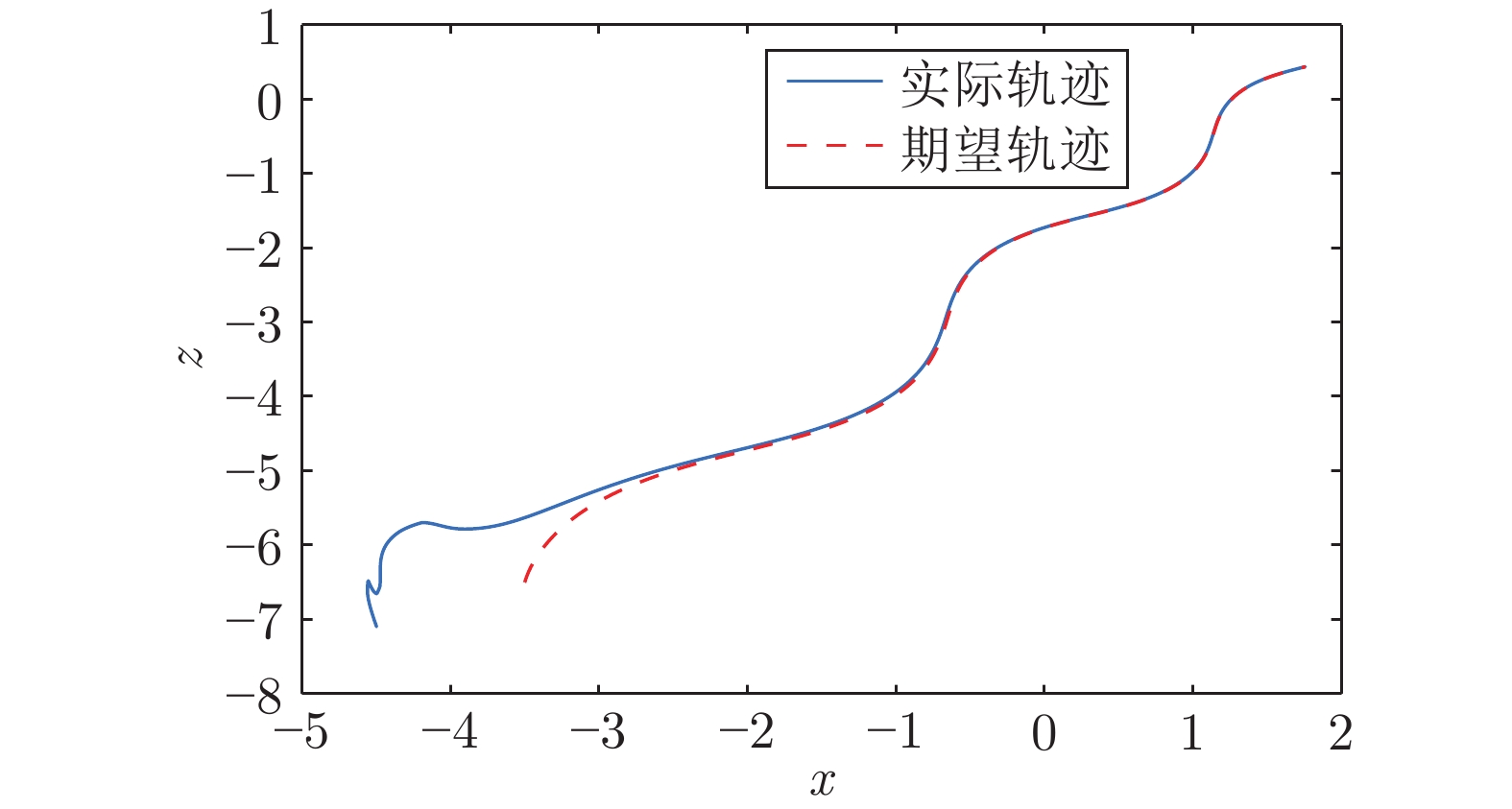
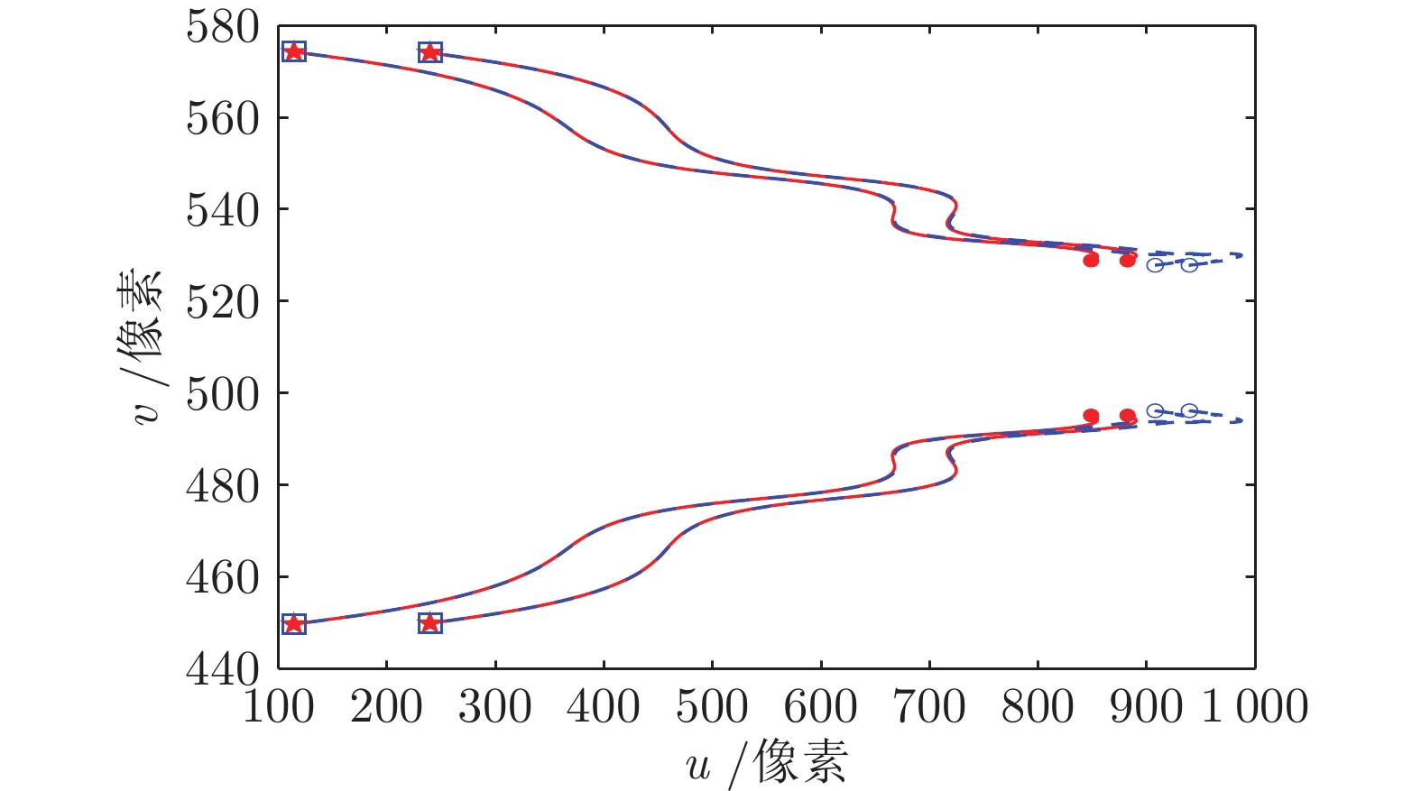
图 7 利用本文时变权值神经网络结构方法的移动机器人期望轨迹与实际运动轨迹
Fig. 7 Desired and real trajectories of the mobile robot using time-varying weights neural network structure method in this paper
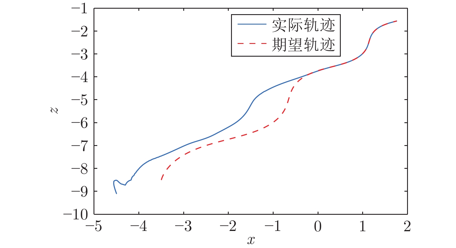
图 8 利用时变激活函数神经网络结构方法的移动机器人期望轨迹与实际运动轨迹
Fig. 8 Desired and real trajectories of the mobile robot using time-varying activation neural network structure method
-
[1] 贾丙西, 刘山, 张凯祥, 陈剑. 机器人视觉伺服研究进展: 视觉系统与控制策略. 自动化学报, 2015, 41(5): 861-873Jia Bing-Xi, Liu Shan, Zhang Kai-Xiang, Chen Jian. Survey on robot visual servo control: Vision system and control strategies. Acta Automatica Sinica, 2015, 41(5): 861-873 [2] Fomena R T, Tahri O, Chaumette F. Distance-based and orientation-based visual servoing from three points. IEEE Transactions on Robotics, 2011, 27(2): 256-267 doi: 10.1109/TRO.2011.2104431 [3] 杨芳, 王朝立. 基于视觉伺服反馈的不确定非完整动态移动机器人的自适应镇定. 自动化学报, 2011, 37(7): 857-864 doi: 10.1016/S1874-1029(11)60211-5Yang Fang, Wang Chao-Li. Adaptive stabilization for uncertain nonholonomic dynamic mobile robots based on visual servoing feedback. Acta Automatica Sinica, 2011, 37(7): 857-864 doi: 10.1016/S1874-1029(11)60211-5 [4] Jiang Z P. Robust exponential regulation of nonholonomic systems with uncertainties. Automatica, 2000, 36(2): 189-209 doi: 10.1016/S0005-1098(99)00115-6 [5] Chen, J, Dixon, W E, Dawson, D M, McIntire, M. Homography-based visual servo tracking control of a wheeled mobile robot. IEEE Transactions on Robotics, 2006, 22(2): 406-415 doi: 10.1109/TRO.2006.862476 [6] Liang X, Wang H, Chen W, Guo D, Liu T. Adaptive image-based trajectory tracking control of wheeled mobile robots with an uncalibrated fixed camera. IEEE Transactions on Control Systems Technology, 2015, 23(6): 2266-2282 doi: 10.1109/TCST.2015.2411627 [7] 徐德. 单目视觉伺服研究综述. 自动化学报, 2018, 44(10): 1729-1746Xu De. A tutorial for monocular visual servoing. Acta Automatica Sinica, 2018, 44(10): 1729-1746 [8] Brockett R W, Millman R S, Sussmann H J. Differential Geometric Control Theory. Michigan: Birkhauser Boston, 1983. [9] Jiang Z P, Nijmeijer H. Tracking control of mobile robots: A case study in backstepping. Automatica, 1997, 33(7): 1393-1399 doi: 10.1016/S0005-1098(97)00055-1 [10] Li B, Fang Y, Hu G, Zhang X. Model-free unified tracking and regulation visual servoing of wheeled mobile robots. IEEE Transactions on Control Systems Technology, 2015, 24(4): 1328-1339 [11] Li L, Liu Y H, Jiang T, Wang K, Fang M. Adaptive trajectory tracking of nonholonomic mobile robots using vision-based position and velocity estimation. IEEE Transactions on Cybernetics, 2017, 48(2): 571-582 [12] Miao Z, Zhong H, Lin J, Wang Y, Chen Y, Fierro R. Vision-based bormation control of mobile robots with FOV constraints and unknown feature depth. IEEE Transactions on Control Systems Technology, 2021, 29(5): 2231-2238 doi: 10.1109/TCST.2020.3023415 [13] Zhang K, Chen J, Li Y, Zhang X. Visual tracking and depth estimation of mobile robots without desired velocity information. IEEE Transactions on Cybernetics, 2020, 50(1): 361-373 doi: 10.1109/TCYB.2018.2869623 [14] Lee S, Chwa D. Dynamic image-based visual servoing of monocular camera mounted omnidirectional mobile robots considering actuators and target motion via fuzzy integral sliding mode control. IEEE Transactions on Fuzzy Systems, 2021, 29(7): 2068-2076 doi: 10.1109/TFUZZ.2020.2985931 [15] Wang R, Zhang X, Fang Y, Li B. Virtual-goal-guided RRT for visual servoing of mobile robots with FOV constraint. IEEE Transactions on Systems, Man, and Cybernetics: Systems, 2022, 52(4): 2073-2083 doi: 10.1109/TSMC.2020.3044347 [16] Kiumarsi B, Lewis F L. Actor-critic-based optimal tracking for partially unknown nonlinear discrete-time systems. IEEE Transactions on Neural Networks and Learning Systems, 2014, 26(1): 140-151 [17] Luo B, Wu H N, Li H X. Adaptive optimal control of highly dissipative nonlinear spatially distributed processes with neuro-dynamic programming. IEEE Transactions on Neural Networks and Learning Systems, 2015, 26(4): 684-696 doi: 10.1109/TNNLS.2014.2320744 [18] Liu D, Xue S, Zhao B, Luo B, Wei Q. Adaptive dynamic programming for control: A survey and recent advances. IEEE Transactions on Systems, Man, and Cybernetics: Systems, 2021, 51(1): 142-160 doi: 10.1109/TSMC.2020.3042876 [19] Ming Z, Zhang H, Yan Y, Zhang J. Tracking control of discrete-time system with dynamic event-based adaptive dynamic programming. IEEE Transactions on Circuits and Systems II: Express Briefs, 2022, 69(8): 3570-3574 doi: 10.1109/TCSII.2022.3168428 [20] Li S, Ding L, Gao H, Liu Y J, Huang L, Deng Z. ADP-based online tracking control of partially uncertain time-delayed nonlinear system and application to wheeled mobile robots. IEEE Transactions on Cybernetics, 2020, 50(7): 3182-3194 doi: 10.1109/TCYB.2019.2900326 [21] Kong L, He W, Yang C, Sun C. Robust neurooptimal control for a robot via adaptive dynamic programming. IEEE Transactions on Neural Networks and Learning Systems, 2021, 32(6): 2584-2594 doi: 10.1109/TNNLS.2020.3006850 [22] 张化光, 张欣, 罗艳红, 杨珺. 自适应动态规划综述. 自动化学报, 2013, 39(4): 303-311 doi: 10.1016/S1874-1029(13)60031-2Zhang Hua-Guang, Zhang Xin, Luo Yan-Hong, Yang Jun. An overview of research on adaptive dynamic programming. Acta Automatica Sinica, 2013, 39(4): 303-311 doi: 10.1016/S1874-1029(13)60031-2 [23] Liu D, Wang D, Wang F Y, Li H, Yang, X. Neural-network-based online HJB solution for optimal robust guaranteed cost control of continuous-time uncertain nonlinear systems. IEEE Transactions on Cybernetics, 2014, 44(12): 2834-2847 doi: 10.1109/TCYB.2014.2357896 [24] 王鼎, 穆朝絮, 刘德荣. 基于迭代神经动态规划的数据驱动非线性近似最优调节. 自动化学报, 2017, 43(3): 366-375 doi: 10.16383/j.aas.2017.c160272Wang Ding, Mu Chao-Xu, Liu De-Rong. Data-driven nonlinear near-optimal regulation based on iterative neural dynamic programming. Acta Automatica Sinica, 2017, 43(3): 366-375 doi: 10.16383/j.aas.2017.c160272 [25] Bhasin S, Kamalapurkar R, Johnson M, Vamvoudakis K G, Lewis F L, Dixon W E. A novel actor-critic-identifier architecture for approximate optimal control of uncertain nonlinear systems. Automatica, 2013, 49(1): 82-92 doi: 10.1016/j.automatica.2012.09.019 [26] Lin W S, Yang P C. Adaptive critic motion control design of autonomous wheeled mobile robot by dual heuristic programming. Automatica, 2008, 44(11): 2716-2723 doi: 10.1016/j.automatica.2008.03.029 [27] Cheng T, Lewis F L, Abu-Khalaf M. A neural network solution for fixed-final time optimal control of nonlinear systems. Automatica, 2007, 43(3): 482-490 doi: 10.1016/j.automatica.2006.09.021 [28] Heydari A, Balakrishnan S N. Fixed-final-time optimal tracking control of input-affine nonlinear systems. Neurocomputing, 2014, 129(10): 528-539 [29] Wang F Y, Jin N, Liu D, Wei Q. Adaptive dynamic programming for finite-horizon optimal control of discrete-time nonlinear systems with ε-error bound. IEEE Transactions on Neural Networks, 2010, 22(1): 24-36 [30] Zhao Q, Xu H, Jagannathan S. Neural network-based finite-horizon optimal control of uncertain affine nonlinear discrete-time systems. IEEE Transactions on Neural Networks and Learning Systems, 2014, 26(3): 486-499 [31] Hartley R, Zisserman A. Multiple View Geometry in Computer Vision. Cambridge: Cambridge University Press, 2003. [32] Siciliano B, Sciavicco L, Villani L, Oriolo G. Robotics: Modelling, Planning and Control. London: Springer-Verlag, 2009. [33] Zhang K, Chen J, Li Y, Zhang X. Visual tracking and depth estimation of mobile robots without desired velocity information. IEEE Transactions on Cybernetics, 2018, 50(1): 361-373 [34] Lewis F L, Vrabie D L, Syrmos V L. Optimal Control, Third Edition. Hoboken: John Wiley & Sons, 2012. [35] Finlayson B A. The Method of Weighted Residuals and Variational Principles. Philadelphia: Society for Industrial and Applied Mathematics, 2013. [36] Abu-Khalaf M, Lewis F L. Nearly optimal control laws for nonlinear systems with saturating actuators using a neural network HJB approach. Automatica, 2005, 41(5): 779-791 doi: 10.1016/j.automatica.2004.11.034 [37] Pakkhesal S, Shamaghdari S. Sum-of-squares-based policy iteration for suboptimal control of polynomial time-varying systems. Asian Journal of Control, 2022, 24(6): 3022-3031 doi: 10.1002/asjc.2689 [38] Wei Q, Liao Z, Yang Z, Li B, Liu D. Continuous-time time-varying policy iteration. IEEE Transactions on Cybernetics, 2020, 50(12): 4958-4971 doi: 10.1109/TCYB.2019.2926631 [39] Zhang H, Cui L, Zhang X, Luo Y. Data-driven robust approximate optimal tracking control for unknown general nonlinear systems using adaptive dynamic programming method. IEEE Transactions on Neural Networks, 2011, 22(12): 2226-2236 doi: 10.1109/TNN.2011.2168538 -

 下载:
下载:


图(9)
计量
- 文章访问数: 1886
- HTML全文浏览量: 846
- PDF下载量: 555
- 被引次数: 0
