

-
摘要: 图像的模糊问题影响人们对信息的感知、获取及图像的后续处理. 无参考模糊图像质量评价是该问题的主要研究方向之一. 本文分析了近20年来无参考模糊图像质量评价相关技术的发展. 首先, 本文结合主要数据集对图像模糊失真进行分类说明; 其次, 对主要的无参考模糊图像质量评价方法进行分类介绍与详细分析; 随后, 介绍了用来比较无参考模糊图像质量评价方法性能优劣的主要评价指标; 接着, 选择典型数据集及评价指标, 并采用常见的无参考模糊图像质量评价方法进行性能比较; 最后, 对无参考模糊图像质量评价的相关技术及发展趋势进行总结与展望.Abstract: The blurriness distortion of image affects information perception, acquisition and subsequent processing. No-reference blurred image quality assessment is one of main research directions for the problem. This paper analyzes the relevant technique development of no-reference blurred image quality assessment in recent 20 years. Firstly, combining with main databases, different types of blurriness distortions are described. Secondly, main methods for no-reference blurred image quality assessment are classified and analyzed in detail. Thirdly, performance measures for no-reference blurred image assessment are introduced. Then, the typical databases, performance measures and methods are introduced for performance comparisons. Finally, the relevant technologies and development trends of no-reference blurred image assessment are summarized and prospected.
-
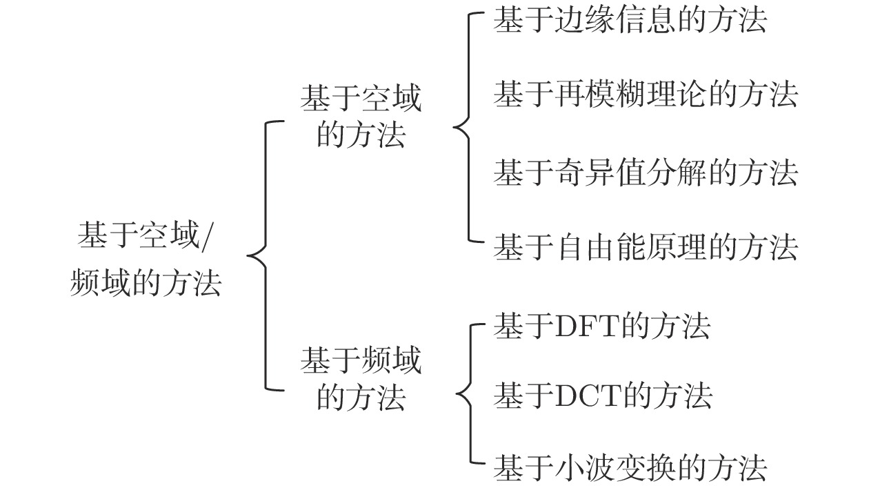
图 2 基于空域/频域的NR-IQA方法分类
Fig. 2 Classification of spatial/spectral domain-based NR-IQA methods
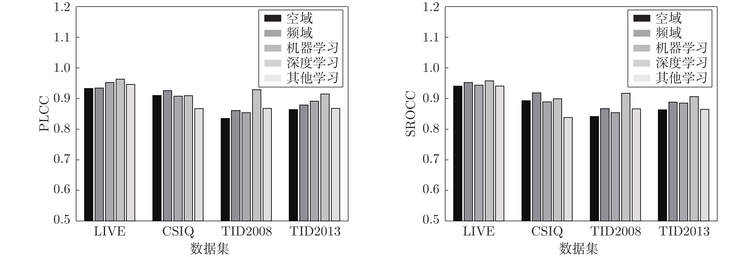
图 4 不同类型NR-IQA方法在不同人工模糊数据集中平均性能评价指标值比较
Fig. 4 Average performance evaluation result comparison through different types of NR-IQA methods for different artificial blur databases
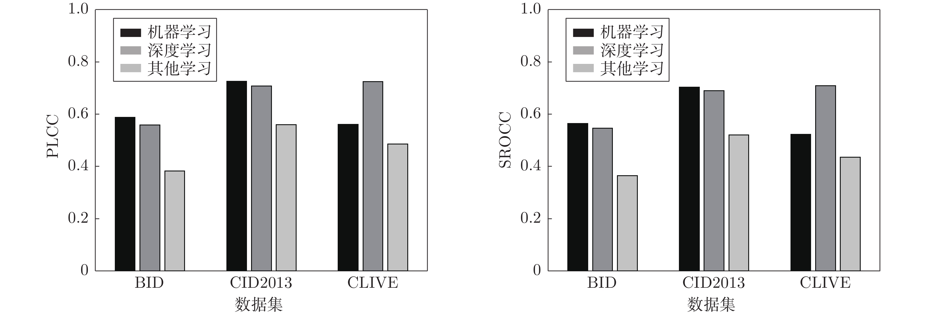
图 5 不同类型NR-IQA方法在不同自然模糊数据集中平均性能评价指标值比较
Fig. 5 Average performance evaluation result comparison through different types of NR-IQA methods for different natural blur databases
表 1 含有模糊图像的主要图像质量评价数据集
Table 1 Main image quality assessment databases including blurred images
数据集 时间 参考图像 模糊图像 模糊类型 主观评价 分值范围 IVC[28] 2005 4 20 高斯模糊 MOS 模糊−清晰 [1 5] LIVE[22] 2006 29 145 高斯模糊 DMOS 清晰−模糊 [0 100] A57[30] 2007 3 9 高斯模糊 DMOS 清晰−模糊 [0 1] TID2008[26] 2009 25 100 高斯模糊 MOS 模糊−清晰 [0 9] CSIQ[25] 2009 30 150 高斯模糊 DMOS 清晰−模糊 [0 1] VCL@FER[29] 2012 23 138 高斯模糊 MOS 模糊−清晰 [0 100] TID2013[27] 2013 25 125 高斯模糊 MOS 模糊−清晰 [0 9] KADID-10k 1[31] 2019 81 405 高斯模糊 MOS 模糊−清晰 [1 5] KADID-10k 2[31] 2019 81 405 镜头模糊 MOS 模糊−清晰 [1 5] KADID-10k 3[31] 2019 81 405 运动模糊 MOS 模糊−清晰 [1 5] MLIVE1[33] 2012 15 225 高斯模糊和高斯白噪声 DMOS 清晰−模糊 [0 100] MLIVE2[33] 2012 15 225 高斯模糊和JEPG压缩 DMOS 清晰−模糊 [0 100] MDID2013[32] 2013 12 324 高斯模糊、JEPG压缩和白噪声 DMOS 清晰−模糊 [0 1] MDID[34] 2017 20 1600 高斯模糊、对比度变化、高斯噪声、
JPEG或JPEG2000MOS 模糊−清晰 [0 8] BID[21] 2011 — 586 自然模糊 MOS 模糊−清晰 [0 5] CID2013[35] 2013 — 480 自然模糊 MOS 模糊−清晰 [0 100] CLIVE[36-37] 2016 — 1162 自然模糊 MOS 模糊−清晰 [0 100] KonIQ-10k [38] 2018 — 10073 自然模糊 MOS 模糊−清晰 [1 5]  下载: 导出CSV
表 2 基于空域/频域的不同方法优缺点对比
Table 2 Advantage and disadvantage comparison for different methods based on spatial/spectral domain
方法分类 优点 缺点 边缘信息 概念直观、计算复杂度低 容易因图像中缺少锐利边缘而影响评价结果 再模糊理论 对图像内容依赖小, 计算复杂度低 准确性依赖 FR-IQA 方法 奇异值分解 能较好地提取图像结构、边缘、纹理信息 计算复杂度较高 自由能理论 外部输入信号与其生成模型可解释部分之间的
差距与视觉感受的图像质量密切相关计算复杂度高 DFT/DCT/小波变换 综合了图像的频域特性和多尺度特征, 准确性和鲁棒性更高 计算复杂度高
下载: 导出CSV
表 3 基于学习的不同方法优缺点对比
Table 3 Advantage and disadvantage comparison for different methods based on learning
方法分类 优点 缺点 SVM 在小样本训练集上能够取得比其他算法更好的效果 评价结果的好坏由提取的特征决定 NN 具有很好的非线性映射能力 样本较少时, 容易出现过拟合现象, 且
计算复杂度随着数据量的增加而增大深度学习 可以从大量数据中自动学习图像特征的多层表示 对数据集中数据量要求大 字典/码本 可以获得图像中的高级特征 字典/码本的大小减小时, 性能显著下降 MVG 无需图像的 MOS/DMOS 值 模型建立困难, 对数据集中数据量要求较大
下载: 导出CSV
表 4 用于对比的不同NR-IQA方法
Table 4 Different NR-IQA methods for comparison
方法类别 方法 特征 模糊/通用 空域/频域 空域 边缘信息 JNB[43] 计算边缘分块所对应的边缘宽度 模糊 边缘信息 CPBD[44] 计算模糊检测的累积概率 模糊 边缘信息 MLV[47] 计算图像的最大局部变化得到反映图像对比度信息的映射图 模糊 自由能理论 ARISM[63] 每个像素 AR 模型系数的能量差和对比度差 模糊 边缘信息 BIBLE[49] 图像的梯度和 Tchebichef 矩量 模糊 边缘信息 Zhan 等[14] 图像中最大梯度及梯度变化量 模糊 频域 DFT变换 S3[65] 在频域测量幅度谱的斜率, 在空域测量空间变化情况 模糊 小波变换 LPC-SI[81] LPC 强度变化作为指标 模糊 小波变换 BISHARP[77] 计算图像的均方根来获取图像局部对比度信息,
同时利用小波变换中对角线小波系数模糊 HVS滤波器 HVS-MaxPol[85] 利用 MaxPol 卷积滤波器分解与图像清晰度相关的有意义特征 模糊 学习 机器学习 SVM+SVR BIQI[86] 对图像进行小波变换后, 利用 GGD 对得到的子带系数进行参数化 通用 SVM+SVR DIIVINE[87] 从小波子带系数中提取一系列的统计特征 通用 SVM+SVR SSEQ[88] 空间−频域熵特征 通用 SVM+SVR BLIINDS-II[91] 多尺度下的广义高斯模型形状参数特征、频率变化系数特征、
能量子带特征、基于定位模型的特征通用 SVR BRISQUE[96] GGD 拟合 MSCN 系数作为特征, AGGD 拟合 4 个相邻元素乘积系数作为特征 通用 SVR RISE[107] 多尺度图像空间中的梯度值和奇异值特征, 以及多分辨率图像的熵特征 模糊 SVR Liu 等[109] 局部模式算子提取图像结构信息, Toggle 算子提取边缘信息 模糊 SVR Cai 等[110] 输入图像与其重新模糊版本之间的 Log-Gabor 滤波器响应差异和基于方向
选择性的模式差异, 以及输入图像与其 4 个下采样图像之间的自相似性模糊 深度学习 CNN Kang's CNN[116] 对图像分块进行局部对比度归一化 通用 浅层CNN+GRNN Yu's CNN[127] 对图像分块进行局部对比度归一化 模糊 聚类技术+RBM MSFF[139] Gabor 滤波器提取不同方向和尺度的原始图像特征,
然后由 RBMs 生成特征描述符通用 DNN MEON[132] 原始图像作为输入 通用 CNN DIQaM-NR[131] 使用 CNN 提取失真图像块和参考图像块的特征 通用 CNN DIQA[118] 图像归一化后, 通过下采样及上采样得到低频图像 通用 CNN SGDNet[133] 使用 DCNN 作为特征提取器获取图像特征 通用 秩学习 Rank Learning[141] 选取一定比例的图像块集合作为输入, 梯度信息被用来指导图像块选择过程 模糊 DCNN+SFA SFA[128] 多个图像块作为输入, 并使用预先训练好的 DCNN 模型提取特征 模糊 DNN+NSS NSSADNN[134] 每个图像块归一化后用 CNNs 提取特征, 得到 1024 维向量 通用 CNN DB-CNN[123] 用预训练的 S-CNN 及 VGG-16 分别提取合成失真与真实图像的相关特征 通用 CNN CGFA-CNN[124] 用 VGG-16 以提取失真图像的相关特征 通用 字典/码本 聚类算法+码本 CORNIA[145] 未标记图像块中提取局部特征进行 K-means 聚类以构建码本 通用 聚类算法+码本 QAC[147] 用比例池化策略估计每个分块的局部质量,
通过 QAC 学习不同质量级别上的质心作为码本通用 稀疏学习+字典 SPARISH[143] 以图像块的方式表示模糊图像, 并使用稀疏系数计算块能量 模糊 MVG MVG模型 NIQE[150] 提取 MSCN 系数, 再用 GGD 和 AGGD 拟合得到特征 通用
下载: 导出CSV
表 5 基于深度学习的方法所采用的不同网络结构
Table 5 Different network structures of deep learning-based methods
方法 网络结构 Kang's CNN[116] 包括一个含有最大/最小池化的卷积层, 两个全连接层及一个输出结点 Yu's CNN[127] 采用单一特征层挖掘图像内在特征, 利用 GRNN 评价图像质量 MSFF[139] 图像的多个特征作为输入, 通过端到端训练学习特征权重 MEON[132] 由失真判别网络和质量预测网络两个子网络组成, 并采用 GDN 作为激活函数 DIQaM-NR[131] 包含 10 个卷积层和 5 个池化层用于特征提取, 以及 2 个全连接层进行回归分析 DIQA[118] 网络训练分为客观失真部分及与人类视觉系统相关部分两个阶段 SGDNet[133] 包括视觉显著性预测和图像质量预测的两个子任务 Rank Learning[141] 结合了 Siamese Mobilenet 及多尺度 patch 提取方法 SFA[128] 包括 4 个步骤: 图像的多 patch 表示, 预先训练好的 DCNN 模型提取特征,
通过 3 种不同统计结构进行特征聚合, 部分最小二乘回归进行质量预测NSSADNN[134] 采用多任务学习方式设计, 包括自然场景统计 (NSS) 特征预测任务和质量分数预测任务 DB-CNN[123] 两个卷积神经网络分别专注于两种失真图像特征提取, 并采用双线性池化实现质量预测 CGFA-CNN[124] 采用两阶段策略, 首先基于 VGG-16 网络的子网络 1 识别图像中的失真类型, 而后利用子网络 2 实现失真量化
下载: 导出CSV
表 6 基于空域/频域的不同NR-IQA方法在不同数据集中比较结果
Table 6 Comparison of different spatial/spectral domain-based NR-IQA methods for different databases
方法 发表时间 LIVE CSIQ PLCC SROCC RMSE MAE PLCC SROCC RMSE MAE JNB[43] 2009 0.843 0.842 11.706 9.241 0.786 0.762 0.180 0.122 CPBD[44] 2011 0.913 0.943 8.882 6.820 0.874 0.885 0.140 0.111 S3[65] 2012 0.919 0.963 8.578 7.335 0.894 0.906 0.135 0.110 LPC-SI[81] 2013 0.907 0.923 9.177 7.275 0.923 0.922 0.111 0.093 MLV[47] 2014 0.959 0.957 6.171 4.896 0.949 0.925 0.091 0.071 ARISM[63] 2015 0.962 0.968 5.932 4.512 0.944 0.925 0.095 0.076 BIBLE[49] 2016 0.963 0.973 5.883 4.605 0.940 0.913 0.098 0.077 Zhan 等[14] 2018 0.960 0.963 6.078 4.697 0.967 0.950 0.073 0.057 BISHARP[77] 2018 0.952 0.960 6.694 5.280 0.942 0.927 0.097 0.078 HVS-MaxPol[85] 2019 0.957 0.960 6.318 5.076 0.943 0.921 0.095 0.077 方法 发表时间 TID2008 TID2013 PLCC SROCC RMSE MAE PLCC SROCC RMSE MAE JNB[43] 2009 0.661 0.667 0.881 0.673 0.695 0.690 0.898 0.687 CPBD[44] 2011 0.820 0.841 0.672 0.524 0.854 0.852 0.649 0.526 S3[65] 2012 0.851 0.842 0.617 0.478 0.879 0.861 0.595 0.480 LPC-SI[81] 2013 0.861 0.896 0.599 0.478 0.869 0.919 0.621 0.507 MLV[47] 2014 0.858 0.855 0.602 0.468 0.883 0.879 0.587 0.460 ARISM[63] 2015 0.843 0.851 0.632 0.492 0.895 0.898 0.558 0.442 BIBLE[49] 2016 0.893 0.892 0.528 0.413 0.905 0.899 0.531 0.426 Zhan 等[14] 2018 0.937 0.942 0.410 0.320 0.954 0.961 0.374 0.288 BISHARP[77] 2018 0.877 0.880 0.564 0.439 0.892 0.896 0.565 0.449 HVS-MaxPol[85] 2019 0.853 0.851 0.612 0.484 0.877 0.875 0.599 0.484
下载: 导出CSV
表 7 基于学习的不同NR-IQA方法在不同人工模糊数据集中比较结果
Table 7 Comparison of different learning-based NR-IQA methods for different artificial blur databases
方法 发表
时间LIVE CSIQ TID2008 TID2013 PLCC SROCC PLCC SROCC PLCC SROCC PLCC SROCC BIQI[86] 2010 0.920 0.914 0.846 0.773 0.794 0.799 0.825 0.815 DIIVINE[87] 2011 0.943 0.936 0.886 0.879 0.835 0.829 0.847 0.842 BLIINDS-II[91] 2012 0.939 0.931 0.886 0.892 0.842 0.859 0.857 0.862 BRISQUE[96] 2012 0.951 0.943 0.921 0.907 0.866 0.865 0.862 0.861 CORNIA[145] 2012 0.968 0.969 0.781 0.714 0.932 0.932 0.904 0.912 NIQE[150] 2013 0.939 0.930 0.918 0.891 0.832 0.823 0.816 0.807 QAC[147] 2013 0.916 0.903 0.831 0.831 0.813 0.812 0.848 0.847 SSEQ[88] 2014 0.961 0.948 0.871 0.870 0.858 0.852 0.863 0.862 Kang's CNN[116] 2014 0.963 0.983 0.774 0.781 0.880 0.850 0.931 0.922 SPARISH[143] 2016 0.960 0.960 0.939 0.914 0.896 0.896 0.902 0.894 Yu's CNN[127] 2017 0.973 0.965 0.942 0.925 0.937 0.919 0.922 0.914 RISE[107] 2017 0.962 0.949 0.946 0.928 0.929 0.922 0.942 0.934 MEON[132] 2018 0.948 0.940 0.916 0.905 — — 0.891 0.880 DIQaM-NR[131] 2018 0.972 0.960 0.893 0.885 — — 0.915 0.908 DIQA[118] 2019 0.952 0.951 0.871 0.865 — — 0.921 0.918 SGDNet[133] 2019 0.946 0.939 0.866 0.860 — — 0.928 0.914 Rank Learning[141] 2019 0.969 0.954 0.979 0.953 0.959 0.949 0.965 0.955 SFA[128] 2019 0.972 0.963 — — 0.946 0.937 0.954 0.948 NSSADNN[134] 2019 0.971 0.981 0.923 0.930 — — 0.857 0.840 CGFA-CNN[124] 2020 0.974 0.968 0.955 0.941 — — — — MSFF[139] 2020 0.954 0.962 — — 0.925 0.928 0.921 0.928 DB-CNN[123] 2020 0.956 0.935 0.969 0.947 — — 0.857 0.844 Liu 等[109] 2020 0.980 0.973 0.955 0.936 — — 0.972 0.964 Cai 等[110] 2020 0.958 0.955 0.952 0.923 — — 0.957 0.941
下载: 导出CSV
表 8 基于学习的不同NR-IQA方法在不同自然模糊数据集中比较结果
Table 8 Comparison of different learning-based NR-IQA methods for different natural blur databases
方法 发表
时间BID CID2013 CLIVE PLCC SROCC PLCC SROCC PLCC SROCC BIQI[86] 2010 0.604 0.572 0.777 0.744 0.540 0.519 DIIVINE[87] 2011 0.506 0.489 0.499 0.477 0.558 0.509 BLIINDS-II[91] 2012 0.558 0.530 0.731 0.701 0.507 0.463 BRISQUE[96] 2012 0.612 0.590 0.714 0.682 0.645 0.607 CORNIA[145] 2012 — — 0.680 0.624 0.665 0.618 NIQE[150] 2013 0.471 0.469 0.693 0.633 0.478 0.421 QAC[147] 2013 0.321 0.318 0.187 0.162 0.318 0.298 SSEQ[88] 2014 0.604 0.581 0.689 0.676 — — Kang's CNN[116] 2014 0.498 0.482 0.523 0.526 0.522 0.496 SPARISH[143] 2016 0.356 0.307 0.678 0.661 0.484 0.402 Yu's CNN[127] 2017 0.560 0.557 0.715 0.704 0.501 0.502 RISE[107] 2017 0.602 0.584 0.793 0.769 0.555 0.515 MEON[132] 2018 0.482 0.470 0.703 0.701 0.693 0.688 DIQaM-NR[131] 2018 0.476 0.461 0.686 0.674 0.601 0.606 DIQA[118] 2019 0.506 0.492 0.720 0.708 0.704 0.703 SGDNet[133] 2019 0.422 0.417 0.653 0.644 0.872 0.851 Rank Learning[141] 2019 0.751 0.719 0.863 0.836 — — SFA[128] 2019 0.840 0.826 — — 0.833 0.812 NSSADNN[134] 2019 0.574 0.568 0.825 0.748 0.813 0.745 CGFA-CNN[124] 2020 — — — — 0.846 0.837 DB-CNN[123] 2020 0.475 0.464 0.686 0.672 0.869 0.851 Cai 等[110] 2020 0.633 0.603 0.880 0.874 — —
下载: 导出CSV
-
[1] Jayageetha J, Vasanthanayaki C. Medical image quality assessment using CSO based deep neural network. Journal of Medical Systems, 2018, 42(11): Article No. 224 [2] Ma J J, Nakarmi U, Kin C Y S, Sandino C M, Cheng J Y, Syed A B, et al. Diagnostic image quality assessment and classification in medical imaging: Opportunities and challenges. In: Proceedings of the 17th International Symposium on Biomedical Imaging (ISBI). Iowa City, USA: IEEE, 2020. 337−340 [3] Chen G B, Zhai M T. Quality assessment on remote sensing image based on neural networks. Journal of Visual Communication and Image Representation, 2019, 63: Article No. 102580 [4] Hombalimath A, Manjula H T, Khanam A, Girish K. Image quality assessment for iris recognition. International Journal of Scientific and Research Publications, 2018, 8(6): 100-103 [5] Zhai G T, Min X K. Perceptual image quality assessment: A survey. Science China Information Sciences, 2020, 63(11): Article No. 211301 [6] 王烨茹. 基于数字图像处理的自动对焦方法研究 [博士学位论文], 浙江大学, 中国, 2018.Wang Ye-Ru. Research on Auto-focus Methods Based on Digital Imaging Processing [Ph.D. dissertation], Zhejiang University, China, 2018. [7] 尤玉虎, 刘通, 刘佳文. 基于图像处理的自动对焦技术综述. 激光与红外, 2013, 43(2): 132-136 doi: 10.3969/j.issn.1001-5078.2013.02.003You Yu-Hu, Liu Tong, Liu Jia-Wen. Survey of the auto-focus methods based on image processing. Laser and Infrared, 2013, 43(2): 132-136 doi: 10.3969/j.issn.1001-5078.2013.02.003 [8] Cannon M. Blind deconvolution of spatially invariant image blurs with phase. IEEE Transactions on Acoustics, Speech, and Signal Processing, 1976, 24(1): 58-63 doi: 10.1109/TASSP.1976.1162770 [9] Tekalp A M, Kaufman H, Woods J W. Identification of image and blur parameters for the restoration of noncausal blurs. IEEE Transactions on Acoustics, Speech, and Signal Processing, 1986, 34(4): 963-972 doi: 10.1109/TASSP.1986.1164886 [10] Pavlovic G, Tekalp A M. Maximum likelihood parametric blur identification based on a continuous spatial domain model. IEEE Transactions on Image Processing, 1992, 1(4): 496-504 doi: 10.1109/83.199919 [11] Kim S K, Park S R, Paik J K. Simultaneous out-of-focus blur estimation and restoration for digital auto-focusing system. IEEE Transactions on Consumer Electronics, 1998, 44(3): 1071-1075 doi: 10.1109/30.713236 [12] Sada M M, Mahesh G M. Image deblurring techniques-a detail review. International Journal of Scientific Research in Science, Engineering and Technology, 2018, 4(2): 176-188 [13] Wang R X, Tao D C. Recent progress in image deblurring. arXiv:1409.6838, 2014. [14] Zhan Y B, Zhang R. No-reference image sharpness assessment based on maximum gradient and variability of gradients. IEEE Transactions on Multimedia, 2018, 20(7): 1796-1808 doi: 10.1109/TMM.2017.2780770 [15] Wang X W, Liang X, Zheng J J, Zhou H J. Fast detection and segmentation of partial image blur based on discrete Walsh-Hadamard transform. Signal Processing: Image Communication, 2019, 70: 47-56 doi: 10.1016/j.image.2018.09.007 [16] Liao L F, Zhang X, Zhao F Q, Zhong T, Pei Y C, Xu X M, et al. Joint image quality assessment and brain extraction of fetal MRI using deep learning. In: Proceedings of the 23rd International Conference on Medical Image Computing and Computer-Assisted Intervention. Cham, Germany: Springer, 2020. 415−424 [17] Li D Q, Jiang T T. Blur-specific no-reference image quality assessment: A classification and review of representative methods. In: Proceedings of the 2019 International Conference on Sensing and Imaging. Cham, Germany: Springer, 2019. 45−68 [18] Dharmishtha P, Jaliya U K, Vasava H D. A review: No-reference/blind image quality assessment. International Research Journal of Engineering and Technology, 2017, 4(1): 339-343 [19] Yang X H, Li F, Liu H T. A survey of DNN methods for blind image quality assessment. IEEE Access, 2019, 7: 123788-123806 doi: 10.1109/ACCESS.2019.2938900 [20] 王志明. 无参考图像质量评价综述. 自动化学报, 2015, 41(6): 1062-1079Wang Zhi-Ming. Review of no-reference image quality assessment. Acta Automatica Sinica, 2015, 41(6): 1062-1079 [21] Ciancio A, da Costa A L N T T, da Silva E A B, Said A, Samadani R, Obrador P. No-reference blur assessment of digital pictures based on multifeature classifiers. IEEE Transactions on Image Processing, 2011, 20(1): 64-75 doi: 10.1109/TIP.2010.2053549 [22] Sheikh H R, Sabir M F, Bovik A C. A statistical evaluation of recent full reference image quality assessment algorithms. IEEE Transactions on Image Processing, 2006, 15(11): 3440-3451 doi: 10.1109/TIP.2006.881959 [23] Zhu X, Milanfar P. Removing atmospheric turbulence via space-invariant deconvolution. IEEE Transactions on Pattern Analysis and Machine Intelligence, 2013, 35(1): 157-170 doi: 10.1109/TPAMI.2012.82 [24] Franzen R. Kodak Lossless True Color Image Suite [Online], available: http://www.r0k.us/graphics/kodak/, May 1, 1999 [25] Larson E C, Chandler D M. Most apparent distortion: Full-reference image quality assessment and the role of strategy. Journal of Electronic Imaging, 2010, 19(1): Article No. 011006 [26] Ponomarenko N N, Lukin V V, Zelensky A, Egiazarian K, Astola J, Carli M, et al. TID2008 - a database for evaluation of full-reference visual quality assessment metrics. Advances of Modern Radioelectronics, 2009, 10: 30-45 [27] Ponomarenko N, Ieremeiev O, Lukin V, Egiazarian K, Jin L N, Astola J, et al. Color image database TID2013: Peculiarities and preliminary results. In: Proceedings of the 2013 European Workshop on Visual Information Processing (EUVIP). Paris, France: IEEE, 2013. 106−111 [28] Le Callet P, Autrusseau F. Subjective quality assessment IRCCyN/IVC database [Online], available: http://www.irccyn.ec-nantes.fr/ivcdb/, February 4, 2015 [29] Zarić A E, Tatalović N, Brajković N, Hlevnjak H, Lončarić M, Dumić E, et al. VCL@FER image quality assessment database. Automatika, 2012, 53(4): 344-354 doi: 10.7305/automatika.53-4.241 [30] Chandler D M, Hemami S S. VSNR: A wavelet-based visual signal-to-noise ratio for natural images. IEEE Transactions on Image Processing, 2007, 16(9): 2284-2298 doi: 10.1109/TIP.2007.901820 [31] Lin H H, Hosu V, Saupe D. KADID-10k: A large-scale artificially distorted IQA database. In: Proceedings of the 11th International Conference on Quality of Multimedia Experience (QoMEX). Berlin, Germany: IEEE, 2019. 1−3 [32] Gu K, Zhai G T, Yang X K, Zhang W J. Hybrid no-reference quality metric for singly and multiply distorted images. IEEE Transactions on Broadcasting, 2014, 60(3): 555-567 doi: 10.1109/TBC.2014.2344471 [33] Jayaraman D, Mittal A, Moorthy A K, Bovik A C. Objective quality assessment of multiply distorted images. In: Proceedings of the 2012 Conference Record of the 46th Asilomar Conference on Signals, Systems and Computers (ASILOMAR). Pacific Grove, USA: IEEE, 2012. 1693−1697 [34] Sun W, Zhou F, Liao Q M. MDID: A multiply distorted image database for image quality assessment. Pattern Recognition, 2017, 61: 153-168 doi: 10.1016/j.patcog.2016.07.033 [35] Virtanen T, Nuutinen M, Vaahteranoksa M, Oittinen P, Häkkinen J. CID2013: A database for evaluating no-reference image quality assessment algorithms. IEEE Transactions on Image Processing, 2015, 24(1): 390-402 doi: 10.1109/TIP.2014.2378061 [36] Ghadiyaram D, Bovik A C. Massive online crowdsourced study of subjective and objective picture quality. IEEE Transactions on Image Processing, 2016, 25(1): 372-387 doi: 10.1109/TIP.2015.2500021 [37] Ghadiyaram D, Bovik A C. LIVE in the wild image quality challenge database. [Online], available: http://live.ece.utexas.edu/research/ChallengeDB/index.html, 2015. [38] Hosu V, Lin H H, Sziranyi T, Saupe D. KonIQ-10k: An ecologically valid database for deep learning of blind image quality assessment. IEEE Transactions on Image Processing, 2020, 29: 4041-4056 doi: 10.1109/TIP.2020.2967829 [39] Zhu X, Milanfar P. Image reconstruction from videos distorted by atmospheric turbulence. In: Proceedings of the SPIE 7543, Visual Information Processing and Communication. San Jose, USA: SPIE, 2010. 75430S [40] Marziliano P, Dufaux F, Winkler S, Ebrahimi T. Perceptual blur and ringing metrics: Application to JPEG2000. Signal Processing: Image Communication, 2004, 19(2): 163-172 doi: 10.1016/j.image.2003.08.003 [41] 赵巨峰, 冯华君, 徐之海, 李奇. 基于模糊度和噪声水平的图像质量评价方法. 光电子•激光, 2010, 21(7): 1062-1066Zhao Ju-Feng, Feng Hua-Jun, Xu Zhi-Hai, Li Qi. Image quality assessment based on blurring and noise level. Journal of Optoelectronics • Laser, 2010, 21(7): 1062-1066 [42] Zhang F Y, Roysam B. Blind quality metric for multidistortion images based on cartoon and texture decomposition. IEEE Signal Processing Letters, 2016, 23(9): 1265-1269 doi: 10.1109/LSP.2016.2594166 [43] Ferzli R, Karam L J. A no-reference objective image sharpness metric based on the notion of just noticeable blur (JNB). IEEE Transactions on Image Processing, 2009, 18(4): 717-728 doi: 10.1109/TIP.2008.2011760 [44] Narvekar N D, Karam L J. A no-reference image blur metric based on the cumulative probability of blur detection (CPBD). IEEE Transactions on Image Processing, 2011, 20(9): 2678-2683 doi: 10.1109/TIP.2011.2131660 [45] Wu S Q, Lin W S, Xie S L, Lu Z K, Ong E P, Yao S S. Blind blur assessment for vision-based applications. Journal of Visual Communication and Image Representation, 2009, 20(4): 231-241 doi: 10.1016/j.jvcir.2009.03.002 [46] Ong E P, Lin W S, Lu Z K, Yang X K, Yao S S, Pan F, et al. A no-reference quality metric for measuring image blur. In: Proceedings of the 7th International Symposium on Signal Processing and Its Applications. Paris, France: IEEE, 2003. 469−472 [47] Bahrami K, Kot A C. A fast approach for no-reference image sharpness assessment based on maximum local variation. IEEE Signal Processing Letters, 2014, 21(6): 751-755 doi: 10.1109/LSP.2014.2314487 [48] 蒋平, 张建州. 基于局部最大梯度的无参考图像质量评价. 电子与信息学报, 2015, 37(11): 2587-2593Jiang Ping, Zhang Jian-Zhou. No-reference image quality assessment based on local maximum gradient. Journal of Electronics & Information Technology, 2015, 37(11): 2587-2593 [49] Li L D, Lin W S, Wang X S, Yang G B, Bahrami K, Kot A C. No-reference image blur assessment based on discrete orthogonal moments. IEEE Transactions on Cybernetics, 2016, 46(1): 39-50 doi: 10.1109/TCYB.2015.2392129 [50] Crete F, Dolmiere T, Ladret P, Nicolas M. The blur effect: Perception and estimation with a new no-reference perceptual blur metric. In: Proceedings of the SPIE 6492, Human Vision and Electronic Imaging XII. San Jose, USA: SPIE, 2007. 64920I [51] Wang Z, Bovik A C, Sheikh H R, Simoncelli E P. Image quality assessment: From error visibility to structural similarity. IEEE Transactions on Image Processing, 2004, 13(4): 600-612 doi: 10.1109/TIP.2003.819861 [52] 桑庆兵, 苏媛媛, 李朝锋, 吴小俊. 基于梯度结构相似度的无参考模糊图像质量评价. 光电子•激光, 2013, 24(3): 573-577Sang Qing-Bing, Su Yuan-Yuan, Li Chao-Feng, Wu Xiao-Jun. No-reference blur image quality assemssment based on gradient similarity. Journal of Optoelectronics • Laser, 2013, 24(3): 573-577 [53] 邵宇, 孙富春, 李洪波. 基于视觉特性的无参考型遥感图像质量评价方法. 清华大学学报(自然科学版), 2013, 53(4): 550-555Shao Yu, Sun Fu-Chun, Li Hong-Bo. No-reference remote sensing image quality assessment method using visual properties. Journal of Tsinghua University (Science & Technology), 2013, 53(4): 550-555 [54] Wang T, Hu C, Wu S Q, Cui J L, Zhang L Y, Yang Y P, et al. NRFSIM: A no-reference image blur metric based on FSIM and re-blur approach. In: Proceedings of the 2017 IEEE International Conference on Information and Automation (ICIA). Macau, China: IEEE, 2017. 698−703 [55] Zhang L, Zhang L, Mou X Q, Zhang D. FSIM: A feature similarity index for image quality assessment. IEEE Transactions on Image Processing, 2011, 20(8): 2378-2386 doi: 10.1109/TIP.2011.2109730 [56] Bong D B L, Khoo B E. An efficient and training-free blind image blur assessment in the spatial domain. IEICE Transactions on Information and Systems, 2014, E97-D(7): 1864-1871 doi: 10.1587/transinf.E97.D.1864 [57] 王红玉, 冯筠, 牛维, 卜起荣, 贺小伟. 基于再模糊理论的无参考图像质量评价. 仪器仪表学报, 2016, 37(7): 1647-1655 doi: 10.3969/j.issn.0254-3087.2016.07.026Wang Hong-Yu, Feng Jun, Niu Wei, Bu Qi-Rong, He Xiao-Wei. No-reference image quality assessment based on re-blur theory. Chinese Journal of Scientific Instrument, 2016, 37(7): 1647-1655 doi: 10.3969/j.issn.0254-3087.2016.07.026 [58] 王冠军, 吴志勇, 云海姣, 梁敏华, 杨华. 结合图像二次模糊范围和奇异值分解的无参考模糊图像质量评价. 计算机辅助设计与图形学学报, 2016, 28(4): 653-661 doi: 10.3969/j.issn.1003-9775.2016.04.016Wang Guan-Jun, Wu Zhi-Yong, Yun Hai-Jiao, Liang Min-Hua, Yang Hua. No-reference quality assessment for blur image combined with re-blur range and singular value decomposition. Journal of Computer-Aided Design and Computer Graphics, 2016, 28(4): 653-661 doi: 10.3969/j.issn.1003-9775.2016.04.016 [59] Chetouani A, Mostafaoui G, Beghdadi A. A new free reference image quality index based on perceptual blur estimation. In: Proceedings of the 10th Pacific-Rim Conference on Multimedia. Bangkok, Thailand: Springer, 2009. 1185−1196 [60] Sang Q B, Qi H X, Wu X J, Li C F, Bovik A C. No-reference image blur index based on singular value curve. Journal of Visual Communication and Image Representation, 2014, 25(7): 1625-1630 doi: 10.1016/j.jvcir.2014.08.002 [61] Qureshi M A, Deriche M, Beghdadi A. Quantifying blur in colour images using higher order singular values. Electronics Letters, 2016, 52(21): 1755-1757 doi: 10.1049/el.2016.1792 [62] Zhai G T, Wu X L, Yang X K, Lin W S, Zhang W J. A psychovisual quality metric in free-energy principle. IEEE Transactions on Image Processing, 2012, 21(1): 41-52 doi: 10.1109/TIP.2011.2161092 [63] Gu K, Zhai G T, Lin W S, Yang X K, Zhang W J. No-reference image sharpness assessment in autoregressive parameter space. IEEE Transactions on Image Processing, 2015, 24(10): 3218-3231 doi: 10.1109/TIP.2015.2439035 [64] Chetouani A, Beghdadi A, Deriche M. A new reference-free image quality index for blur estimation in the frequency domain. In: Proceedings of the 2009 IEEE International Symposium on Signal Processing and Information Technology (ISSPIT). Ajman, United Arab Emirates: IEEE, 2009. 155−159 [65] Vu C T, Phan T D, Chandler D M. S3: A spectral and spatial measure of local perceived sharpness in natural images. IEEE Transactions on Image Processing, 2012, 21(3): 934-945 doi: 10.1109/TIP.2011.2169974 [66] 卢彦飞, 张涛, 郑健, 李铭, 章程. 基于局部标准差与显著图的模糊图像质量评价方法. 吉林大学学报(工学版), 2016, 46(4): 1337-1343Lu Yan-Fei, Zhang Tao, Zheng Jian, LI Ming, Zhang Cheng. No-reference blurring image quality assessment based on local standard deviation and saliency map. Journal of Jilin University (Engineering and Technology Edition), 2016, 46(4): 1337-1343 [67] Marichal X, Ma W Y, Zhang H J. Blur determination in the compressed domain using DCT information. In: Proceedings of the 1999 International Conference on Image Processing (Cat. 99CH36348). Kobe, Japan: IEEE, 1999. 386−390 [68] Caviedes J, Oberti F. A new sharpness metric based on local kurtosis, edge and energy information. Signal Processing: Image Communication, 2004, 19(2): 147-161 doi: 10.1016/j.image.2003.08.002 [69] 张士杰, 李俊山, 杨亚威, 张仲敏. 湍流退化红外图像降晰函数辨识. 光学 精密工程, 2013, 21(2): 514-521 doi: 10.3788/OPE.20132102.0514Zhang Shi-Jie, Li Jun-Shan, Yang Ya-Wei, Zhang Zhong-Min. Blur identification of turbulence-degraded IR images. Optics and Precision Engineering, 2013, 21(2): 514-521 doi: 10.3788/OPE.20132102.0514 [70] Zhang S Q, Wu T, Xu X H, Cheng Z M, Chang C C. No-reference image blur assessment based on SIFT and DCT. Journal of Information Hiding and Multimedia Signal Processing, 2018, 9(1): 219-231 [71] Zhang S Q, Li P C, Xu X H, Li L, Chang C C. No-reference image blur assessment based on response function of singular values. Symmetry, 2018, 10(8): Article No. 304 [72] 卢亚楠, 谢凤英, 周世新, 姜志国, 孟如松. 皮肤镜图像散焦模糊与光照不均混叠时的无参考质量评价. 自动化学报, 2014, 40(3): 480-488Lu Ya-Nan, Xie Feng-Ying, Zhou Shi-Xin, Jiang Zhi-Guo, Meng Ru-Song. Non-reference quality assessment of dermoscopy images with defocus blur and uneven illumination distortion. Acta Automatica Sinica, 2014, 40(3): 480-488 [73] Tong H H, Li M J, Zhang H J, Zhang C S. Blur detection for digital images using wavelet transform. In: Proceedings of the 2004 IEEE International Conference on Multimedia and Expo (ICME). Taipei, China: IEEE, 2004. 17−20 [74] Ferzli R, Karam L J. No-reference objective wavelet based noise immune image sharpness metric. In: Proceedings of the 2005 IEEE International Conference on Image Processing. Genova, Italy: IEEE, 2005. Article No. I-405 [75] Kerouh F. A no reference quality metric for measuring image blur in wavelet domain. International Journal of Digital Information and Wireless Communications, 2012, 4(1): 803-812 [76] Vu P V, Chandler D M. A fast wavelet-based algorithm for global and local image sharpness estimation. IEEE Signal Processing Letters, 2012, 19(7): 423-426 doi: 10.1109/LSP.2012.2199980 [77] Gvozden G, Grgic S, Grgic M. Blind image sharpness assessment based on local contrast map statistics. Journal of Visual Communication and Image Representation, 2018, 50: 145-158 doi: 10.1016/j.jvcir.2017.11.017 [78] Wang Z, Simoncelli E P. Local phase coherence and the perception of blur. In: Proceedings of the 16th International Conference on Neural Information Processing Systems. Whistler British Columbia, Canada: MIT Press, 2003. 1435−1442 [79] Ciancio A, da Costa A L N T, da Silva E A B, Said A, Samadani R, Obrador P. Objective no-reference image blur metric based on local phase coherence. Electronics Letters, 2009, 45(23): 1162-1163 doi: 10.1049/el.2009.1800 [80] Hassen R, Wang Z, Salama M. No-reference image sharpness assessment based on local phase coherence measurement. In: Proceedings of the 2010 IEEE International Conference on Acoustics, Speech and Signal Processing. Dallas, USA: IEEE, 2010. 2434−2437 [81] Hassen R, Wang Z, Salama M M A. Image sharpness assessment based on local phase coherence. IEEE Transactions on Image Processing, 2013, 22(7): 2798-2810 doi: 10.1109/TIP.2013.2251643 [82] Do M N, Vetterli M. The contourlet transform: An efficient directional multiresolution image representation. IEEE Transactions on Image Processing, 2005, 14(12): 2091-2106 doi: 10.1109/TIP.2005.859376 [83] 楼斌, 沈海斌, 赵武锋, 严晓浪. 基于自然图像统计的无参考图像质量评价. 浙江大学学报(工学版), 2010, 44(2): 248-252 doi: 10.3785/j.issn.1008-973X.2010.02.007Lou Bin, Shen Hai-Bin, Zhao Wu-Feng, Yan Xiao-Lang. No-reference image quality assessment based on statistical model of natural image. Journal of Zhejiang University (Engineering Science), 2010, 44(2): 248-252 doi: 10.3785/j.issn.1008-973X.2010.02.007 [84] 焦淑红, 齐欢, 林维斯, 唐琳, 申维和. 基于Contourlet统计特性的无参考图像质量评价. 吉林大学学报(工学版), 2016, 46(2): 639-645Jiao Shu-Hong, Qi Huan, Lin Wei-Si, Tang Lin, Shen Wei-He. No-reference quality assessment based on the statistics in Contourlet domain. Journal of Jilin University (Engineering and Technology Edition), 2016, 46(2): 639-645 [85] Hosseini M S, Zhang Y Y, Plataniotis K N. Encoding visual sensitivity by MaxPol convolution filters for image sharpness assessment. IEEE Transactions on Image Processing, 2019, 28(9): 4510-4525 doi: 10.1109/TIP.2019.2906582 [86] Moorthy A K, Bovik A C. A two-step framework for constructing blind image quality indices. IEEE Signal Processing Letters, 2010, 17(5): 513-516 doi: 10.1109/LSP.2010.2043888 [87] Moorthy A K, Bovik A C. Blind image quality assessment: From natural scene statistics to perceptual quality. IEEE Transactions on Image Processing, 2011, 20(12): 3350-3364 doi: 10.1109/TIP.2011.2147325 [88] Liu L X, Liu B, Huang H, Bovik A C. No-reference image quality assessment based on spatial and spectral entropies. Signal Processing: Image Communication, 2014, 29(8): 856-863 doi: 10.1016/j.image.2014.06.006 [89] 陈勇, 帅锋, 樊强. 基于自然统计特征分布的无参考图像质量评价. 电子与信息学报, 2016, 38(7): 1645-1653Chen Yong, Shuai Feng, Fan Qiang. A no-reference image quality assessment based on distribution characteristics of natural statistics. Journal of Electronics and Information Technology, 2016, 38(7): 1645-1653 [90] Zhang Y, Chandler D M. Opinion-unaware blind quality assessment of multiply and singly distorted images via distortion parameter estimation. IEEE Transactions on Image Processing, 2018, 27(11): 5433-5448 doi: 10.1109/TIP.2018.2857413 [91] Saad M A, Bovik A C, Charrier C. Blind image quality assessment: A natural scene statistics approach in the DCT domain. IEEE Transactions on Image Processing, 2012, 21(8): 3339-3352 doi: 10.1109/TIP.2012.2191563 [92] Saad M A, Bovik A C, Charrier C. A DCT statistics-based blind image quality index. IEEE Signal Processing Letters, 2010, 17(6): 583-586 doi: 10.1109/LSP.2010.2045550 [93] Liu L X, Dong H P, Huang H, Bovik A C. No-reference image quality assessment in curvelet domain. Signal Processing: Image Communication, 2014, 29(4): 494-505 doi: 10.1016/j.image.2014.02.004 [94] Zhang Y, Chandler D M. No-reference image quality assessment based on log-derivative statistics of natural scenes. Journal of Electronic Imaging, 2013, 22(4): Article No. 043025 [95] 李俊峰. 基于RGB色彩空间自然场景统计的无参考图像质量评价. 自动化学报, 2015, 41(9): 1601-1615Li Jun-Feng. No-reference image quality assessment based on natural scene statistics in RGB color space. Acta Automatica Sinica, 2015, 41(9): 1601-1615 [96] Mittal A, Moorthy A K, Bovik A C. No-reference image quality assessment in the spatial domain. IEEE Transactions on Image Processing, 2012, 21(12): 4695-4708 doi: 10.1109/TIP.2012.2214050 [97] 唐祎玲, 江顺亮, 徐少平. 基于非零均值广义高斯模型与全局结构相关性的BRISQUE改进算法. 计算机辅助设计与图形学学报, 2018, 30(2): 298-308Tang Yi-Ling, Jiang Shun-Liang, Xu Shao-Ping. An improved BRISQUE algorithm based on non-zero mean generalized Gaussian model and global structural correlation coefficients. Journal of Computer-Aided Design & Computer Graphics, 2018, 30(2): 298-308 [98] Ye P, Doermann D. No-reference image quality assessment using visual codebooks. IEEE Transactions on Image Processing, 2012, 21(7): 3129-3138 doi: 10.1109/TIP.2012.2190086 [99] Xue W F, Mou X Q, Zhang L, Bovik A C, Feng X C. Blind image quality assessment using joint statistics of gradient magnitude and Laplacian features. IEEE Transactions on Image Processing, 2014, 23(11): 4850-4862 doi: 10.1109/TIP.2014.2355716 [100] Smola A J, Schölkopf B. A tutorial on support vector regression. Statistics and Computing, 2004, 14(3): 199-222 doi: 10.1023/B:STCO.0000035301.49549.88 [101] 陈勇, 吴明明, 房昊, 刘焕淋. 基于差异激励的无参考图像质量评价. 自动化学报, 2020, 46(8): 1727-1737Chen Yong, Wu Ming-Ming, Fang Hao, Liu Huan-Lin. No-reference image quality assessment based on differential excitation. Acta Automatica Sinica, 2020, 46(8): 1727-1737 [102] Li Q H, Lin W S, Xu J T, Fang Y M. Blind image quality assessment using statistical structural and luminance features. IEEE Transactions on Multimedia, 2016, 18(12): 2457-2469 doi: 10.1109/TMM.2016.2601028 [103] Li C F, Zhang Y, Wu X J, Zheng Y H. A multi-scale learning local phase and amplitude blind image quality assessment for multiply distorted images. IEEE Access, 2018, 6: 64577-64586 doi: 10.1109/ACCESS.2018.2877714 [104] Gao F, Tao D C, Gao X B, Li X L. Learning to rank for blind image quality assessment. IEEE Transactions on Neural Networks and Learning Systems, 2015, 26(10): 2275-2290 doi: 10.1109/TNNLS.2014.2377181 [105] 桑庆兵, 李朝锋, 吴小俊. 基于灰度共生矩阵的无参考模糊图像质量评价方法. 模式识别与人工智能, 2013, 26(5): 492-497 doi: 10.3969/j.issn.1003-6059.2013.05.012Sang Qing-Bing, Li Chao-Feng, Wu Xiao-Jun. No-reference blurred image quality assessment based on gray level co-occurrence matrix. Pattern Recognition and Artificial Intelligence, 2013, 26(5): 492-497 doi: 10.3969/j.issn.1003-6059.2013.05.012 [106] Oh T, Park J, Seshadrinathan K, Lee S, Bovik A C. No-reference sharpness assessment of camera-shaken images by analysis of spectral structure. IEEE Transactions on Image Processing, 2014, 23(12): 5428-5439 doi: 10.1109/TIP.2014.2364925 [107] Li L D, Xia W H, Lin W S, Fang Y M, Wang S Q. No-reference and robust image sharpness evaluation based on multiscale spatial and spectral features. IEEE Transactions on Multimedia, 2017, 19(5): 1030-1040 doi: 10.1109/TMM.2016.2640762 [108] Li L D, Yan Y, Lu Z L, Wu J J, Gu K, Wang S Q. No-reference quality assessment of deblurred images based on natural scene statistics. IEEE Access, 2017, 5: 2163-2171 doi: 10.1109/ACCESS.2017.2661858 [109] Liu L X, Gong J C, Huang H, Sang Q B. Blind image blur metric based on orientation-aware local patterns. Signal Processing: Image Communication, 2020, 80: Article No. 115654 [110] Cai H, Wang M J, Mao W D, Gong M L. No-reference image sharpness assessment based on discrepancy measures of structural degradation. Journal of Visual Communication and Image Representation, 2020, 71: Article No. 102861 [111] 李朝锋, 唐国凤, 吴小俊, 琚宜文. 学习相位一致特征的无参考图像质量评价. 电子与信息学报, 2013, 35(2): 484-488Li Chao-Feng, Tang Guo-Feng, Wu Xiao-Jun, Ju Yi-Wen. No-reference image quality assessment with learning phase congruency feature. Journal of Electronics and Information Technology, 2013, 35(2): 484-488 [112] Li C F, Bovik A C, Wu X J. Blind image quality assessment using a general regression neural network. IEEE Transactions on Neural Networks, 2011, 22(5): 793-799 doi: 10.1109/TNN.2011.2120620 [113] Liu L X, Hua Y, Zhao Q J, Huang H, Bovik A C. Blind image quality assessment by relative gradient statistics and adaboosting neural network. Signal Processing: Image Communication, 2016, 40: 1-15 doi: 10.1016/j.image.2015.10.005 [114] 沈丽丽, 杭宁. 联合多种边缘检测算子的无参考质量评价算法. 工程科学学报, 2018, 40(8): 996-1004Shen Li-Li, Hang Ning. No-reference image quality assessment using joint multiple edge detection. Chinese Journal of Engineering, 2018, 40(8): 996-1004 [115] Liu Y T, Gu K, Wang S Q, Zhao D B, Gao W. Blind quality assessment of camera images based on low-level and high-level statistical features. IEEE Transactions on Multimedia, 2019, 21(1): 135-146 doi: 10.1109/TMM.2018.2849602 [116] Kang L, Ye P, Li Y, Doermann D. Convolutional neural networks for no-reference image quality assessment. In: Proceedings of the 2014 IEEE Conference on Computer Vision and Pattern Recognition (CVPR). Columbus, USA: IEEE, 2014. 1733−1740 [117] Kim J, Lee S. Fully deep blind image quality predictor. IEEE Journal of Selected Topics in Signal Processing, 2017, 11(1): 206-220 doi: 10.1109/JSTSP.2016.2639328 [118] Kim J, Nguyen A D, Lee S. Deep CNN-based blind image quality predictor. IEEE Transactions on Neural Networks and Learning Systems, 2019, 30(1): 11-24 doi: 10.1109/TNNLS.2018.2829819 [119] Guan J W, Yi S, Zeng X Y, Cham W K, Wang X G. Visual importance and distortion guided deep image quality assessment framework. IEEE Transactions on Multimedia, 2017, 19(11): 2505-2520 doi: 10.1109/TMM.2017.2703148 [120] Bianco S, Celona L, Napoletano P, Schettini R. On the use of deep learning for blind image quality assessment. Signal, Image and Video Processing, 2018, 12(2): 355-362 doi: 10.1007/s11760-017-1166-8 [121] Pan D, Shi P, Hou M, Ying Z F, Fu S Z, Zhang Y. Blind predicting similar quality map for image quality assessment. In: Proceedings of the 2018 IEEE/CVF Conference on Computer Vision and Pattern Recognition (CVPR). Salt Lake City, USA: IEEE, 2018. 6373−6382 [122] He L H, Zhong Y Z, Lu W, Gao X B. A visual residual perception optimized network for blind image quality assessment. IEEE Access, 2019, 7: 176087-176098 doi: 10.1109/ACCESS.2019.2957292 [123] Zhang W X, Ma K D, Yan J, Deng D X, Wang Z. Blind image quality assessment using a deep bilinear convolutional neural network. IEEE Transactions on Circuits and Systems for Video Technology, 2020, 30(1): 36-47 doi: 10.1109/TCSVT.2018.2886771 [124] Cai W P, Fan C E, Zou L, Liu Y F, Ma Y, Wu M Y. Blind image quality assessment based on classification guidance and feature aggregation. Electronics, 2020, 9(11): Article No. 1811 [125] Li D Q, Jiang T T, Jiang M. Exploiting high-level semantics for no-reference image quality assessment of realistic blur images. In: Proceedings of the 25th ACM International Conference on Multimedia. Mountain View, USA: ACM, 2017. 378−386 [126] Yu S D, Jiang F, Li L D, Xie Y Q. CNN-GRNN for image sharpness assessment. In: Proceedings of the 2016 Asian Conference on Computer Vision. Taipei, China: Springer, 2016. 50−61 [127] Yu S D, Wu S B, Wang L, Jiang F, Xie Y Q, Li L D. A shallow convolutional neural network for blind image sharpness assessment. PLoS One, 2017, 12(5): Article No. e0176632 [128] Li D Q, Jiang T T, Lin W S, Jiang M. Which has better visual quality: The clear blue sky or a blurry animal?. IEEE Transactions on Multimedia, 2019, 21(5): 1221-1234 doi: 10.1109/TMM.2018.2875354 [129] Li Y M, Po L M, Xu X Y, Feng L T, Yuan F, Cheung C H, et al. No-reference image quality assessment with shearlet transform and deep neural networks. Neurocomputing, 2015, 154: 94-109 doi: 10.1016/j.neucom.2014.12.015 [130] Gao F, Yu J, Zhu S G, Huang Q M, Tian Q. Blind image quality prediction by exploiting multi-level deep representations. Pattern Recognition, 2018, 81: 432-442 doi: 10.1016/j.patcog.2018.04.016 [131] Bosse S, Maniry D, Müller K R, Wiegand T, Samek W. Deep neural networks for no-reference and full-reference image quality assessment. IEEE Transactions on Image Processing, 2018, 27(1): 206-219 doi: 10.1109/TIP.2017.2760518 [132] Ma K D, Liu W T, Zhang K, Duanmu Z F, Wang Z, Zuo W M. End-to-end blind image quality assessment using deep neural networks. IEEE Transactions on Image Processing, 2018, 27(3): 1202-1213 doi: 10.1109/TIP.2017.2774045 [133] Yang S, Jiang Q P, Lin W S, Wang Y T. SGDNet: An end-to-end saliency-guided deep neural network for no-reference image quality assessment. In: Proceedings of the 27th ACM International Conference on Multimedia. Nice, France: ACM, 2019. 1383−1391 [134] Yan B, Bare B, Tan W M. Naturalness-aware deep no-reference image quality assessment. IEEE Transactions on Multimedia, 2019, 21(10): 2603-2615 doi: 10.1109/TMM.2019.2904879 [135] Yan Q S, Gong D, Zhang Y N. Two-stream convolutional networks for blind image quality assessment. IEEE Transactions on Image Processing, 2019, 28(5): 2200-2211 doi: 10.1109/TIP.2018.2883741 [136] Lin K Y, Wang G X. Hallucinated-IQA: No-reference image quality assessment via adversarial learning. In: Proceedings of the 2018 IEEE/CVF Conference on Computer Vision and Pattern Recognition (CVPR). Salt Lake City, USA: IEEE, 2018. 732−741 [137] Yang H T, Shi P, Zhong D X, Pan D, Ying Z F. Blind image quality assessment of natural distorted image based on generative adversarial networks. IEEE Access, 2019, 7: 179290-179303 doi: 10.1109/ACCESS.2019.2957235 [138] Hou W L, Gao X B, Tao D C, Li X L. Blind image quality assessment via deep learning. IEEE Transactions on Neural Networks and Learning Systems, 2015, 26(6): 1275-1286 doi: 10.1109/TNNLS.2014.2336852 [139] He S Y, Liu Z Z. Image quality assessment based on adaptive multiple Skyline query. Signal Processing: Image Communication, 2020, 80: Article No. 115676 [140] Ma K D, Liu W T, Liu T L, Wang Z, Tao D C. dipIQ: Blind image quality assessment by learning-to-rank discriminable image pairs. IEEE Transactions on Image Processing, 2017, 26(8): 3951-3964 doi: 10.1109/TIP.2017.2708503 [141] Zhang Y B, Wang H Q, Tan F F, Chen, W J, Wu Z R. No-reference image sharpness assessment based on rank learning. In: Proceedings of the 2019 International Conference on Image Processing (ICIP). Taipei, China: IEEE, 2019. 2359−2363 [142] Yang J C, Sim K, Jiang B, Lu W. Blind image quality assessment utilising local mean eigenvalues. Electronics Letters, 2018, 54(12): 754-756 doi: 10.1049/el.2018.0958 [143] Li L D, Wu D, Wu J J, Li H L, Lin W S, Kot A C. Image sharpness assessment by sparse representation. IEEE Transactions on Multimedia, 2016, 18(6): 1085-1097 doi: 10.1109/TMM.2016.2545398 [144] Lu Q B, Zhou W G, Li H Q. A no-reference Image sharpness metric based on structural information using sparse representation. Information Sciences, 2016, 369: 334-346 doi: 10.1016/j.ins.2016.06.042 [145] Ye P, Kumar J, Kang L, Doermann D. Unsupervised feature learning framework for no-reference image quality assessment. In: Proceedings of the 2012 IEEE Conference on Computer Vision and Pattern Recognition. Providence, USA: IEEE, 2012. 1098−1105 [146] Xu J T, Ye P, Li Q H, Du H Q, Liu Y, Doermann D. Blind image quality assessment based on high order statistics aggregation. IEEE Transactions on Image Processing, 2016, 25(9): 4444-4457 doi: 10.1109/TIP.2016.2585880 [147] Xue W F, Zhang L, Mou X Q. Learning without human scores for blind image quality assessment. In: Proceedings of the 2013 IEEE Conference on Computer Vision and Pattern Recognition. Portland, USA: IEEE, 2013. 995−1002 [148] Wu Q B, Li H L, Meng F M, Ngan K N, Luo B, Huang C, et al. Blind image quality assessment based on multichannel feature fusion and label transfer. IEEE Transactions on Circuits and Systems for Video Technology, 2016, 26(3): 425-440 doi: 10.1109/TCSVT.2015.2412773 [149] Jiang Q P, Shao F, Lin W S, Gu K, Jiang G Y, Sun H F. Optimizing multistage discriminative dictionaries for blind image quality assessment. IEEE Transactions on Multimedia, 2018, 20(8): 2035-2048 doi: 10.1109/TMM.2017.2763321 [150] Mittal A, Soundararajan R, Bovik A C. Making a "completely blind" image quality analyzer. IEEE Signal Processing Letters, 2013, 20(3): 209-212 doi: 10.1109/LSP.2012.2227726 [151] Zhang L, Zhang L, Bovik A C. A feature-enriched completely blind image quality evaluator. IEEE Transactions on Image Processing, 2015, 24(8): 2579-2591 doi: 10.1109/TIP.2015.2426416 [152] Jiao S H, Qi H, Lin W S, Shen W H. Fast and efficient blind image quality index in spatial domain. Electronics Letters, 2013, 49(18): 1137-1138 doi: 10.1049/el.2013.1837 [153] Abdalmajeed S, Jiao S H. No-reference image quality assessment algorithm based on Weibull statistics of log-derivatives of natural scenes. Electronics Letters, 2014, 50(8): 595-596 doi: 10.1049/el.2013.3585 [154] 南栋, 毕笃彦, 查宇飞, 张泽, 李权合. 基于参数估计的无参考型图像质量评价算法. 电子与信息学报, 2013, 35(9): 2066-2072Nan Dong, Bi Du-Yan, Zha Yu-Fei, Zhang Ze, Li Quan-He. A no-reference image quality assessment method based on parameter estimation. Journal of Electronics & Information Technology, 2013, 35(9): 2066-2072 [155] Panetta K, Gao C, Agaian S. No reference color image contrast and quality measures. IEEE Transactions on Consumer Electronics, 2013, 59(3): 643-651 doi: 10.1109/TCE.2013.6626251 [156] Gu J, Meng G F, Redi J A, Xiang S M, Pan C H. Blind image quality assessment via vector regression and object oriented pooling. IEEE Transactions on Multimedia, 2018, 20(5): 1140-1153 doi: 10.1109/TMM.2017.2761993 [157] Wu Q B, Li H L, Wang Z, Meng F M, Luo B, Li W, et al. Blind image quality assessment based on rank-order regularized regression. IEEE Transactions on Multimedia, 2017, 19(11): 2490-2504 doi: 10.1109/TMM.2017.2700206 [158] Al-Bandawi H, Deng G. Blind image quality assessment based on Benford’s law. IET Image Processing, 2018, 12(11): 1983-1993 doi: 10.1049/iet-ipr.2018.5385 [159] Wu Q B, Li H L, Ngan K N, Ma K D. Blind image quality assessment using local consistency aware retriever and uncertainty aware evaluator. IEEE Transactions on Circuits and Systems for Video Technology, 2018, 28(9): 2078-2089 doi: 10.1109/TCSVT.2017.2710419 [160] Deng C W, Wang S G, Li Z, Huang G B, Lin W S. Content-insensitive blind image blurriness assessment using Weibull statistics and sparse extreme learning machine. IEEE Transactions on Systems, Man, and Cybernetics: Systems, 2019, 49(3): 516-527 doi: 10.1109/TSMC.2017.2718180 [161] Wang Z, Li Q. Information content weighting for perceptual image quality assessment. IEEE Transactions on Image Processing, 2011, 20(5): 1185-1198 doi: 10.1109/TIP.2010.2092435 -

 下载:
下载:

计量
- 文章访问数: 2767
- HTML全文浏览量: 2586
- PDF下载量: 643
- 被引次数: 0
