

-
摘要: 以小型多轴无人机为代表的“低慢小”目标, 通常难以被常规手段探测, 而此类目标又会严重威胁某些重要设施. 因此对该类目标的识别已经成为一个亟待解决的重要问题. 本文基于目标运动特征, 提出了一种无人机目标识别方法, 并揭示了二阶运动参量以及重力方向运动参量是无人机识别过程中的关键参数. 该方法首先提取候选目标的多阶运动参量, 建立梯度提升树(Gradient boosting decision tree, GBDT)和门控制循环单元(Gate recurrent unit, GRU)记忆神经网络分别完成短时和长期识别, 然后融合表观特征识别结果得到最终判别结果. 此外, 本文还建立了一个综合多尺度无人机数据集(Multi-scale UAV dataset, MUD), 本文所提出的方法在该数据集上相对于传统基于运动特征的方法, 其识别精度(Average precision, AP)提升103%, 融合方法提升26%.Abstract: Due to the features of low, slow and small aircraft, such as quadrotors, it is a challenging and urgent problem to detect UAVs (Unmanned aerial vehicles) in the wild. Different from the past literatures directly using deep learning method, this paper exploits motion features by extracting multi-order kinematic parameters such as velocity, accelerate, angular velocity, angular velocity vectors and it is exposed that 2nd order and gravity direction motion parameters are key motion patterns for UAV detection. By building GBDT (Gradient boosting decision tree) and GRU (Gate recurrent unit) network, it comes out with a short-term and a long-term detection result, respectively. This recognition process integrates appearance detection result into motion detection result and obtains the final determination. The experimental results achieve state-of-the-art result, with a 103% increase on the precision index AP (Average precision) with respect to the previous work and a 26% increase for hybrid method.
-
Key words:
- Quadrotors /
- object detection /
- motion feature /
- fusion method
-
装配系统是生产实践中最基本的生产系统结构之一.系统中最终的产品通常由两个或两个以上组件装配构成(例如:汽车、家电、消费电子).相比在稳态分析研究方面取得的大量成果, 装配系统的暂态过程仍然未被深入研究.这主要是由于不同零件生产线的相互作用导致了对装配系统的分析要比传统的串行线复杂得多.装配系统的早期研究通常只考虑多队列单服务器的情况, 即几种类型的零件到达一个装配机器, 从而被执行组装操作[1].后来, Lipper等[2]和Kuo等[3]研究了有限队列容量的三机器系统.在这些研究中, 两个服务器代表组件的生产, 而另一个服务器代表装配操作.此外, Manitz [4]对基于排队模型的装配系统进行了研究.具有不可靠机器和有限缓冲区容量的装配系统的稳态性能评估在一些论文中进行了讨论[5-10].
需要注意的是, 虽然在过去几十年里存在大量的串行线和装配生产线的研究工作, 但是其中的绝大部分都是假设系统运行在稳定状态之下的.与此同时, 具有有限缓冲区容量和不可靠机器的生产系统的暂态性能只在最近的一些论文中得到初步的研究, 其中大部分集中在基于伯努利机器的串行线系统研究[11-14].此外, Meerkov等[15]研究了使用几何可靠性机器模型的串行线的暂态性能.当一个生产系统根据客户订单或需求预测, 每次只生产一个批次(或批量)的同类产品时, 我们称之为有限小批量生产运行, 基于此, Jia等[16-18]近两年研究了串行生产线和闭环生产系统的实时系统性能.
基于暂态的装配系统的分析研究仅在以下几篇论文中出现, Alexander等[19]研究了一类具有无限队列容量的单机器马尔科夫类装配排队系统的暂态吞吐量. Jia等[20-21]研究了复杂装配系统的暂态性能, 但是假设了系统具有无限的原材料供应量.与此同时, 值得关注的是, 近年来智能制造技术的发展对生产系统的暂态和动态特性研究提出了更高的要求, 这对于研究相应的实时生产控制算法也至关重要.因此, 本文的目的是研究有限小批量定制化生产运行下, 具有有限缓冲区容量的三机装配系统的基于暂态的性能评价.
本文余下的部分组织如下:第1节介绍了本文所研究的系统的前提假设并定义了所关注的系统性能指标.第2节详细讨论了系统数学模型的建立以及相关性能指标的推导过程.然后, 提出的一种基于分解的用于近似原始系统性能的方法在第3节中被详细介绍.所提出方法的准确性通过数值实验进行了验证并分析展示.最后, 第4节给出了总结和未来工作展望.
1. 数学模型和性能指标
1.1 数学模型
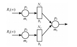
考虑如图 1所示的一个三机装配系统, 其中圆形表示机器, 矩形表示缓冲区.
系统根据以下假设来进行定义:
1) 系统的最终产品(F0)需要两个组件.一个组件(R1)由机器m1处理.我们称系统的这一部分(从机器m1到b1)为零件生产线1.类似地, 另一个组件(R2)由机器m2处理.系统的这一部分(从机器m2到b2)称为零件生产线2.
2) 机器m0从零件生产线1和零件生产线2各取一个完成的零件装配组成一个成品.
3) 机器mi, i=0, 1, 2, 拥有恒定且相同的周期时间τ.以一个加工周期τ为一段, 将时间轴分段.所有机器在一个新的生产批次开始时运行.小批量定制生产下的每个批次具有有限的产量, 每个生产批次的规模为B.每台机器在加工完规定数量的工件后立即停止工作.
4) 机器遵循伯努利可靠性模型, 即, 机器mi, i=0, 1, 2, 如果既没有被阻塞也没有饥饿, 在一个时间间隙(即加工周期)里加工处理一个工件的概率是pi, 未能加工处理一个工件的概率是1-pi.参数pi∈(0, 1)称为机器mi的效率.
5) 每一个在制品缓冲区, bi, i=1, 2, 可以用其容量Ni来表征, 0 < Ni < ∞.
6) 如果机器m0在时间间隙n内处于工作状态, 缓冲区b1或者b2在时间间隙开始时为空, 则机器m0在时隙n内会饥饿.机器m1和m2在一个批次生产结束前不会出现饥饿的情况.
7) 如果机器mi, i=1, 2, 在时间间隙n内处于工作状态, 缓冲区bi在时间间隙开始时有Ni个在制品工件, 并且装配机器m0没能从其中取走一个工件进行处理(由于故障或源自另一条零件生产线的饥饿情况), 则机器mi, i=1, 2, 在时隙n内被阻塞.即, 加工前阻塞机制.同时假设机器m0任何时候都不会被阻塞.
注1.值得注意的是, 在许多生产系统中, 机器周期时间几乎是恒定或接近恒定的.这样的情况大多见于汽车、电子、电器等行业的生产系统.还需注意到, 伯努利可靠性机器模型是适用于平均故障时间接近机器的加工周期的情况(参见使用伯努利模型为实例的文献[22-24]).具有其他可靠性机器模型(例如:几何型、指数型、威布尔型、对数正态型等)的生产系统将在今后的工作中进一步研究.
注2.基于批次的生产广泛用于各种制造系统(小规模, 中等规模, 甚至大规模生产, 单型或多类型产品生产等).一个批次有时被称为一个分组或一个订单.
注3.由于通常定制化生产下每个批次生产数量是有限的, 整个生产过程部分或完全是在暂态下进行的.因此, 严格来说, 稳定状态分析不再适用, 而基于暂态的系统分析是必要的.
注4.上述的模型仅仅包括两条零件生产线和一个装配操作机器.每条零件生产线仅包含了一台机器和一个缓冲区.每条零件生产线拥有多台机器和缓冲区, 以及拥有多条零件生产线的复杂装配系统具有类似的假设, 并且这样的装配系统会在未来工作中进一步研究.
1.2 性能指标
在上述定义的模型框架下, 我们感兴趣的性能指标包括:
1) 生产率PR(n):在时间间隙n+1里, 机器m0生产工件个数的期望;
2) 消耗率CRi(n):在时间间隙n+1里, 机器mi, i=1, 2, 消耗原材料个数的期望;
3) 在制品库存水平, WIPi(n):在时间间隙n里缓冲区bi, i=1, 2, 中的在制品个数的期望;
4) 阻塞率BLi(n):机器mi, i=1, 2, 在时间间隙n+1里被阻塞的概率.
由于机器m0可能由于任意一条零件生产线而饥饿, 我们定义机器饥饿率为:
$ \begin{gathered} S{T_{0,1}}(n) = P[{\mathit{m}_0}在时间间隙n + 1里,由于缓冲区{b_1}为空而饥饿] \hfill \\ S{T_{0,2}}(n) = P[{\mathit{m}_0}在时间间隙n + 1里,由于缓冲区{b_2}为空而饥饿] \hfill \\ \end{gathered} $
一种通过递归聚合来估计这些稳态性能值的方法在文献[22]中被提出.在本文中, 我们提出了在有限量定制生产运行下评估这些暂态性能指标的方法.
此外, 使ct表示机器m0完成生产B个产品的时间.将其均值表示为:
$ \begin{equation} CT = {\rm E}[ct] \end{equation} $
(1) 2. 系统性能精确分析
2.1 性能分析
用fi(n)表示机器mi在时间间隙n结束时已经生产的工件总数量, 用hi(n)表示在时间间隙n结束时缓冲区内的在制品工件数量.显而易见,
$ f_1(n)-f_0(n) = h_1(n) $
$ f_2(n)-f_0(n) =h_2(n) $
那么, 不失一般性, 系统可以用一个状态为(h1(n), h2(n), f0(n))的马尔科夫链来表征, 其中,
$ \begin{array}{l} {h_i}(n) \in \left\{ {0,1, \cdots ,{N_i}} \right\},i = 1,2\\ {f_0}(n) \in \left\{ {0,1, \cdots ,B} \right\} \end{array} $
显然, 此马尔科夫链的最大系统状态数为
$ \begin{equation} \label{equ_Q} Q=(N_1+1)× (N_2+1)× (B+1) \end{equation} $
(2) 需要注意, 有一些系统状态是不可达到的, 比如, (1, 1, B), 因为机器m1和m2在加工好B个工件后立刻停止了运作.换句话说, 在任意一个时间间隙里, h1+f0≤B, 并且h2+f0≤B.
为了计算这一马尔科夫链中的状态间转移概率, 我们首先如表 1排列系统的状态.
表 1 系统状态排序Table 1 Arrangement of the system statesState h1 h2 f0 1 0 0 0 2 0 0 1 ⋮ ⋮ ⋮ ⋮ B+1 0 0 B B+2 0 1 0 B+3 0 1 1 ⋮ ⋮ ⋮ ⋮ Q-1 N1 N2 B-1 Q N1 N2 B 因此, 如果给定任何系统状态S=(h1, h2, f0), 这一状态的序号可通过式(3)计算:
$ \alpha (\mathit{\boldsymbol{S}}) = {h_1}({N_2} + 1)(B + 1) + {h_2}(B + 1) + {f_0} + 1 $
(3) 我们也将状态表示为Sα=(h1α, h2α, f0α).使si(n)=0 (故障), 1 (正常), 表示机器mi在时间间隙n中的状态.根据假设1) ~ 7), 系统的动态特性可以表示为:
$ \begin{gathered} {f_0}(n + 1) = {f_0}(n) + {s_0}(n + 1){\text{min}}\left\{ {{h_1}(n),{h_2}(n),1} \right\} \hfill \\ {h_2}(n + 1) = h_2^\prime (n + 1) + {s_2}(n + 1) \times \hfill \\ \;\;\;\;\;\;\;\;\;\;\;\;\;\;\;{\text{min}}\left\{ {{N_2} - h_2^\prime (n + 1),1} \right\} \hfill \\ {h_1}(n + 1) = h_1^\prime (n + 1) + {s_1}(n + 1) \times \hfill \\ \;\;\;\;\;\;\;\;\;\;\;\;\;\;{\text{min}}\left\{ {{N_1} - h_1^\prime (n + 1),1} \right\} \hfill \\ \end{gathered} $
(4) 其中,
$ \begin{equation*} \begin{split} &h_2^\prime(n+1)=h_2(n)-s_0(n+1) \text{min}\left\{ {h_1(n), h_2(n), 1}\right\}\\ &h_1^\prime(n+1)=h_1(n)-s_0(n+1) \text{min}\left\{{h_1(n), h_2(n), 1}\right\} \end{split} \end{equation*} $
同时也需要注意, 在每个时间间隙中, 系统状态的样本空间是由机器23种的工作状态所组成的.那么,
$ \begin{align} \label{equ_prob} &P[s_1=η_1, s_2=η_2, s_0=η_0]=\nonumber\\ & \prod\limits_{i=0}^{2}p_i^{η_i}(1-p_i)^{1-η_i}, η_i∈\left\{{0, 1}\right\} \end{align} $
(5) 因此, 在每一个时间间隔开始时, 对系统的每一个可达状态i, i∈ {1, ..., Q}, 如果h1i+f0i < B, 并且h2i+f0i < B, 可以枚举所有的23种机器状态的组合, 根据系统动态性式(4)来确定相应的在这一时间间隔结束时的结果状态j, j∈{1, ..., Q}.然后, 对于得到相同结果状态的机器状态组合情况, 使用式(5)来计算相应的转移概率, 并将这些概率相加, 最终得到一个时间间隔里, 从起始的系统状态i到结果状态j的转移概率.对于所有符合条件的系统状态重复这一步骤.
然后, 对于h1i+f0i=B, 或者h2i+f0i=B, 系统状态之间的转移概率如下:
$ \begin{gathered} P[{h_1}(n + 1) = i - 1, {h_2}(n + 1) = j - 1, {f_0}(n + 1) = \hfill \\ \;\;\;k + 1|{h_1}(n) = i, {h_2}(n) = j, {f_0}(n) = k] = \hfill \\ \;\;\;(1 - {p_1}){p_0}, \;i \in \left\{ {1, ..., {N_1}} \right\}, \;j \in \left\{ {1, ..., {N_2}} \right\}, \hfill \\ \;\;\;k \in \left\{ {0, ..., B - 1} \right\}, {\text{且}}\;i + k < B, \;j + k = B \hfill \\ \end{gathered} $
$ \begin{gathered} P[{h_1}(n + 1) = i, {h_2}(n + 1) = j - 1, {f_0}(n + 1) = \hfill \\ \;\;\;k + 1|{h_1}(n) = i, {h_2}(n) = j, {f_0}(n) = k] = {p_1}{p_0}, \hfill \\ \;\;\;i \in \left\{ {1, ..., {N_1}} \right\}, \;j \in \left\{ {1, ..., {N_2}} \right\}, \hfill \\ \;\;\;k \in \left\{ {0, ..., B - 1} \right\}, {\text{且}}i + k < B, j + k = B \hfill \\ \end{gathered} $
$ \begin{gathered} P[{h_1}(n + 1) = i - 1, {h_2}(n + 1) = j - 1, {f_0}(n + 1) = \hfill \\ \;\;\;k + 1|{h_1}(n) = i, {h_2}(n) = j, {f_0}(n) = k] = \hfill \\ \;\;\;\left( {1 - {p_2}} \right){p_0}, \;i \in \left\{ {1, ..., {N_1}} \right\}, \;j \in \left\{ {1, ..., {N_2}} \right\}, \hfill \\ \;\;\;k \in \left\{ {0, ..., B - 1} \right\}, {\text{且}}\;i + k = B, \;j + k < B \hfill \\ \end{gathered} $
$ \begin{gathered} P[{h_1}(n + 1) = i - 1, {h_2}(n + 1) = j, {f_0}(n + 1) = \hfill \\ \;\;\;k + 1|{h_1}(n) = i, {h_2}(n) = j, {f_0}(n) = k] = {p_2}{p_0}, \hfill \\ \;\;\;i \in \{ 1, ..., {N_1}\} , \;j \in \{ 1, ..., {N_2}\} , \hfill \\ \;\;\;k \in \{ 0, ..., B - 1\} , {\text{且}}\;i + k = B, \;j + k < B \hfill \\ \end{gathered} $
$ \begin{gathered} P[{h_1}(n + 1) = i, {h_2}(n + 1) = j, {f_0}(n + 1) = k| \hfill \\ \;\;\;{h_1}(n) = i, {h_2}(n) = j, {f_0}(n) = k] = \hfill \\ \;\;\;(1 - {p_1})(1 - {p_2})(1 - {p_0}), \hfill \\ \;\;\;i \in \{ 1, ..., {N_1}\} , \;j \in \{ 1, ..., {N_2}\} , \hfill \\ \;\;\;k \in \{ 0, ..., B - 1\} , {\text{且}}\;i + k = B, \;j + k < B \hfill \\ \end{gathered} $
$ \begin{gathered} P[{h_1}(n + 1) = i, {h_2}(n + 1) = j, {f_0}(n + 1) = k| \hfill \\ \;\;\;{h_1}(n) = i, {h_2}(n) = j, {f_0}(n) = k] = \hfill \\ \;\;\;(1 - {p_1})(1 - {p_2})(1 - {p_0}), \hfill \\ \;\;\;i \in \{ 1, ..., {N_1}\} , j \in \{{ 1, ..., {N_2}\}} , \hfill \\ \;\;\;k \in \{{ 0, ..., B - 1\}} , {\text{且}}\;i + k < B, \;j + k = B \hfill \\ \end{gathered} $
$ \begin{gathered} P[{h_1}(n + 1) = i, {h_2}(n + 1) = j, {f_0}(n + 1) = k| \hfill \\ \;\;\;{h_1}(n) = i, {h_2}(n) = j, {f_0}(n) = k] = {p_1}{p_2}{p_0}, \hfill \\ \;\;\;i \in \{ 1, ..., {N_1}\} , j \in \{ 1, ..., {N_2}\} , \hfill \\ \;\;\;k \in \left\{ {0, ..., B - 1} \right\}, 且\;i + k = B, \;j + k < B \hfill \\ \end{gathered} $
$ \begin{gathered} P[{h_1}(n + 1) = i, {h_2}(n + 1) = j, {f_0}(n + 1) = k + 1| \hfill \\ \;\;\;{h_1}(n) = i, {h_2}(n) = j, {f_0}(n) = k] = {p_1}{p_2}{p_0}, \hfill \\ \;\;\;i \in \left\{ {1, ..., {N_1}} \right\}, j \in \left\{ {1, ..., {N_2}} \right\}, \hfill \\ \;\;\;k \in \left\{ {0, ..., B - 1} \right\}, {\text{且}}\;i + k < B, j + k = B \hfill \\ P[{h_1}(n + 1) = i - 1, {h_2}(n + 1) = j - 1, {f_0}(n + 1) = \hfill \\ \;\;\;k + 1|{h_1}(n) = i, {h_2}(n) = j, {f_0}(n) = k] = {p_0}, \hfill \\ \end{gathered} $
$ \begin{gathered} \;\;\;i \in\left\{ 1, ..., {N_1}\right\}, \;j \in \left\{1, ..., {N_2}\right\}, \hfill \\ \;\;\;k \in\left\{ 0, ..., B - 1\right\}, {\text{且}}\;i + k = B, \hfill \\ \end{gathered} $
$ \begin{gathered} P[{h_1}(n + 1) = i, {h_2}(n + 1) = j, {f_0}(n + 1) = k| \hfill \\ \;\;\;{h_1}(n) = i, {h_2}(n) = j, {f_0}(n) = k] = 1 - {p_0}, \hfill \\ \;\;\;i \in \left\{1, ..., {N_1}\right\}, \;j \in \left\{1, ..., {N_2}\right\}, \hfill \\ \;\;\;k \in \left\{0, ..., B - 1\right\}, {\text{且}}\;i + k = B, j + k = B \hfill \\ \end{gathered} $
$ \begin{gathered} P[{h_1}(n + 1) = 0, {h_2}(n + 1) = 0, {f_0}(n + 1) = \hfill \\ B|\;{h_1}(n) = 0, {h_2}(n) = 0, {f_0}(n) = B] = 1 \hfill \\ \end{gathered} $
(6) 用x(n)=[x1(n)... xQ(n)]T, 其中xi(n)表示系统在状态i的概率, 并且用A表示转移状态矩阵.那么, 系统状态进化可表示为:
$ \begin{equation} \begin{split} {\boldsymbol{x}}(n+1)=A{\boldsymbol{x}}(n), {\boldsymbol{x}}(0)=[1~ 0~ ...~ 0]^\textrm{T} \end{split} \end{equation} $
(7) 系统的实时性能可以通过下式计算:
$ \begin{equation} \label{equ_exac} \begin{split} PR(n)= {{\boldsymbol{V}}}_1{\boldsymbol{x}}(n), \\ CR_i(n)= {{\boldsymbol{V}}}_{2, i}{\boldsymbol{x}}(n), \ i=1, 2\\ WIP_i(n)={{\boldsymbol{V}}}_{3, i}{\boldsymbol{x}}(n), \ i=1, 2\\ BL_i(n)= {{\boldsymbol{V}}}_{4, i}{\boldsymbol{x}}(n), \ i=1, 2\\ ST_{0, i}(n)= {{\boldsymbol{V}}}_{5, i}{\boldsymbol{x}}(n), \ i=1, 2\\ CT= {{\boldsymbol{V}}}_6{\boldsymbol{x}}(n) \end{split} \end{equation} $
(8) 其中
$ {{\boldsymbol{V}}}_1=[0_{1, (N_2+1)(B+1)}\;\;\;[0_{1, B+1} [p_0J_{1, B}\;\;\;0]\\ \;\;\;C_{(B+1)× N_2(B+1)}] C_{(N_2+1)(B+1)× N_1(N_2+1)(B+1)}]\\ {{\boldsymbol{V}}}_{2, 1}=[p_1J_{1, N_1(N_2+1)(B+1)}\ 0_{1, B+1}\ p_1p_0J_{1, N_2(B+1)}]\\ {{\boldsymbol{V}}}_{2, 2}=[p_1J_{1, N_2(B+1)}\;\;\; 0_{1, B+1}\;\;\;[p_2J_{1, N_2(B+1) }\\ \;\;\; p_2p_0p_1J_{1, B+1}]C_{(N_2+1)(B+1)× N_1(N_2+1)(B+1)}]\\ {{\boldsymbol{V}}}_{3, 1}=[0_{1, B+1}\;\;\;1× J_{1, B+1} { ...} N_2× J_{1, B+1}] \\ \;\;\;C_{(N_2+1)(B+1)× Q}\\ {{\boldsymbol{V}}}_{3, 2}=[0_{1, (N_2+1)(B+1)}\;\;\;1× J_{1, (N_2+1)(B+1)} \\ \;\;\; N_1× J_{1, (N_2+1)(B+1)}]\\ {{\boldsymbol{V}}}_{4, 1}=[0_{1, N_1(N_2+1)(B+1)}\;\; p_1J_{1, B+1}\\ \;\;\; p_1(1-p_0)J_{1, N_2(B+1)}]\\ {{\boldsymbol{V}}}_{4, 2}=[0_{1, N_2(B+1)} \;\;\; p_2J_{1, B+1}\;\;\; [0_{1, N_2(B+1)}\\ \;\;\; p_2(1-p_0)J_{1, B+1}] C_{(N_2+1)(B+1)× N_1(N_2+1)(B+1)}]\\ {{\boldsymbol{V}}}_{5, 1}=[p_0J_{1, (N_2+1)(B+1)} \;\;\;0_{1, N_1(N_2+1)(B+1)}]\\ {{\boldsymbol{V}}}_{5, 2}=[p_0J_{1, B+1} \;\;\;0_{1, N_2(B+1)}] C_{(N_2+1)(B+1)× Q}\\ {{\boldsymbol{V}}}_6=[0_{1, (N_2+1)(B+1)+2B}\; p_0 \; 0 { ...} 0] $
其中, 01, k和J1, k分别代表 1× k的零矩阵和元素全为1的矩阵.与此同时, i× j维矩阵Ci× j=[Ii~...~ Ii]表示由j/i个单位矩阵Ii组成的矩阵.
3. 基于分解的性能评估
上面描述的精确分析可以扩展到更大的系统, 即每个零件生产线中有多台机器的系统.然而, 随着机器数量M, 缓冲区容量Ni's, 和生产规模B的增长, 马尔科夫链状态的数量呈指数型增长, 这将导致对大型的复杂装配系统的分析变得不可能.因此, 本节提出了一种基于分解的算法, 并将其应用于三台伯努利机器的小型装配系统.相应的研究结果将在未来的工作中扩展到更通用的大型系统中.
3.1 基于分解的概念
文献[8]提出一种分解方法, 将原系统分解为一对串行线:上线和下线, 研究了基于无限原材料供应的装配系统的稳态性能.此外, 我们以前的工作[20-21]解决了这类系统的暂态性能研究的问题.与此同时, 当考虑到小批量有限量生产运行下的串行线, 基于暂态的系统性能近似评估也在我们以前的工作[16-17]中进行了讨论.在这一节中, 我们将基于有限量生产运行下系统的暂态性能分析扩展到三台机器的装配系统性能分析研究中.对由多台机器组成的零件生产线或多条零件生产线以及多个装配操作的复杂装配系统, 将在今后的研究中进行分析.
具体而言, 引入三种辅助系统/生产线来分析此类系统.辅助装配系统(图 2所示)首先被引入, 这一辅助装配系统具有所有原始的机器和缓冲区, 但假设具有无限的原材料供应.
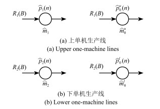
为了研究这一辅助装配系统的暂态性能, 分析方法可以参考我们以前的工作(参阅文献[20]).具体而言, 使用辅助两机线(图 3)来近似分析.
上生产线通过移除辅助装配系统中的机器m2和缓冲区b2来构造.考虑到这种修改, 组装机器m0由效率p0u(n)随时间变化的虚拟机器m0u (图 3 (a))来代替.同样, 下生产线可以通过移除机器m1和缓冲区b1, 同时使用效率p0l(n)随时间变化的虚拟机器m0l来构造.
为了获得p0u(n)和p0l(n), 注意, 上生产线中的虚拟机器m0u, 只有原来的装配操作中装配机器m0处于工作状态并且缓冲区b2非空的情况下, 才可能处于工作状态.同样, 下生产线中的虚拟机器m0l, 只有原来的装配操作中装配机器m0处于工作状态并且缓冲区b1非空的情况下, 才可能处于工作状态.因此, 让hi(n)表示在时间间隙n结束时缓冲区bi中的在制品零件数, p0u(n)和p0l(n)可以通过式(9)估算:
$ \begin{split} p_{0}^u(n) &≈ p_{0}\left (1-P[h_{2}(n-1)=0]\right )\\ p_{0}^l(n) &≈ p_{0}\left (1-P[h_{1}(n-1)=0]\right ) \end{split} $
(9) 用于分析这种辅助两机串行线的方法在文献[11]中被提出.具体来说, 用xh, iu(n)和xh, il(n), 分别来表示辅助两机生产线中b1和b2在时隙n结束时, 有i个工件的概率.令xhu(n)=[xh, 0u(n)\...\ xh, N1u(n)]T, xhl(n)=[xh, 0l(n)\...\ xh, N2l(n)]T.根据文献[11], xhu(n)的演化可表示为:
$ \begin{gathered} \mathit{\boldsymbol{x}}_h^u(n + 1) = A_2^u(n)\mathit{\boldsymbol{x}}_h^u(n),\;\;\sum\limits_{i = 0}^{{N_1}} {x_{h,\mathit{i}}^u(n) = 1} \hfill \\ x_{h,i}^u(0) = \left\{ \begin{gathered} 1,\;\;\;\;i = 0 \hfill \\ 0,\;\;\;\;其他 \hfill \\ \end{gathered} \right. \hfill \\ \end{gathered} $
(10) 其中, A2u(n)在式(11)中进行了定义.同时, xhl(n)和A2l(n)可以通过同样的方法被推导出来.
最后, 引入有限量生产运行下的辅助单机生产线(见图 4).
$ \begin{equation} A_2^u(n)=\left [ \begin{array}{cccccc} 1-p_1&p_0^u(1-p_1)&0&{ ...}&0\\ p_1&1-p_1-p_0^u+2p_1p_0^u&p_0^u(1-p_1) &{ ...}&0\\ 0&p_1(1-p_0^u)&\ddots& \ddots&\vdots\\ \vdots&\vdots&\ddots &1-p_1-p_0^u+2p_1p_0^u&p_0^u(1-p_1)\\ 0&0&{ ...}&p_1(1-p_0^u)&p_1p_0^u+1-p_0^u \end{array} \right ] \label{eqn_A2u_matrix} \end{equation} $
(11) 由于无论是m1还是m2, 能够生产一个工件的前提条件都是当且仅当它处于工作状态且不被阻塞, 同时无论m0u或者是m0l, 能够生产的条件是当且仅当其处于工作状态且不会饥饿, 我们定义随时间变化的辅助单机机器效率如下:
$ \begin{equation} \label{equ_auxi_1m} \begin{split} \widehat{p}_1(n)= &p_1[1-x_{h, N_1}^u(n-1)(1-p_0^u(n))]\\ \widehat{p}_2(n)= &p_2[1-x_{h, N_2}^l(n-1)(1-p_0^l(n))]\\ \widehat{p}_0^u(n)= &p_0^u(n)[1-x_{h, 0}^u(n-1)]\\ \widehat{p}_0^l(n)= &p_0^l(n)[1-x_{h, 0}^l(n-1)] \end{split} \end{equation} $
(12) 换句话说, 辅助单机生产线中的机器, ,当且仅当机器m1和m2处于工作状态, 并且辅助两机生产线上的第一台机器在同一时隙期间不会被阻塞的情况下, 才可以处理工件.同样, 辅助单机生产线中的机器$\widehat m_0^u $, $\widehat m_0^l $当且仅当机器m0u和m0l处于工作状态, 并且辅助两机生产线上的第二台机器在同一时隙期间不会被饥饿的情况下, 才可以处理工件.
为了分析辅助单机生产线, 注意, 它们每个都可由一个马尔科夫链来表征, 其中, 系统状态为已被这台机器加工过的工件数量(参阅文献[17]).让xf(i)(n)=[xf, 0(i)(n)\ xf, 1(i)(n)... xf, B(i)(n)]T, 其中xf, j(i)(n)表示$ {\widehat m_1}$, i=1, 2, 在时隙n结束时已经加工了j个工件的概率. xf(i)(n)的演化可以通过以下线性时变方程给出:
$ \begin{equation} \label{equ_evolu_b} \begin{split} {\boldsymbol{x}}_f^{(i)}(n+1)=A_{f}^{(i)}(n){\boldsymbol{x}}_f^{(i)}(n)% \sum\limits_{i=0}^{B}x_i(n)=1, \end{split} \end{equation} $
(13) 其中初始状态是
$ \begin{equation*} {\boldsymbol{x}}_f^{(i)}(0)=[1\ 0\ ...\ 0\ 0]^\textrm{T} \end{equation*} $
时变的转移矩阵Af(i)(n)可以通过下式计算:
$ \begin{equation} \label{equ_af_matrix} A_f^{(i)}(n) = \left [ \begin{array}{cccc} 1-\widehat{p}_i(n)&\\ \widehat{p}_i(n)&\ddots \\ &\ddots&1-\widehat{p}_i(n)\\ &&\widehat{p}_i(n)&1\\ \end{array} \right ] \end{equation} $
(14) 其中${\widehat p_i} $(n)通过式(12)来计算.
此外, 为了分析虚拟机器$\widehat m_0^u $和$\widehat m_0^l $, 使xf(0, u)(n)=[xf, 0(0, u)(n)\ xf, 1(0, u)(n)\...\ xf, B(0, u)(n)]T, 并且xf(0, l)(n)=[xf, 0(0, l)(n)\ xf, 1(0, l)(n)\...\ xf, B(0, l)(n)]T, 其中xf, j(0, u)(n)和xf, j(0, l)(n)分别表示机器$\widehat m_0^u $和$\widehat m_0^l $, 在时隙n结束时已经生产加工j个工件的概率.类似的分析同样适用, xf(0, u)(n)和xf(0, l)(n)的演化将由以下线性时变方程给出:
$ \begin{gathered} \mathit{\boldsymbol{x}}_f^{(0,u)}(n + 1) = A_f^{(0,u)}(n)\mathit{\boldsymbol{x}}_f^{(0,u)}(n) \hfill \\ \mathit{\boldsymbol{x}}_f^{(0,l)}(n + 1) = A_f^{(0,l)}(n)\mathit{\boldsymbol{x}}_f^{(0,l)}(n) \hfill \\ \end{gathered} $
(15) 其中初始状态是
$ \mathit{\boldsymbol{x}}_f^{(0,u)}(0) = {[1\;0\;...0]^{\text{T}}},{\text{ }}\mathit{\boldsymbol{x}}_f^{(0,l)}(0) = {[1\;0...\;0]^{\text{T}}} $
时变转移状态矩阵Af(0, u)(n)可以通过式(16)来计算:
$ A_f^{(0,u)}(n) = \left[ {\begin{array}{*{20}{c}} {1 - \hat p_0^u(n)}&{}&{}&{} \\ {\hat p_0^u(n)}& \ddots &{}&{} \\ {}& \ddots &{1 - \hat p_0^u(n)}&{} \\ {}&{}&{\hat p_0^u(n)}&1 \end{array}} \right] $
(16) 其中通过式(12)来计算. Af(0, l)(n)可以通过相同的方法进行推导, 并把所有(16)中的${\hat p_0^u(n)} $用通过(12)计算得来的来替代.
综上, 为了分析图 1中的有限量运行下的三机装配线的暂态性能, 我们将原始系统的动态特性进行分解和简化, 通过分析一系列分解后相互影响的动态特性更加简单的系统, 来近似评估原始系统的实时性能.具体来说, 对于原始系统(图 1), 其动态特性包括两方面:缓冲区中在制品数量的演化和在每台机器上已完成加工处理的工件数量.首先引入使用原始系统机器和缓冲区参数的辅助装配系统, 同时假设无限原材料(图 2).在这个系统中, 我们只关注系统中的缓冲区在制品数量的演化.为了分析图 2所示系统, 进一步引入辅助双机串行线(图 3), 其中, 为了考虑移除相应机器和缓冲区所带来的影响, 上生产线和下生产线中装配机器所在位置分别使用相应的参数时变的虚拟机器来替代.因此, 通过分析辅助双机串行线(图 3), 事实上可以得到辅助装配系统(图 2)中系统状态(缓冲区在制品数量)的实时分布情况.最后, 引入辅助单机生产线(图 4)来分析在相应机器上完成加工处理工件数量的动态特性.而每一台单机生产线的时变参数都是在考虑了辅助双机串行线中的系统状态的影响下, 近似推导得出的.
3.2 性能评估近似公式
基于上述构造的辅助生产线或生产系统, 我们提出了近似原系统性能指标的计算公式.首先, 有限量生产运行下一个批次的生产完成时间通过使用辅助虚拟单机线$\widehat m_0^u $或$\widehat m_0^l $中的任意一个来近似估算.不失一般性, 使用$\widehat m_0^u $, 同时令${{\hat p}_{ct}}(n)$表示原始系统中机器m0在时隙n结束时处理加工完整个批次所有工件的近似概率.那么,
$ {\hat P_{ct}}(n) = P[\left\{ {\mathit{\widehat m}_0^u在时隙\;\mathit{n}\;处于工作状态} \right\} \cap \{ 已加工处理完\mathit{B} - 1个工件\} ] = \hat p_0^u(n)x_{f,B - 1}^{(0,u)}(n - 1) $
(17) 其次, 原系统的生产率和各个零件生产线的消耗率可由辅助单机生产线的生产率来近似:
$ \begin{equation} \label{equ_perfor_appr} \begin{split} \widehat{PR}(n)= &[\widehat{p}_0^u(n)J_{1, B} 0]{\boldsymbol{x}}_{f}^{(0, u)}(n-1)\\ \widehat{CR}_1(n)= &[\widehat{p}_1(n)J_{1, B} 0]{\boldsymbol{x}}_{f}^{(1)}(n-1)\\ \widehat{CR}_2(n)= &[\widehat{p}_2(n)J_{1, B} 0]{\boldsymbol{x}}_{f}^{(2)}(n-1) \end{split} \end{equation} $
(18) 为了估算WIPi(n), BLi(n)和ST0, i(n), 两种辅助生产线需要结合起来.具体来说, 这些性能评估使用相应的辅助两机生产线来近似估算, 同时考虑相对应的机器在辅助单机生产线上还没有完成加工整个批次所有产品的概率:
$ \begin{align} \label{equ_appro_2M_perfor} \widehat{WIP}_1(n)= &[0\ 1\ { ...}\ N_1] {\boldsymbol{x}}_{h}^{u}(n)(1-x_{f, B}^{(0, u)}(n-1))\nonumber\\ \widehat{WIP}_2(n)= &[0\ 1\ { ...}\ N_2] {\boldsymbol{x}}_{h}^{l}(n)(1-x_{f, B}^{(0, l)}(n-1))\nonumber\\ \widehat{ST}_{0, 1}(n)= &[p_0 0_{1, N_1}] {\boldsymbol{x}}_{h}^{u}(n-1)(1-x_{f, B}^{(0, u)}(n-1))\nonumber\\ \widehat{ST}_{0, 2}(n)= &[p_0 0_{1, N_2}] {\boldsymbol{x}}_{h}^{l}(n-1)(1-x_{f, B}^{(0, l)}(n-1))\nonumber\\ \widehat{BL}_1(n)= &[{0}_{1, N_1} p_1(1-p_2)] {\boldsymbol{x}}_{h}^u(n-1)×\nonumber\\ &(1-x_{f, B}^{(1)}(n-1))\nonumber\\ \widehat{BL}_2(n)= &[{0}_{1, N_2} p_2(1-p_2)] {\boldsymbol{x}}_{h}^l(n-1)×\nonumber\\ & (1-x_{f, B}^{(2)}(n-1)) \end{align} $
(19) 最后, 一个批次的完成时间期望可以被近似为:
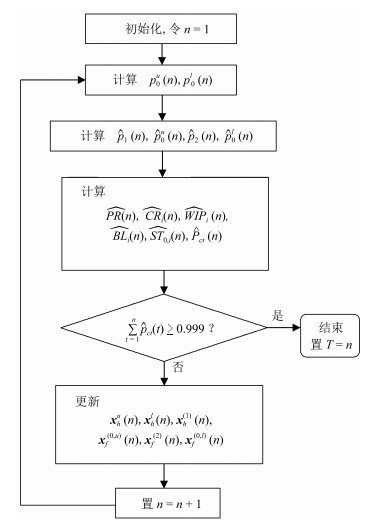
$ \begin{equation} \label{equ_CT} \begin{split} \widehat{CT}& = \sum\limits_{n=1}^T n\widehat{P}_{ct}(n) \\ \end{split} \end{equation} $
(20) 其中, T满足以下条件:
$ \begin{equation*} \sum\limits_{n=1}^T\widehat{P}_{ct}(n)\geq0.999 \end{equation*} $
综上, 基于分解的计算方法流程图如图 5所示.
对于所提出的性能近似的方法的精确程度, 我们通过对10 000条参数随机而均匀地从式(21)所示的集合或者区间中选取的三机伯努利装配系统, 进行基于精确解析和基于分解的近似性能评估分析, 来验证所提近似方法的精确性.
$ \begin{align} \label{equ_para} B&∈\left\{{20, 21, { ...}, 100}\right\}, \ p_i∈(0.7, 1), \ i=0, 1, 2\nonumber\\ N_i&∈\left\{{2, 3, 4, 5}\right\}, \ i=1, 2 \end{align} $
(21) 对于每一条参数随机产生的装配系统, 我们分别通过精确分析式(8)和基于分解的近似分析式(17) ~ (20)来计算其各项性能指标.结果显示, 对于这10 000条装配系统的各项性能指标的平均相对误差, 它们的中值都在1 %以下.
作为一个例子, 考虑图 6所显示的装配系统.每个机器(圆形表示)上的数字表示其效率, 而每个缓冲区(矩形)中的数字表示其容量.这些参数是随机生成的.在本例中, 所有缓冲区都被假设在起始状态时是空的.首先需要注意的是, 使用精确分析方法, 根据式(\ref{equ_Q), 系统的状态数量为1 620;而经过分解后, 我们只需要分析六个相对较小但相互影响的系统:一条双机上生产线, 一条双机下生产线, 两条上单机生产线, 两条下单机生产线.六个较小的马尔科夫链的总状态数为333.在保证精确度的基础上, 相较精确分析, 基于分解的近似分析使系统状态数量有了极大的降低.与此同时, 从计算时间的角度来看, 使用MATLAB软件在同一台电脑配置为因特尔酷睿i7-6700的CPU和16 GB的RAM上, 基于精确分析和基于分解的近似分析, 所需要的运算时间分别为13.35秒和0.11秒, 近似算法在计算高效性上也显示出了极大的优势.系统的暂态性能如图 7所示, 从图中可以看出, 整个生产运行过程分为三个阶段.在第一阶段, 产品开始进入空系统.在此期间, 生产率和在制品数量都从0上升到稳态值.同时, 由于更多的工件进入系统, 零件生产线1 (或者零件生产线2)的消耗率从p1 (或者p2)开始逐渐减小.在第二阶段中, 系统运行接近稳定状态, 所有暂态性能指标都或多或少地处于平稳状态.最后, 当生产运行接近完成时, 所有性能指标开始下降, 最终达到0.基于该分解算法的高精度也可以从图中清晰地看到.需要注意的是, 虽然精确的分析在这种小型装配系统中仍然可以被推导出来, 然而随着系统参数(M, Ni's和B)的增长, 精确分析也变得越来越不可能实现.基于分解思想的性能近似评估方法的计算高效性将在这样的大型装配系统中体现出来.深入的相关研究将在未来的工作中被进一步讨论.
4. 结束语
本文研究了具有三台伯努利机器, 有限缓冲区容量和有限量生产运行下的装配系统的暂态性能评估问题.具体地, 首先推导了系统性能评价的精确数学模型和解析公式.然后, 提出了一种基于分解的性能评估算法, 通过将系统转换成一系列相互作用的辅助串行线来近似评估原始系统的暂态性能.论文推导了基于分解的三机装配系统实时性能估计公式, 并通过数值实验验证了算法的准确性和计算高效性.
 图 7 分解近似与精确分析的三机伯努利装配系统暂态实时性能评估对比Fig. 7 Comparison of decomposition-based approxiamtion and exact analysis for transient performance evaluation in assembly system with three Bernoulli machines
今后在这方面的工作包括将算法扩展到每个零件生产线具有多台机器和多个缓冲区的系统, 或多条零件生产线和多装配操作的复杂装配系统.此外, 还会将研究结果推广到具有其他机器可靠性模型(几何型、指数型、威布尔型等)的装配系统中.
-
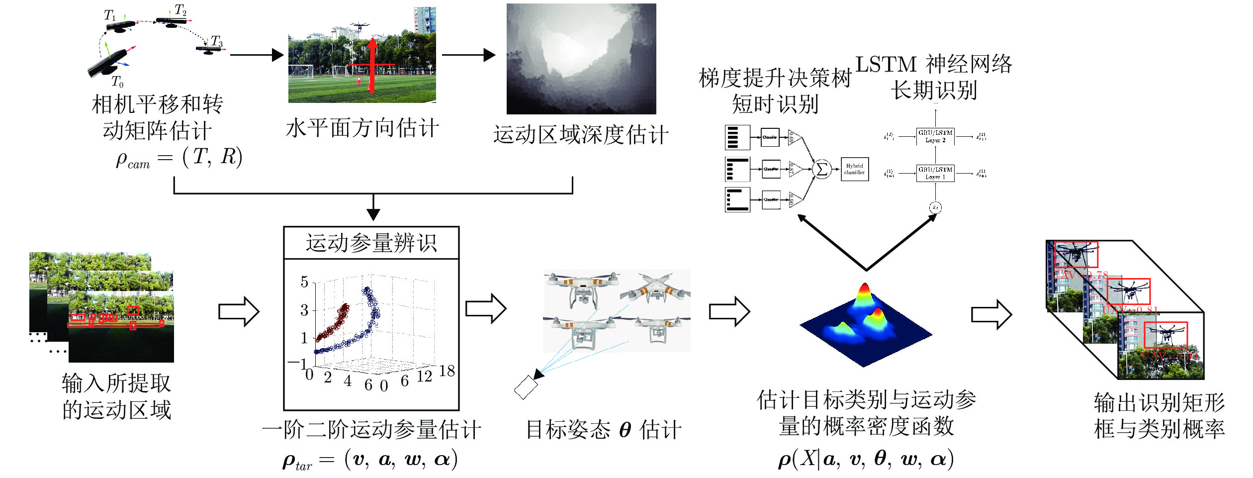
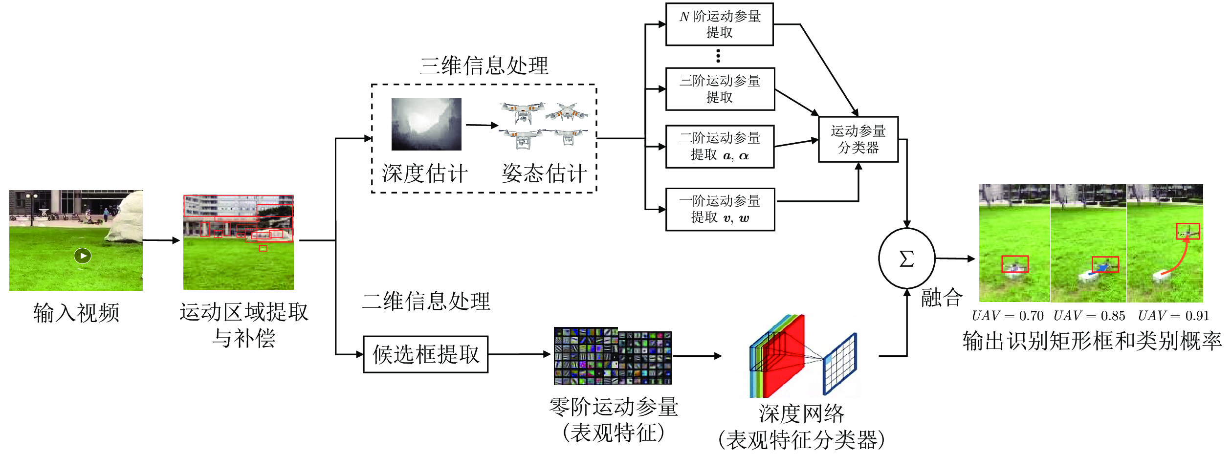
图 2 基于多阶运动参量的目标识别方法流程图(MoKiP)
Fig. 2 Flowchart of multi-order kinematic parameters based detection method (MoKiP)
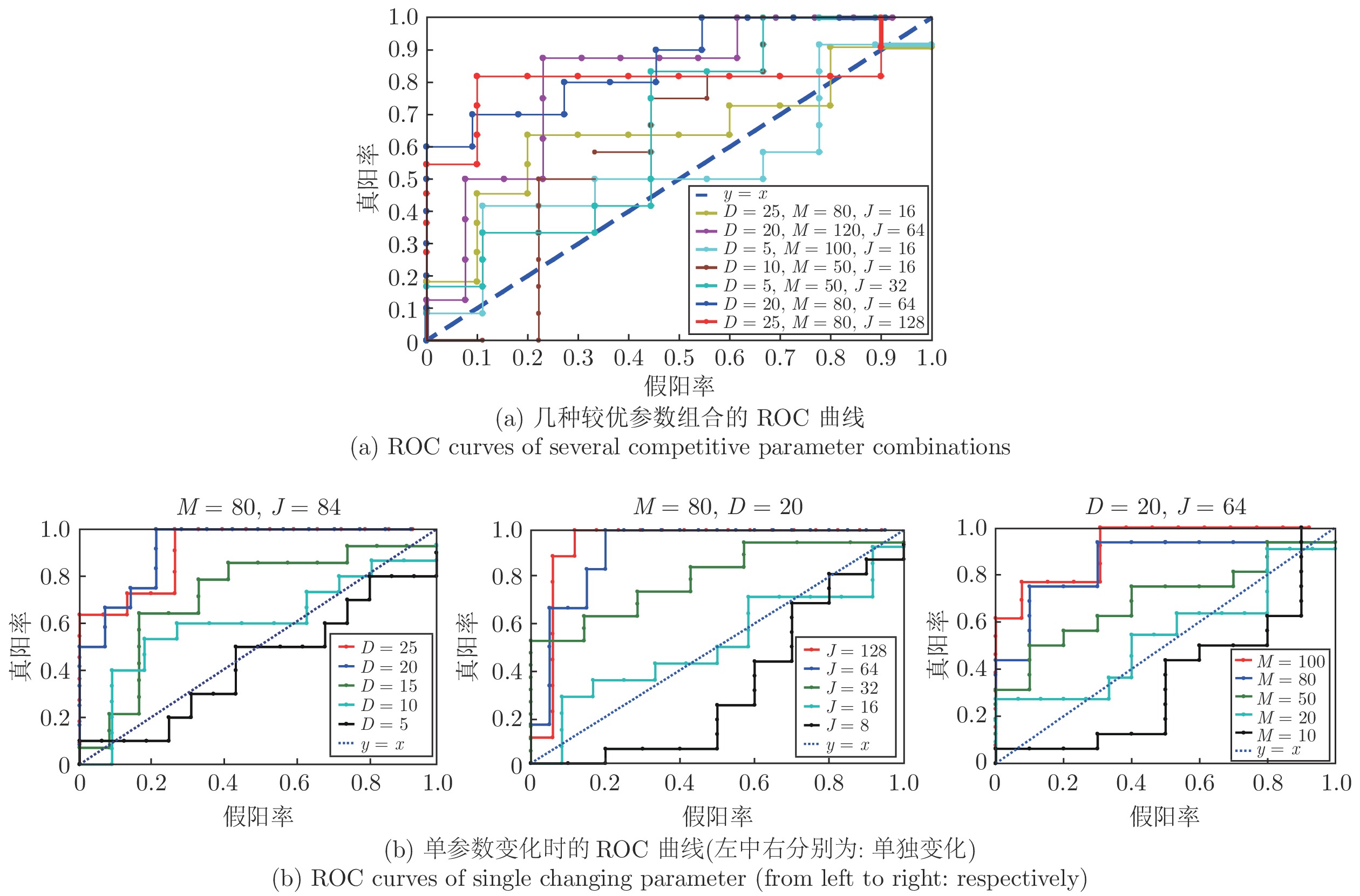
图 8 不同参数组合的ROC曲线单参数变化时的ROC曲线(左中右分别为
$D、M、J$ 单独变化)Fig. 8 ROC curves of different GBDT parameter combinations (The subplots from left to right are corresponding to D、M、J respectivly)
表 2 MUD数据集采集设备说明
Table 2 Main equipment for acquisition of multi-scale UAV dataset (MUD)
设备 参数 精度 相机 SONY A7 ILCE-7M2, $6\,000 \times 4\,000$像素FE 24 ~ 240 mm, F 3.5 ~ 6.3 — GPS GPS/GLONASS双模 垂直$\pm 0.5\;{\rm{m} },$ 水平$ \pm 1.5\;{\rm{m}}$ 激光测距仪 SKIL Xact 0530, 0 ~ 80 m $ \pm 0.2\;{\rm{mm}}$  下载: 导出CSV
表 4 不同深度估计方法误差对比
Table 4 Error of different depth estimation methods
方法 探测范围 绝对误差 平方误差 均方根误差 $\delta < 1.25$ $\delta < {1.25^2}$ $\delta < {1.25^3}$ DORN[51] 0 ~ 100 m 0.103 0.321 9.014 0.832 0.875 0.922 GeoNet[63] 0 ~ 100 m 0.280 2.813 14.312 0.817 0.849 0.895 双目视觉[64] 0 ~ 100 m 0.062 1.210 0.821 0.573 0.642 0.692 激光测距 0 ~ 200 m 0.041 2.452 1.206 0.875 0.932 0.961 DORN[51] 200 ~ 500 m 0.216 1.152 13.021 0.672 0.711 0.748 GeoNet[63] 200 ~ 500 m 0.398 5.813 18.312 0.617 0.649 0.696 双目视觉[64] 200 ~ 500 m 0.786 5.210 25.821 0.493 0.532 0.562 激光测距 200 ~ 500 m 0.078 3.152 2.611 0.891 0.918 0.935
下载: 导出CSV
参数 说明 ${\boldsymbol v}$ 速度 ${\boldsymbol a}$ 加速度 ${\boldsymbol \omega}$ 角速度 ${\boldsymbol \alpha }$ 角加速度 X 轴分量方向 与图像平面坐标系中 u 轴方向保持一致 Y 轴分量方向 与图像平面坐标系中 v 轴方向保持一致 Z 轴分量方向 铅垂向上
下载: 导出CSV
表 6 运动参量的决策树模型识别结果混淆矩阵
Table 6 Confusion matrix of MokiP by using GDBT
真实值
预测值旋翼无人机 鸟类 行人 车辆 其他物体 旋翼无人机 0.67 0.25 0.02 0.01 0.12 鸟类 0.21 0.58 0.01 0.00 0.10 行人 0.01 0.02 0.75 0.06 0.09 车辆 0.01 0.00 0.10 0.80 0.08 其他物体 0.10 0.15 0.12 0.13 0.61
下载: 导出CSV
表 7 不同识别方法性能指标对比表
Table 7 Comparison of performance indexes for different detection method
下载: 导出CSV
表 8 运动参量的性质对无人机识别的影响表
Table 8 Impact of the parameter properties on UAV detection
参量贡献度$D$ 平动参量 旋转参量 总贡献度 一阶参量 7.2% 20.1% 27.3% 二阶参量 34.1% 38.6% 72.7% 总贡献度 41.3% 58.7% 1
下载: 导出CSV
表 9 运动参量的方向对无人机识别的影响表
Table 9 Impact of the parameter direction on UAV detection
参量贡献度$D$ 沿 X 轴方向 沿 Y 轴方向 沿 Z 轴方向 总贡献度 平动参量 8.3% 8.8% 24.2% 41.3% 旋转参量 18.7% 18.8% 22.2% 58.7% 总贡献度 27.0% 27.6% 46.4% 1
下载: 导出CSV
-
[1] 李菠, 孟立凡, 李晶, 刘春美, 黄广炎. 低空慢速小目标探测与定位技术研究. 中国测试, 2016, 42(12): 64-69 doi: 10.11857/j.issn.1674-5124.2016.12.014Li Bo, Meng Li-Fan, Li Jing, Liu Chun-Mei, Huang Guang-Yan. Research on detecting and locating technology of LSS-UAV. China Measurement & Test, 2016, 42(12): 64-69 doi: 10.11857/j.issn.1674-5124.2016.12.014 [2] Wang Z H, Lin X P, Xiang X Y, Blasch E, Pham K, Chen G S, et al. An airborne low SWaP-C UAS sense and avoid system. In: Proceedings of SPIE 9838, Sensors and Systems for Space Applications IX. Baltimore, USA: SPIE, 2016. 98380C [3] Busset J, Perrodin F, Wellig P, Ott B, Heutschi K, Rühl T, et al. Detection and tracking of drones using advanced acoustic cameras. In: Proceedings of SPIE 9647, Unmanned/Unattended Sensors and Sensor Networks XI; and Advanced Free-Space Optical Communication Techniques and Applications. Toulouse, France: SPIE, 2015. 96470F [4] Mezei J, Fiaska V, Molnár A. Drone sound detection. In: Proceedings of the 16th IEEE International Symposium on Computational Intelligence and Informatics (CINTI). Budapest, Hungary: IEEE, 2015. 333−338 [5] 张号逵, 李映, 姜晔楠. 深度学习在高光谱图像分类领域的研究现状与展望. 自动化学报, 2018, 44(6): 961-977Zhang Hao-Kui, Li Ying, Jiang Ye-Nan. Deep learning for hyperspectral imagery classification: The state of the art and prospects. Acta Automatica Sinica, 2018, 44(6): 961-977 [6] 贺霖, 潘泉, 邸, 李远清. 高光谱图像高维多尺度自回归有监督检测. 自动化学报, 2009, 35(5): 509-518He Lin, Pan Quan, Di Wei, Li Yuan-Qing. Supervised detection for hyperspectral imagery based on high-dimensional multiscale autoregression. Acta Automatica Sinica, 2009, 35(5): 509-518 [7] 叶钰, 王正, 梁超, 韩镇, 陈军, 胡瑞敏. 多源数据行人重识别研究综述. 自动化学报, 2020, 46(9): 1869-1884Ye Yu, Wang Zheng, Liang Chao, Han Zhen, Chen Jun, Hu Rui-Min. A survey on multi-source person re-identification. Acta Automatica Sinica, 2020, 46(9): 1869-1884 [8] Zhao J F, Feng H J, Xu Z H, Li Q, Peng H. Real-time automatic small target detection using saliency extraction and morphological theory. Optics & Laser Technology, 2013, 47: 268-277 [9] Nguyen P, Ravindranatha M, Nguyen A, Han R, Vu T. Investigating cost-effective RF-based detection of drones. In: Proceedings of the 2nd Workshop on Micro Aerial Vehicle Networks, Systems, and Applications for Civilian Use. Singapore: Association for Computing Machinery, 2016. 17−22 [10] Drozdowicz J, Wielgo M, Samczynski P, Kulpa K, Krzonkalla J, Mordzonek M, et al. 35 GHz FMCW drone detection system. In: Proceedings of the 17th International Radar Symposium. Krakow, Poland: IEEE, 2016. 1−4 [11] Felzenszwalb P F, Girshick R B, McAllester D, Ramanan D. Object detection with discriminatively trained part-based models. IEEE Transactions on Pattern Analysis and Machine Intelligence, 2010, 32(9): 1627-1645 doi: 10.1109/TPAMI.2009.167 [12] Ren S Q, He K M, Girshick R, Sun J. Faster R-CNN: Towards real-time object detection with region proposal networks. IEEE Transactions on Pattern Analysis and Machine Intelligence, 2017, 39(6): 1137-1149 doi: 10.1109/TPAMI.2016.2577031 [13] Dollar P, Tu Z W, Perona P, Belongie S. Integral channel features. In: Proceedings of the 2009 British Machine Vision Conference. London, UK: BMVA Press, 2009. 91.1−91.11 [14] Aker C, Kalkan S. Using deep networks for drone detection. In: Proceedings of the 14th IEEE International Conference on Advanced Video and Signal Based Surveillance (AVSS). Lecce, Italy: IEEE, 2017. 1−6 [15] Rozantsev A, Lepetit V, Fua P. Flying objects detection from a single moving camera. In: Proceedings of the 2015 IEEE Conference on Computer Vision and Pattern Recognition (CVPR). Boston, USA: IEEE, 2015. 4128−4136 [16] Coluccia A, Ghenescu M, Piatrik T, De Cubber G, Schumann A, Sommer L, et al. Drone-vs-Bird detection challenge at IEEE AVSS2017. In: Proceedings of the 14th IEEE International Conference on Advanced Video and Signal Based Surveillance (AVSS). Lecce, Italy: IEEE, 2017. 1−6 [17] Schumann A, Sommer L, Klatte J, Schuchert T, Beyerer J. Deep cross-domain flying object classification for robust UAV detection. In: Proceedings of the 14th IEEE International Conference on Advanced Video and Signal Based Surveillance (AVSS). Lecce, Italy: IEEE, 2017. 1−6 [18] Sommer L, Schumann A, Müller T, Schuchert T, Beyerer J. Flying object detection for automatic UAV recognition. In: Proceedings of the 14th IEEE International Conference on Advanced Video and Signal Based Surveillance (AVSS). Lecce, Italy: IEEE, 2017. 1−6 [19] Sapkota K R, Roelofsen S, Rozantsev A, Lepetit V, Gillet D, Fua P, et al. Vision-based unmanned aerial vehicle detection and tracking for sense and avoid systems. In: Proceedings of the 2016 IEEE/RSJ International Conference on Intelligent Robots and Systems (IROS). Daejeon, Korea: IEEE, 2016. 1556−1561 [20] Carrio A, Vemprala S, Ripoll A, Saripall S, Campoy P. Drone detection using depth maps. In: Proceedings of the 2018 IEEE/RSJ International Conference on Intelligent Robots and Systems (IROS). Madrid, Spain: IEEE, 2018. 1034−1037 [21] Carrio A, Tordesillas J, Vemprala S, Saripalli S, Campoy P, How J P. Onboard detection and localization of drones using depth maps. IEEE Access, 2020, 8: 30480-30490 doi: 10.1109/ACCESS.2020.2971938 [22] Ganti S R, Kim Y. Implementation of detection and tracking mechanism for small UAS. In: Proceedings of the 2016 International Conference on Unmanned Aircraft Systems (ICUAS). Arlington, USA: IEEE, 2016. 1254−1260 [23] Farhadi M, Amandi R. Drone detection using combined motion and shape features. In: IEEE International Workshop on Small-Drone Surveillance Detection and Counteraction Techniques. Lecce, Italy: IEEE, 2017. 1−6 [24] Alom M Z, Hasan M, Yakopcic C, Taha T M, Asari V K. Improved inception-residual convolutional neural network for object recognition. Neural Computing and Applications, 2020, 32(1): 279-293 doi: 10.1007/s00521-018-3627-6 [25] Saqib M, Khan S D, Sharma N, Blumenstein M. A study on detecting drones using deep convolutional neural networks. In: Proceedings of the 14th IEEE International Conference on Advanced Video and Signal Based Surveillance (AVSS). Lecce, Italy: IEEE, 2017. 1−5 [26] Liu W, Anguelov D, Erhan D, Szegedy C, Reed S, Fu C Y, et al. SSD: Single shot MultiBox detector. In: Proceedings of the 14th European Conference on Computer Vision - ECCV 2016. Amsterdam, The Netherlands: Springer, 2016. 21−37. [27] 周卫祥, 孙德宝, 彭嘉雄. 红外图像序列运动小目标检测的预处理算法研究. 国防科技大学学报, 1999, 21(5): 60-63Zhou Wei-Xiang, Sun De-Bao, Peng Jia-Xiong. The study of preprocessing algorithm of small moving target detection in infrared image sequences. Journal of National University of Defense Technology, 1999, 21(5): 60-63 [28] Wu Y W, Sui Y, Wang G H. Vision-based real-time aerial object localization and tracking for UAV sensing system. IEEE Access, 2017, 5: 23969-23978 doi: 10.1109/ACCESS.2017.2764419 [29] Lv P Y, Lin C Q, Sun S L. Dim small moving target detection and tracking method based on spatial-temporal joint processing model. Infrared Physics & Technology, 2019, 102: Article No. 102973 [30] Van Droogenbroeck M, Paquot O. Background subtraction: Experiments and improvements for ViBe. In: Proceedings of the 2012 IEEE Computer Society Conference on Computer Vision and Pattern Recognition Workshops. Providence, USA: IEEE, 2012. 32−37 [31] Zamalieva D, Yilmaz A. Background subtraction for the moving camera: A geometric approach. Computer Vision and Image Understanding, 2014, 127: 73-85 doi: 10.1016/j.cviu.2014.06.007 [32] Sun Y F, Liu G, Xie L. MaxFlow: A convolutional neural network based optical flow algorithm for large displacement estimation. In: Proceedings of the 17th International Symposium on Distributed Computing and Applications for Business Engineering and Science (DCABES). Wuxi, China: IEEE, 2018. 119−122 [33] Dosovitskiy A, Fischer P, Ilg E, Häusser P, Hazirbas C, Golkov V, et al. FlowNet: Learning optical flow with convolutional networks. In: Proceedings of the 2015 International Conference on Computer Vision (ICCV). Santiago, Chile: IEEE, 2015. 2758−2766 [34] Ilg E, Mayer N, Saikia T, Keuper M, Dosovitskiy A, Brox T. FlowNet 2.0: Evolution of optical flow estimation with deep networks. In: Proceedings of the 2017 IEEE Conference on Computer Vision and Pattern Recognition (CVPR). Honolulu, USA: IEEE, 2017. 1647−1655 [35] 陈鑫, 魏海军, 吴敏, 曹卫华. 基于高斯回归的连续空间多智能体跟踪学习. 自动化学报, 2013, 39(12): 2021-2031Chen Xin, Wei Hai-Jun, Wu Min, Cao Wei-Hua. Tracking learning based on gaussian regression for multi-agent systems in continuous space. Acta Automatica Sinica, 2013, 39(12): 2021-2031 [36] Shi S N, Shui P L. Detection of low-velocity and floating small targets in sea clutter via income-reference particle filters. Signal Processing, 2018, 148: 78-90 doi: 10.1016/j.sigpro.2018.02.005 [37] Kang K, Li H S, Yan J J, Zeng X Y, Yang B, Xiao T, et al. T-CNN: Tubelets with convolutional neural networks for object detection from videos. IEEE Transactions on Circuits and Systems for Video Technology, 2018, 28(10): 2896-2907 doi: 10.1109/TCSVT.2017.2736553 [38] Zhu X Z, Xiong Y W, Dai J F, Yuan L, Wei Y C. Deep feature flow for video recognition. In: Proceedings of the 2017 IEEE Conference on Computer Vision and Pattern Recognition (CVPR). Honolulu, USA: IEEE, 2017. 4141−4150 [39] Zhu X Z, Wang Y J, Dai J F, Yuan L, Wei Y C. Flow-guided feature aggregation for video object detection. In: Proceedings of the 2017 IEEE International Conference on Computer Vision (ICCV). Venice, Italy: IEEE, 2017. 408−417 [40] Bertasius G, Torresani L, Shi J B. Object detection in video with spatiotemporal sampling networks. In: Proceedings of the 15th European Conference on Computer Vision. Munich, Germany: Springer, 2018. 342−357 [41] Luo H, Huang L C, Shen H, Li Y, Huang C, Wang X G. Object detection in video with spatial-temporal context aggregation. arXiv: 1907.04988, 2019. [42] Xiao F Y, Lee Y J. Video object detection with an aligned spatial-temporal memory. In: Proceedings of the 15th European Conference on Computer Vision. Munich, Germany: Springer, 2018. 494−510. [43] Chen X Y, Yu J Z, Wu Z X. Temporally identity-aware SSD with attentional LSTM. IEEE Transactions on Cybernetics, 2020, 50(6): 2674-2686. doi: 10.1109/TCYB.2019.2894261 [44] Shi X J, Chen Z R, Wang H, Yeung D Y, Wong W K, Woo W C. Convolutional LSTM network: A machine learning approach for precipitation nowcasting. In: Proceedings of the 28th International Conference on Neural Information Processing Systems. Montreal, Canada: MIT Press, 2015. 802−810. [45] 高雪琴, 刘刚, 肖刚, Bavirisetti D P, 史凯磊. 基于FPDE的红外与可见光图像融合算法. 自动化学报, 2020, 46(4): 796-804.Gao Xue-Qin, Liu Gang, Xiao Gang, Bavirisetti Durga Prasad, Shi Kai-Lei. Fusion Algorithm of Infrared and Visible Images Based on FPDE. Acta Automatica Sinica, 2020, 46(4): 796-804 [46] Bluche T, Messina R. Gated convolutional recurrent neural networks for multilingual handwriting recognition. In: Proceedings of the 14th IAPR International Conference on Document Analysis and Recognition (ICDAR). Kyoto, Japan: IEEE, 2017. 646−651 [47] Deng J, Dong W, Socher R, Li L J, Li K, Li F F. ImageNet: A large-scale hierarchical image database. In: Proceedings of the 2009 IEEE Conference on Computer Vision and Pattern Recognition. Miami, USA: IEEE, 2009. 248−255 [48] Son J, Jung I, Park K, Han B. Tracking-by-segmentation with online gradient boosting decision tree. In: Proceedings of the 2015 IEEE International Conference on Computer Vision (ICCV). Santiago, Chile: IEEE, 2015. 3056−3064 [49] Wang F, Jiang M Q, Qian C, Yang S, Li C, Zhang H G, et al. Residual attention network for image classification. In: Proceedings of the 2017 IEEE Conference on Computer Vision and Pattern Recognition (CVPR). Honolulu, USA: IEEE, 2017. 6450−6458 [50] 张秀伟, 张艳宁, 郭哲, 赵静, 仝小敏. 可见光-热红外视频运动目标融合检测的研究进展及展望. 红外与毫米波学报, 2011, 30(4): 354-360Zhang Xiu-Wei, Zhang Yan-Ning, Guo Zhe, Zhao Jing, Tong Xiao-Min. Advances and perspective on motion detection fusion in visual and thermal framework. Journal of Infrared and Millimeter Waves, 2011, 30(4): 354-360 [51] Fu H, Gong M M, Wang C H, Batmanghelich K, Tao D C. Deep ordinal regression network for monocular depth estimation. In: Proceedings of the 2018 IEEE/CVF Conference on Computer Vision and Pattern Recognition. Salt Lake City, USA: IEEE, 2018. 2002−2011 [52] Dragon R, van Gool L. Ground plane estimation using a hidden Markov model. In: Proceedings of the 2014 IEEE Conference on Computer Vision and Pattern Recognition. Columbus, USA: IEEE, 2014. 4026−4033 [53] Rublee E, Rabaud V, Konolige K, Bradski G. ORB: An efficient alternative to SIFT or SURF. In: Proceedings of the 2011 International Conference on Computer Vision. Barcelona. Spain: IEEE, 2011. 2564−2571 [54] Lepetit V, Moreno-Noguer F, Fua P. EPnP: An accurate O(n) solution to the PnP problem. International Journal of Computer Vision, 2009, 81(2): 155-166 doi: 10.1007/s11263-008-0152-6 [55] Geiger A, Lenz P, Urtasun R. Are we ready for autonomous driving? The KITTI vision benchmark suite. In: Proceedings of the 2012 IEEE Conference on Computer Vision and Pattern Recognition. Providence, USA: IEEE, 2012. 3354−3361 [56] Bagautdinov T, Fleuret F, Fua P. Probability occupancy maps for occluded depth images. In: Proceedings of the 2015 IEEE Conference on Computer Vision and Pattern Recognition (CVPR). Boston, USA: IEEE, 2015. 2829−2837 [57] Kranstauber B, Cameron A, Weinzerl R, Fountain T, Tilak S, Wikelski M, et al. The Movebank data model for animal tracking. Environmental Modelling & Software, 2011, 26(6): 834-835 [58] Belongie S, Perona P, Van Horn G, Branson S. NABirds dataset: Download it now! [Online], available: https://dl.allaboutbirds.org/nabirds, March 30, 2020 [59] Xiang Y, Mottaghi R, Savarese S. Beyond PASCAL: A benchmark for 3D object detection in the wild. In: Proceedings of the 2014 IEEE Winter Conference on Applications of Computer Vision. Steamboat Springs, USA: IEEE, 2014. 75−82 [60] Silberman N, Hoiem D, Kohli P, Fergus R. Indoor segmentation and support inference from RGBD images. In: Proceedings of the 12th European conference on Computer Vision. Florence, Italy: Springer, 2012. 746−760 [61] Lucas B D, Kanade T. An iterative image registration technique with an application to stereo vision. In: Proceedings of the 7th International Joint Conference on Artificial Intelligence. Vancouver, Canada: Morgan Kaufmann, 1981. 674−679 [62] Yazdian-Dehkordi M, Rojhani O R, Azimifar Z. Visual target tracking in occlusion condition: A GM-PHD-based approach. In: Proceedings of the 16th CSI International Symposium on Artificial Intelligence and Signal Processing (AISP 2012). Shiraz, Iran: IEEE, 2012. 538−541 [63] Yin Z C, Shi J P. GeoNet: Unsupervised learning of dense depth, optical flow and camera pose. In: Proceedings of the 2018 IEEE/CVF Conference on Computer Vision and Pattern Recognition. Salt Lake City, USA: IEEE, 2018. 1983−1992 [64] Mur-Artal R, Tardós J D. ORB-SLAM2: An open-source SLAM system for monocular, stereo, and RGB-D cameras. IEEE Transactions on Robotics, 2017, 33(5): 1255-1262 doi: 10.1109/TRO.2017.2705103 -


 下载:
下载:


计量
- 文章访问数: 1729
- HTML全文浏览量: 712
- PDF下载量: 332
- 被引次数: 0
