

-
摘要: 图像分辨率是衡量一幅图像质量的重要标准. 在军事、医学和安防等领域, 高分辨率图像是专业人士分析问题并做出准确判断的前提. 根据成像采集设备、退化因素等条件对低分辨率图像进行超分辨率重建成为一个既具有研究价值又极具挑战性的难点问题. 首先简述了图像超分辨率重建的概念、重建思想和方法分类; 然后重点分析用于单幅图像超分辨率重建的空域方法, 梳理基于插值和基于学习两大类重建方法中的代表性算法及其特点; 之后结合用于超分辨率重建技术的数据集, 重点分析比较了传统超分辨率重建方法和基于深度学习的典型超分辨率重建方法的性能; 最后对图像超分辨率重建未来的发展趋势进行展望.Abstract: Image resolution is an important criterion to measure the quality of an image. High-resolution images are a prerequisite for professionals to analyze problems and make accurate judgments in the fields of military, medicine, and security. The super-resolution reconstruction of low-resolution images according to conditions such as imaging acquisition equipment and degradation factors has become a difficult problem that is both valuable and challenging for research. This paper first briefly describes the concept, reconstruction ideas and method classification of image super-resolution reconstruction. Secondly, the spatial methods for single image super-resolution reconstruction are analyzed, and the representative algorithms and their characteristics of the interpolation-based method and learning-based method are sorted out. Then, combined with the data set used for super-resolution reconstruction technology, the performances of traditional super-resolution reconstruction method and typical super-resolution reconstruction method based on deep learning are analyzed and compared. Finally, the future development trend of image super-resolution reconstruction is prospected.
-
Key words:
- Super resolution reconstruction /
- single image /
- spatial method /
- deep learning
-
人体运动估计旨在通过分析和理解人体动作, 从输入传感器数据中提取出有关人体姿态、运动轨迹和动作意图等信息. 传统人体运动估计方法通常基于视觉传感器(如摄像头或深度相机)获取图像或点云数据来检测人体的姿态和运动. 然而, 该方法在遮挡、光照变化和复杂背景等情形下往往表现不佳, 这限制了其应用范围. 为了克服视觉传感器的应用局限性, 近年来, 基于表面肌电信号 (Surface electromyography, sEMG)、惯性等可穿戴式传感器的人体运动估计引起了广泛关注[1]. 特别地, 表面肌电信号是一种通过肌肉收缩状态反映肢体运动的电信号, 可用于识别手势、肢体运动和人类意图等[1]. 由于采集方式的无创性和便携性, sEMG被广泛应用于助力机器人、康复机器人、智能假肢[2-6], 以及人机协作等领域[7-10].
尽管现有sEMG采集技术已经比较成熟, 但由于sEMG自身非平稳、微弱等特性, 采集的信号中往往包含复杂噪声干扰[1, 6]. 为此, 不少研究人员开始融合惯性传感器信息, 来获取更多的姿态信息, 从而弥补sEMG感知的不足[1, 11-14]. 例如, Stival等集成sEMG和惯性测量单元(Inertial measurement unit, IMU)信息, 来提高人体运动估计的性能[15]. Sakamoto等构建了长短期记忆(Long short-term memory, LSTM)网络以sEMG和IMU信息作为输入, 来实现下肢力和力矩的估计[16]. Hollinger等将多个sEMG和IMU的特征作为网络输入, 利用Bi-LSTM网络实现了超前100 ms的关节角度预测[17]. 上述方法大多以深度学习为主, 通过挖掘各传感器数据的高维特征, 对高维特征向量进行拼接来实现人体运动的融合估计. 尽管这类方法有助于提高人体运动估计的性能, 但由于深度学习网络存在可解释性欠缺的问题, 这限制了网络模型估计性能的进一步提升[1, 12, 18].
卡尔曼滤波(Kalman filtering, KF)是一种能够有效地降低由传感器噪声以及其他外部因素引起的不确定性的滤波算法, 已被广泛用于多传感器信息融合领域. Han等利用Hill模型结合前向动力学构建了状态空间模型, 并利用无迹卡尔曼滤波(Unscented Kalman filtering, UKF)实现了基于sEMG的肢体运动估计[19]. 然而, Hill模型是一种生理现象学模型[1, 11], 其内部结构复杂, 需要专业的人体肌肉知识来进行人体运动模型的构建和分析, 存在较大的应用局限性[12-14]. 为了克服这些限制, 学者们尝试利用神经网络学习卡尔曼滤波参数和模型. Coskun等首先提出了LSTM-KF框架, 将三个LSTM模块集成到KF中, 来学习姿态估计任务中的观测模型和噪声模型[20]. Revach等提出了一种KalmanNet网络, 在传统KF的基础上, 利用深度神经网络(Deep neural networks, DNN)学习KF中的增益[21]. Bao等利用LSTM模块学习KF的所有参数, 实现了基于sEMG的腕部和指部关节角度估计[22]. 但这种LSTM-KF的结构较为简单, 线性量测框架对肌电和运动状态之间的非线性关系描述并不充分. 在LSTM-KF的基础上, 文献[23]提出了一种渐进无迹卡尔曼滤波网络(Progressive unscented Kalman filter network, PUKF-net), 设计了三个LSTM模块学习量测模型和噪声统计特性, 利用UT变换(Unscented transformation)和渐进量测来减小线性化误差, 实现了端到端的估计. 然而, 该方法在网络端到端的训练中, 缺乏多传感器互补性信息, 这限制了线性化误差的补偿性能以及估计效果的提升.
针对以上问题, 本文提出一种序贯渐进高斯滤波网络 (Sequential progressive Gaussian filtering network, SPGF-net)来融合多通道表面肌电和惯性信息, 以增强人体运动估计的性能. 首先, 利用卷积神经网络对观测数据进行特征提取, 挖掘深层次观测特征. 其次, 针对异构传感器融合问题, 采用了序贯融合的方式融合肌电和惯性量测特征. 特别地, 通过序贯渐进量测更新的方法对观测网络特征的不确定性进行补偿, 来提高人体上肢关节运动估计的精度和抗干扰能力.
1. 问题描述与建模
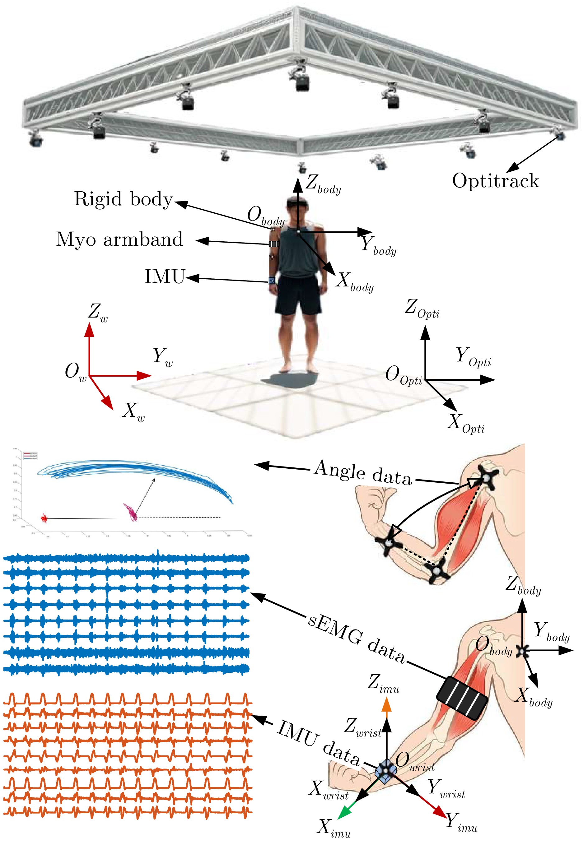
本文考虑了一类基于多通道表面肌电和惯性融合的人体运动估计问题. 如图1所示, 本文以人体上肢运动估计为例, 将八通道肌电传感器穿戴于大臂来检测上肢肌肉的状态, 同时将一个惯性传感器(由加速度计、陀螺仪和磁力计组成)固定在手腕处来估计小臂的运动状态. $ O_{w}\text{-}X_{w}Y_{w}Z_{w} $为全局坐标系({G}系), $ O_{Opti}\text{-}X_{Opti}Y_{Opti}Z_{Opti} $为光捕全局坐标系({O}系), $ O_{body}\text{-}X_{body}Y_{body}Z_{body} $为躯体坐标系({B}系), $ O_{wrist}\text{-}X_{wrist}Y_{wrist}Z_{wrist} $为手腕坐标系({W}系), $ O_{imu}\text{-}X_{imu}Y_{imu}Z_{imu} $为惯性传感器坐标系({S}系). 在运动过程中惯性传感器的坐标系会随手腕运动而变化, 而且肢体运动姿态与身体朝向密切相关, 为此, 需要建立坐标转换来描述肢体在躯体坐标系中的姿态. 为了便于坐标系转换, 简化实验, 在光捕系统进行标定时, 令光捕全局坐标系({O}系)与全局坐标系({G}系)指向相同, 即转换矩阵$ R^G_O $为单位阵. 同时, 令腕部坐标系与惯性坐标系重合, 即转换矩阵$ R^S_W $也为单位阵. 根据光捕系统中躯体的刚体坐标系可以求得{O}系与{B}系之间转换矩阵$ R^B_O $, 同时利用IMU静止时, 测到的重力加速度和磁感应强度两个矢量计算出{G}系与{S}系之间旋转矩阵$ R^G_S $, 那么, 通过惯性传感器相对于躯体的转换矩阵$ R^B_S=R^G_SR^O_GR^B_O $, 可以得到肢体在躯体坐标系中的姿态信息$ {{o}^{imu}_{k, B}}= R^B_SR^S_W $.
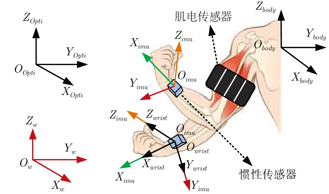 图 1 多传感器融合的人体肢体估计示意图Fig. 1 Multi-sensor fusion human body limb estimation schematic diagram
为了挖掘原始观测数据的深层次特征, 利用卷积神经网络(Convolutional neural networks, CNN)将原始观测数据$ {{o}_k} $提炼为观测特征$ {z_k} $, 并将$ {z_k} $作为观测信号建模如下:
$$ {z_k} = {g^\theta }({{o}_k}) $$ (1) 其中, $ {g^\theta }\left( \cdot \right) $为观测网络. 由于观测网络的引入以及多维观测的复杂性, 往往难以描述准确的观测模型. 在此, 利用LSTM网络去学习各量测和运动状态之间的关系, 并建立观测模型如下:
$$ z_k^{emg} = {\rm{LSTM}}_h^{emg}({x_k}) + v_k^{emg} $$ (2) $$ z_k^{imu} = {\rm{LSTM}}_h^{imu}({x_k}) + v_k^{imu} $$ (3) $ {\rm{LST}}{{\rm{M}}_h} $表示用于学习观测函数的网络模块, ${x_k} = [ {{{( {{\theta _k}} )}{}^{\rm{T}}}}\;\;{{{( {{{\dot \theta }_k}} )}{}^{\rm{T}}}} ]^{\rm{T}}$表示$ k $时刻上肢关节状态向量, $ {z_k^{emg}={g^\theta }({o^{emg}_k})} $表示$ k $时刻肌电特征向量, $ {o^{emg}_k} $为整流后的肌电幅值, $ {z_k^{imu}={g^\theta }({o^{imu}_{k, B}})} $表示$ k $时刻姿态特征向量, $ {o^{imu}_{k, B}} $为肢体相对于躯体的姿态角(roll、pitch、yaw), $ {v_k} $为$ k $时刻观测噪声. 同时, 对人体运动建模如下:
$$ {x_k} = f({x_{k - 1}, a_{k-1}}) + {w_k} $$ (4) 其中, $f( {x_{k}, a_{k}}) = \left[ {\begin{aligned} {{\theta _k} + {{\dot \theta }_k} \cdot {T_s}}\;\;\;\;\;\;\;\;\\ {{{\dot \theta }_k} + (\tfrac{{{a_k} + g\sin\theta }}{l}) \cdot {T_s}} \end{aligned}} \right]$为系统非线性状态方程, $ a_{k} $为惯性传感器测得的加速度, $ g $为重力加速度, $ l $ 为小臂长度, $ T_s $为采样时间, $ {w_k} $为$ k $时刻系统噪声, 且$ {w_k} $和$ v_k $为互不相关的零均值高斯白噪声.
虽然观测网络的引入能提取原始数据中深层次的特征, 但其依赖于训练数据, 而肌电和惯性传感器信号具有时变性[24-27], 在一定程度上增加了信息提取的难度. 为此, 设计了一种基于多通道表面肌电和惯性融合的高斯滤波网络, 利用序贯融合的方式实现互补性传感器观测融合, 同时, 采用渐进量测更新对量测特征的不确定性进行补偿.
2. 运动估计方法
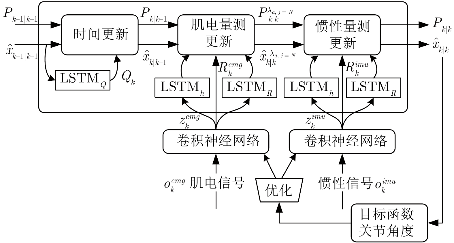
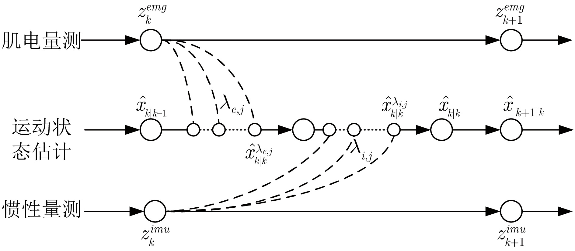
如图2所示, 利用卷积神经网络分别提取肌电和惯性信号的量测特征$ z_k^{emg} $和$ z_k^{imu} $. 同时, 设计了${\rm{LSTM}} _{Q} $和${\rm{LSTM}} _R $模块来学习噪声统计特性$ {Q_{k}} $和$ {R_{k}} $. 其次, 利用UT变换将用于学习量测函数的$ {\rm{LSTM}}_h $模块输出线性化. 考虑到肌电信号具有超前性, 通常在肢体运动之前产生[1], 因此, 采用序贯渐进量测更新方法灵活地融合肌电和惯性传感器量测特征, 以逐步更新状态估计, 从而减小线性化误差. 最后, 利用真值与估计值 $ \hat{x}_{k|k} $的偏差优化滤波网络的权重参数, 以此学习合适的状态转移过程.
2.1 序贯渐进高斯滤波网络
贝叶斯滤波是一种常见的用于递归估计未知概率密度函数的概率方法, 它包括两个阶段:
预测:
$$ \begin{split} &p(x_{k}|Z_{1:k-1})=\\ &\qquad\int p\left(x_{k}|x_{k-1}\right)p(x_{k-1}|Z_{1:k-1}){\rm d}x_{k-1} \end{split} $$ (5) 量测更新:
$$ p(x_k|Z_{1:k})=\frac{p(z_k|x_k)p(x_k|Z_{1:k-1})}{\int p(z_k|x_k)p(x_k|Z_{1:k-1}){\rm d}x_k}$$ (6) 式中, $ p(\cdot) $表示概率密度函数, $ Z_{1:k-1} $=$ \{z_{1} $, $ z_{2}, {\cdots} $, $ z_{k-1}\} $为1到$ {k-1} $ 时刻所有量测. 对于系统(4), 结合UT变换, 可以计算系统先验均值$ \hat x_{k|k-1} $和协方差$ P_{k|k-1} $为:
$$ \begin{split} &\hat x_{k|k-1} =\int x_{k}p(x_{k-1}|Z_{1:k-1}){\rm d}x_{k-1}=\\ &\qquad\int f({x}_{k-1}){\rm N}\left(x_{k};\hat{x}_{k-1|k-1}, P_{k-1|k-1}\right){\rm d}x_{k-1}\approx\\ &\qquad\sum_{i=0}^{2n}W_{i}^{m}f({\chi_{k-1|k-1}^{i}})\\[-15pt] \end{split} $$ (7) $$ \begin{split} &P_{k|k-1}=\int\left(x_{k}-\hat{x}_{k|k-1}\right)\left(x_{k}-\hat{x}_{k|k-1}\right)^{\rm{T}}\;\times\\ &\quad p(x_{k-1}|Z_{1:k-1}){\rm d}x_{k-1}=\int f({x}_{k-1})f^{\rm{T}}({x}_{k-1})\;\times \\ &\quad{\rm N}(x_k;\hat{x}_{k-1|k-1}, P_{k-1|k-1}){\rm d}x_{k-1}-\hat{x}_{k|k-1}\hat{x}_{k|k-1}^{\rm{T}}\;+\\ &\quad{Q}_{k-1}\approx\sum\limits_{i = 0}^{2n} {W_i^c} f(\chi _{k - 1|k - 1}^i){f^{\rm{T}}}(\chi _{k - 1|k - 1}^i)\;- \\&\quad{{\hat x}_{k|k - 1}}\hat x_{k|k - 1}^{\rm{T}} + {Q_{k-1}}\\[-15pt] \end{split} $$ (8) $N(\cdot) $为高斯分布, $ {W_i^m} $ 和$ {W_i^c} $, $ i=0, \; 1, \; \cdots, \; 2n $是均值和协方差计算中的权值, $ {\chi _{k-1|k-1}^{i}} $为生成的sigma点, $ {Q_k} $为系统噪声协方差. 考虑到噪声统计特性通常隐藏在时序数据中, 而LSTM能够充分捕获时序数据之间的关联性, 为此直接利用LSTM模块从系统状态向量中学习$ {Q_k} $.
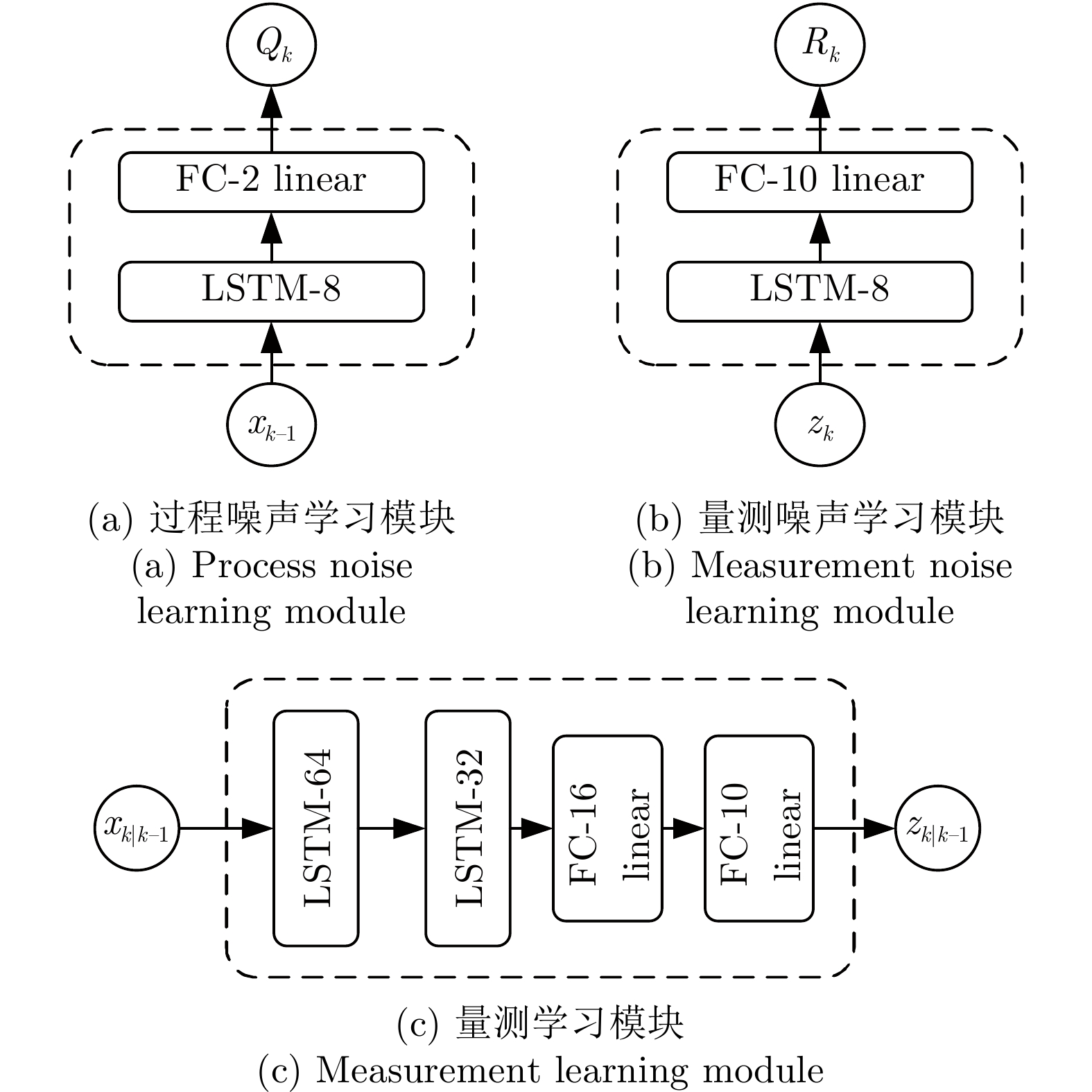
$$ {Q_k} = {\rm{LST}}{{\rm{M}}_Q}({x_{k - 1}}, c_{k - 1}^Q) $$ (9) $ {\rm{LSTM}}_Q $表示用于学习系统中$ Q_{k} $的LSTM模块, $ c_{k-1}^Q $是上一时刻$ {\rm{LSTM}}_Q $的隐藏单元. $ {\rm{LSTM}}_{Q} $结构如图3(a)所示, 由1层LSTM和1个全连接层组成, LSTM层由8个隐藏单元, 1个归一化层和1个LeakyReLU激活函数组成, 全连接层有2个隐藏单元.
如图4所示, 在序贯渐进高斯滤波网络中, 量测更新由几个子过程组成, 在每个子过程中, 采集到的传感器测量将依次用于更新状态估计.
注1. 在卡尔曼滤波中, 当量测测量向量的维数很大时, 求解增益阵$ K $时求逆的阶数将很高(通常, 求逆的计算量与矩阵阶数的三次方近似成正比). 特别地, 在高维矩阵运算时, 可能会出现发生数值溢出近似、奇异矩阵等问题, 从而导致估计系统不稳定. 而在序贯渐进高斯滤波中, 将传感器测量分解为多个分量, 使得对高阶矩阵的求逆转变为对低阶矩阵求逆, 同时利用传感器的互补优势逐一渐进地引入信息, 来降低线性化误差以及提高滤波的稳定性. 这就改善了高维量测引发的模型融合估计效率降低以及系统不稳定等问题.
在渐进高斯滤波中[28-29], 通过引入伪时间长度$ {\lambda_j}={\lambda_{j-1}}+{\Delta_j} $ ($ {\Delta_j} $为渐进步长, $ {\lambda_{0}}=0) $, 对观测中的不确定性进行补偿. 其中, 似然函数可以写成如下形式:
$$ \begin{split} p(z_k|x_k)=\;&\frac{1}{\sqrt{2\pi\left|R_k\right|}}\exp\{-\frac{1}{2}[z_k-h(x_k)]^{{\rm{T}}}\;\times \\ &\big(R_{k}\big)^{-1}\big[z_{k}-h(x_{k})\big]\}\;= \\ &C_{N}\prod_{j=1}^{N}\frac{1}{\sqrt{\left|\frac{2\pi R_k}{\Delta_{j}}\right|}}\exp\{-\frac{1}{2}[z_k-h(x_k)]^{{\rm{T}}}\;\times \\ &\left(\frac{R_{k}}{\Delta_{j}}\right)^{-1}\left[\left.z_{k}-h\left(x_{k}\right)\right]\right\}\;= \\ &C_{N}\prod_{j=1}^{N}p(z_k, \Delta_{j}|x_k)\\[-15pt] \end{split} $$ (10) $ {p ({z_k}, {\Delta _j}|{x_k})} $为渐进似然函数. $ {C_N} $为归一化常量, $ C_N=\left(1/\sqrt{2\pi R_k}\right)^{N-1}\prod_{j=1}^N\sqrt{\Delta_j} $, $ {\Delta _j}=\frac{1}{N} $为渐进步长. $ {N} $为渐进步数, 理论上, 较大的$ {N} $可以提供更精确的状态估计, 较小的$ {N} $能降低计算复杂度, 但可能无法充分捕捉系统的非线性行为, 导致滤波估计不准确. 在实际应用中, 通常需要进行实验和调整, 以找到最佳的$ N $值. 在本文中, 经过权衡, $ {N} $的取值为20. 根据贝叶斯准则, 伪时间$ {\lambda_{j+1}} $对应的渐进后验概率密度函数为:
$$ \begin{split} p( {x_k}|&{\lambda _{j + 1}}, {z_k}, {Z_{1:k - 1}})=\\ &p({x_k}|{\lambda _j} + {\Delta _j}, {z_k}, {Z_{1:k - 1}})=\\ &\frac{{p({z_k}, {\Delta _j}|{x_k})p({x_k}|{\lambda _j}, {Z_{1:k - 1}})}}{{\int {p({z_k}, {\Delta _j}|{x_k})p({x_k}, {\lambda _j}|{Z_{1:k - 1}}){\rm d}{x_k}} }} \end{split} $$ (11) 对于系统(2), 假设$ {p(z_k^{emg}, \Delta_j|x_k)} $服从零均值协方差为$ {R_k^{emg}/\Delta_j} $的高斯分布, 即
$$ \begin{split} &p(z_k^{emg}, {\Delta _j}|{x_k})= \\ &\qquad\frac{1}{{\sqrt {\left| {\frac{{2\pi R_k^{emg}}}{{{\Delta _j}}}} \right|} }}\exp \Bigg\{ { - \frac{1}{2}}{\left[ {z_k^{emg} - {\rm{LSTM}}_{{h}}^{{{emg}}}\left( {{x_k}} \right)} \right]^{\rm{T}}}\;\times \\ &\qquad {{{\left( {\frac{{R_k^{emg}}}{{{\Delta _j}}}} \right)}^{ - 1}}\left[ {z_k^{emg} - {\rm{LSTM}}_{{h}}^{{{emg}}}\left( {{x_k}} \right)} \right]} \Bigg\}\\[-20pt] \end{split} $$ (12) $ {\rm{LSTM}}^{emg}_{h} $为学习的肌电观测函数, $ {R^{emg}_k} $由LSTM模块直接从系统状态向量中学习得到, 结构分别如图3(b)、3(c)所示. 其中, $ {\rm{LSTM}}^{emg}_{h} $由2个LSTM层和2个全连接层组成, 每层LSTM由1个归一化层和1个LeakyReLU激活函数组成. 第1层LSTM中有64个隐藏单元, 第2层LSTM中有32个隐藏单元. 第1个全连接层有16个隐藏单元, 第2个全连接层有10个隐藏单元. $ {\rm{LSTM}}_{R} $ 由1层LSTM和1个全连接层组成, LSTM层由8个隐藏单元、1个归一化层和1个LeakyReLU激活函数组成, 全连接层有10个隐藏单元.
假设渐进联合概率密度函数为高斯分布:
$$ \begin{split} &p({x_k}, z_k^{emg}, {\lambda _{e, j + 1}}|{Z_{1:k - 1}}) = {\rm N} \Biggr( {\left[ {\begin{array}{*{20}{l}} {{x_k}}\\ {{z_k}} \end{array}} \right];} \\ &\qquad {\left[ {\begin{array}{*{20}{l}} {\hat x_{k|k}^{{\lambda _{e, j}}}}\\ {\hat z_{k|k}^{emg, {\lambda _{e, j + 1}}}} \end{array}} \right], \left[ {\begin{array}{*{20}{l}} {P_{xx, k|k}^{{\lambda _{e, j}}}}&{P_{xz, k|k}^{{\lambda _{e, j + 1}}}}\\ {P_{zx, k|k}^{{\lambda _{e, j + 1}}}}&{P_{zz, k|k }^{{\lambda _{e, j + 1}}}} \end{array}} \right]} \Biggr) \end{split} $$ (13) 则渐进后验概率密度函数为:
$$ \begin{split} p( & x_{k}|\lambda_{{e}, j+1}, z_{k}^{emg}, Z_{1:k-1})=\\ &\qquad{\rm N}\left(x_k; \hat{x}_{k|k}^{\lambda_{e, j+1}}, P_{k|k}^{\lambda_{e, j+1}}\right) \end{split} $$ (14) 结合UT变换计算量测预测值及其协方差:
$$ \begin{split} &\hat z_{k|k}^{{{emg}, \lambda _{e, j}}} =\\ &\quad\int\int{{z_{k}^{emg}}p({x_k}, z_k^e, {\lambda _{e, j }}|{Z_{1:k - 1}}){\rm d}{z_k}{\rm d}{x_k}}\;=\\ &\quad\int {\left\{ {\int {{z_{k}^{emg}}p(z_k^{emg}, {\Delta _j}|{x_k}){\rm d}{z_k}} } \right\}}\; \times \\ &\quad p(x_{k}|\lambda_{e, j-1}, z_{k}^{emg}, Z_{1:k-1}){\rm d}{x_k}\;\approx \\ &\quad\int {{\rm{LSTM}}^{emg}_{h}({x_k})}{\rm N}\left(x_k; \hat{x}_{k|k}^{\lambda_{e, j-1}}, P_{k|k}^{\lambda_{e, j-1}}\right){\rm d}{x_k}\;\approx \\ &\quad\sum\limits_{i = 0}^{2n} W_i^m{{\rm{LSTM}}^{emg}_{h}}(\chi _{i, k|k}^{{\lambda _{e, j - 1}}}) \\[-15pt]\end{split} $$ (15) $$ \begin{split} &P_{zz, k|k}^{{\lambda _{e, j}}} = \\ &\;\;\int {\int {(z_k^{emg} - \hat z_{k|k}^{emg, {\lambda _{e, j}}})} } {(z_k^{emg} - \hat z_{k|k}^{emg, {\lambda _{e, j}}})^{\rm{T}}} \;\times \\ &\;\;p({x_k}, z_k^{emg}, {\lambda _{e, j}}|{Z_{1:k - 1}}){\rm{d}}{z_k}{\rm{d}}{x_k} \;= \\ &\;\;\int {\left( {\int {z_k^{emg}} {{(z_k^{emg})}^{\rm{T}}}p(z_k^{emg}, {\Delta _j}|{x_k}){\rm{d}}{z_k}} \right)}\; \times \\ &\;\;p({x_k}, {\lambda _{e, j - 1}}|{Z_{1:k - 1}}){\rm{d}}{x_k} - \hat z_{k\mid k}^{emg, {\lambda _{e, j}}}{\left( {\hat z_{k\mid k}^{emg, {\lambda _{e, j}}}} \right)^{\rm{T}}} \approx \\ &\;\;\frac{{R_k^{emg}}}{{{\Delta _j}}} - \hat z_{k\mid k}^{emg, {\lambda _{e, j}}}{(\hat z_{k\mid k}^{emg, {\lambda _{e, j}}})^{\rm{T}}} + \int {{\rm{LSTM}}_h^{emg}\left( {{x_k}} \right)} \; \times \\ &\;\;{\left[ {{\rm{LSTM}}_h^{emg}\left( {{x_k}} \right)} \right]^{\rm{T}}}{\rm N}\left( {{x_k};\hat x_{k|k}^{{\lambda _{e, j - 1}}}, P_{k|k}^{{\lambda _{e, j - 1}}}} \right){\rm{d}}{x_k} \;= \\ &\;\;\sum\limits_{i = 0}^{2n}{W_i^c}{\rm{LSTM}}_h^{emg} \left( {\chi _{i, k|k}^{{\lambda _{e, j - 1}}}} \right) {\left[ {{\rm{LSTM}}_h^{emg} \left( {\chi _{i, k|k}^{{\lambda _{e, j - 1}}}} \right)} \right]^{\rm{T}}}+\\ &\;\;\frac{{R_k^{emg}}}{{{\Delta _j}}} - \hat z_{k|k}^{emg, {\lambda _{e, j}}}{\left( {\hat z_{k|k}^{emg, {\lambda _{e, j}}}} \right)^{\rm{T}}} \\[-15pt]\end{split} $$ (16) 计算先验状态估计值与观测预测值间的互协方差:
$$ \begin{split} &P_{xz, k|k}^{{\lambda _{e, j}}} = \int {\int {\left( {{x_k} - \hat x_{k|k}^{{\lambda _{e, j - 1}}}} \right)} } {\left( {z_k^{emg} - \hat z_{k|k}^{{emg}, {\lambda _{e, j}}}} \right)^{\rm{T}}}\;\times\\ &\qquad p({x_k}, z_k^{emg}, {\lambda _{e, j }}|{Z_{1:k - 1}}){\rm d}{z_k}{\rm d}{x_k}\;-\\ &\qquad \hat x_{k|k}^{{\lambda _{e, j - 1}}}{\left( {\hat z_{k|k}^{{emg}, {\lambda _{e, j}}}} \right)^{\rm{T}}}\approx\int {{x_k}{{\left[ {{\rm{LSTM}}_{{h}}^{{{emg}}}\left( {{x_k}} \right)} \right]}^{\rm{T}}}}\;\times\\ &\qquad {\rm N}\left( {{x_k};\hat x_{k|k}^{{\lambda _{e, j - 1}}}, P_{k|k}^{{\lambda _{e, j - 1}}}} \right){\rm d}{x_k}\; - \\ &\qquad \hat x_{k\mid k}^{{emg}, {\lambda _{e, j - 1}}}{(\hat z_{k\mid k}^{{emg}, {\lambda _{e, j}}})^{\rm{T}}}\;\approx \\ &\qquad \sum\limits_{i = 0}^{2n} {W_i^c} \chi _{i, k|k}^{{\lambda _{e, j - 1}}}{\left[ {{\rm{LSTM}}_{{h}}^{{{emg}}}\left( {\chi _{i, k|k}^{{\lambda _{e, j - 1}}}} \right)}\right]^{\rm{T}}}\; -\\ &\qquad \hat x_{k\mid k}^{{emg}, {\lambda _{e, j - 1}}}{(\hat z_{k\mid k}^{{emg}, {\lambda _{e, j}}})^{\rm{T}}}\\[-15pt] \end{split} $$ (17) 其中, $ \chi_{i, k|k}^{{\lambda_{e, j}}} $和$ {W_i^c} $为对应的sigma点与权值. 由式(15) ~ (17)可得状态估计和估计方差为:
$$ \hat x_{k|k}^{{\lambda _{e, j}}} = \hat x_{k|k}^{{\lambda _{e, j - 1}}} + K_{k|k}^{{\lambda _{e, j}}}({z_{k}^{emg}} - \hat z_{k|k}^{{{emg}, \lambda _{e, j}}}) $$ (18) $$ P_{k|k}^{{\lambda _{e, j}}} = P_{k|k}^{{\lambda _{e, j - 1}}} - K_{k|k}^{{\lambda _{e, j}}}P_{zz, k|k}^{{\lambda _{e, j}}}{(K_{k|k}^{{\lambda _{e, j}}})^{\rm{T}}} $$ (19) 其中, 渐进卡尔曼增益为:
$$ K_{k|k}^{{\lambda _{e, j}}} = P_{xz, k|k}^{{\lambda _{e, j}}}{(P_{zz, k|k}^{{\lambda _{e, j}}})^{ - 1}} $$ (20) 伪时间$ {\lambda _{e, j}} $从0走向1的过程也即从先验走向后验的过程, 对应的观测噪声协方差间接趋向 $ {R^{emg}_k} $. 从而将观测不确定性补偿问题转换为了伪时间长度的控制问题.
同理, 融合惯性量测$ {z_k^{imu}} $, 更新状态估计值和协方差:
$$ \hat x_{k|k}^{{\lambda _{i, j}}} = \hat x_{k|k}^{{\lambda _{i, j - 1}}} + K_{k|k}^{{\lambda _{i, j}}}({z_{k}^{imu}} - \hat z_{k|k}^{{{imu}, \lambda _{i, j}}}) $$ (21) $$ P_{k|k}^{{\lambda _{i, j}}} = P_{k|k}^{{\lambda _{i, j - 1}}} - K_{k|k}^{{\lambda _{i, j}}}P_{zz, k|k}^{{\lambda _{i, j}}}{(K_{k|k}^{{\lambda _{i, j}}})^{\rm{T}}} $$ (22) 且满足:
$$ \left\{ {\begin{aligned} &{\hat x_{k|k}^{{\lambda _{i, j = 0}}} = \hat x_{k|k}^{{\lambda _{e, j=N}}}}\\ &{ P_{k|k}^{{\lambda _{i, j = 0}}} = P_{k|k}^{{\lambda _{e, j=N}}}} \end{aligned}} \right. $$ (23) 其中, 渐进卡尔曼增益矩阵为:
$$ K_{k|k}^{{\lambda _{i, j}}} = P_{xz, k|k}^{{\lambda _{i, j}}}{( P_{zz, k|k}^{{\lambda _{i, j}}})^{ - 1}} $$ (24) 状态和观测互协方差, 预测观测协方差分别为:
$$ \begin{split} P_{xz, k|k}^{{\lambda _{i, j}}} \approx \;&\sum\limits_{l = 0}^{2n} {W_l^c} \left[ {\chi _{l, k|k}^{{\lambda _{i, j-1}}} - x_{k|k}^{{\lambda _{i, j - 1}}}} \right]\;\times\\ &{\left[ {{{{\rm{LSTM}}^{{{imu}}}_{h}}}(\chi _{l, k|k}^{{\lambda _{i, j-1}}}) - \hat z_{k|k}^{{imu}, {\lambda _{i, j}}}} \right]^{\rm{T}}} \end{split} $$ (25) $$ \begin{split} &P_{zz, k|k}^{{\lambda _{i, j}}}\approx\sum\limits_{l = 0}^{2n} {W_l^c} \left[ {{{\rm{LSTM}}^{{{imu}}}_{h}}(\chi _{l, k|k}^{{\lambda _{i, j-1}}}) - \hat z_{k|k}^{{{{imu}}}, {\lambda _{i, j}}}} \right]\;\times\\ &\qquad{\left[ {{{{\rm{LSTM}}^{{{imu}}}_{h}}}(\chi _{l, k|k}^{{\lambda _{i, j-1}}}) - \hat z_{k|k}^{{imu}, {\lambda _{i, j}}}} \right]^{\rm{T}}} + \frac{{R_k^{imu}}}{\Delta_j } \end{split} $$ (26) 为了保证各观测模块和噪声统计模块学习到合理的映射, 将真值与估计值的偏差作为序贯高斯滤波网络的损失:
$$ \begin{split} L\left( \theta \right) =\;& \frac{1}{T}\sum\limits_{k = 1}^T {\left( {{{\left\| {{x_k} - \hat x_{k|k - 1}^{}} \right\|}^2} \;+ } \right.} \\ &\left. {{{\left\| {{x_k} - \hat x_{k|k}^{{\lambda _{e, j = N}}}} \right\|}^2} + {{\left\| {{x_k} - \hat x_{k|k}^{{\lambda _{i, j = N}}}} \right\|}^2}} \right) \end{split} $$ (27) 其中, $ T $表示单个训练样本的时间步长, $ {x_k} $表示真值, $ {\hat x}_{k|k - 1} $表示状态预测值, $ \hat x_{k|k}^{{\lambda _{e, j=N}}} $和$ \hat x_{k|k}^{{\lambda _{i, j=N}}} $分别为$ {N} $步时肌电和惯性信号的观测更新值.
算法 1. 深度序贯渐进高斯滤波算法
1: 初始化;
2: while
3: 利用卷积网络提取观测特征;
4: 利用式(7) ~ (9)进行时间更新;
5: for $ j = 1:N $ do
6: 利用式(10) ~ (20)融合肌电观测;
7: end for
8: for $ j = 1:N $ do
9: 利用式(21) ~ (26)融合惯性观测;
10: end for
11: end while
3. 实验
为了验证该融合算法的可行性, 本文以人体上肢肘关节为例, 对$12 $名健康受试者的左右手肘关节进行了实验, 其中男性8名, 女性4名, 平均年龄为25.3 ± 4.8岁; 平均身高为165.3 ± 13.6厘米; 平均体重为68.5 ± 10.2千克. 实验前, 获得了每位受试者的书面同意.
3.1 数据采集
如图5所示, 实验采用Myo臂环作为表面肌电信号的采集系统, 其信号采样频率为100 Hz, 能采集8通道数据. 同时利用1个9轴IMU对受试者小臂的惯性信号进行采集, 采样频率100 Hz. 对于关节角度采集部分, 采用Optitrack视觉捕捉系统获取上肢关节运动特性, 分别用4个刚体描述腕部、肘部、肩部和躯体坐标, 采样频率100 Hz. 在数据采集过程中, 受试者站在Optitrack工作区间, 手臂自然下垂, 进行屈肘运动, 弯曲至最大角度位置. 在短暂停顿后进行伸展, 最后恢复到初始位置. 每次实验进行15组肘关节屈伸运动. 每个测试者进行5组重复实验, 为了防止肌肉疲劳, 每组实验之间设置5分钟的休息时间, 实验持续约35分钟.
3.2 特征提取
本文采用CNN提取原始数据的深层特征. 具体而言, 采用滑动窗口法分别获得大小为$ {{L}}\times{{C_1}} $的表面肌电信号矩阵和大小为$ {{L}}\times{C_2} $的惯性信息矩阵. 其中, $ {{L}} $表示窗口长度, $ {{C_1}} $和$ {C_2} $ 分别表示肌电传感器和惯性传感器通道数. 本文的CNN由4个卷积块和2个全连接块组成. 每个卷积块由1个卷积层、1个批归一化层、1个ReLU激活函数层、1个最大池化层和1个丢弃层组成. 卷积层内核大小为3, 步幅为1. 第1和第2个卷积块有16个核, 而第3和第4卷积块有32个核. 每个全连接块都由批归一化层、ReLU激活函数层和丢失层组成. 第1个全连接块有100个隐藏单元, 第2个全连接块有10个隐藏单元. 第2个全连接块的输出将被用作观测特征.
3.3 模型参数设置
实验中的所有网络模型都基于Python语言实现, 由Pytorch1.10库搭建, 在英特尔i7*10750H处理器以及英伟达RTX 2070显卡上完成训练和测试. 网络模型训练总轮次设置为60, 训练的批次设置为32, 选用Adam作为实验训练的优化器, CNN特征提取模块训练阶段初始学习率为0.001, 且学习率每隔10轮降为原来的一半, 所有LSTM模块均使用初始化权重, 初始学习率为0.001, 每隔5轮对学习率进行一次调整, 衰减率为0.8. 数据集前60%用于训练, 剩余40%用于测试. 为确保实验的可靠性, 在对比模型上都设置相同的超参数.
4. 实验结果与分析
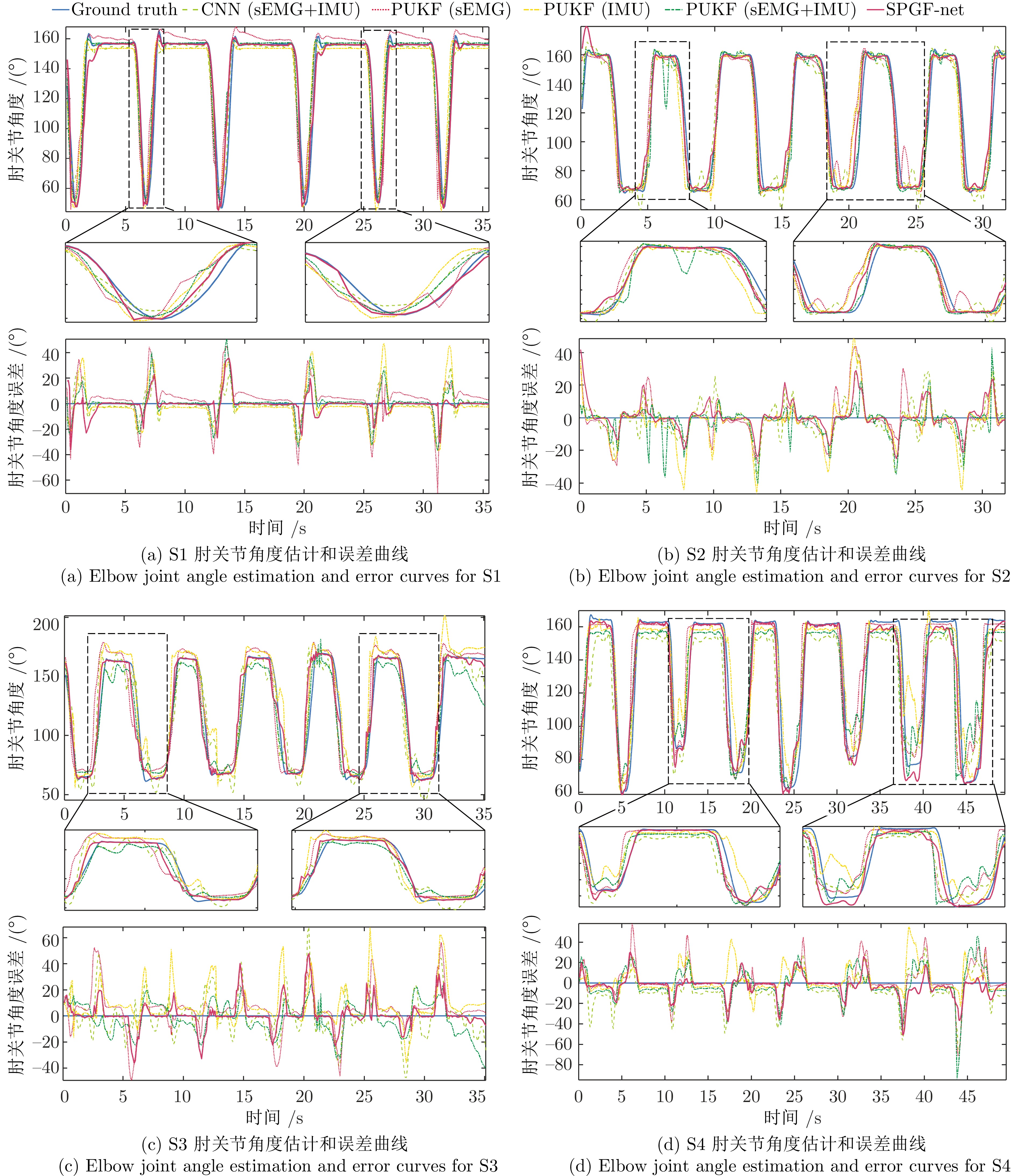
本文将相关系数(R2)和均方根误差(RMSE)作为性能指标对融合模型进行评估, 并统计了各网络模型的浮点运算数 (FLOPs)和参数数量(Params). 其中, R2表明估计的曲线与测量的关节运动的相关程度, 而RMSE计算估计值与测量值之间的幅值差异. 本文选择卷积神经网络(sEMG和IMU信号为输入, 对高维特征进行拼接) 和渐进无迹卡尔曼滤波网络(分别以sEMG和IMU信号为输入, 对提取的特征向量进行建模; 将sEMG和IMU信号作为输入, 对特征融合后的特征向量进行建模)作为模型比较的基线方法. 以S1 ~ S4四名测试者右手的估计结果为例, 图6展示了四名受试者在五种模型下的肘关节角度估计和误差曲线. 五种方法都可以从表面肌电信号中有效地重建肘关节运动.
由于传感器布局、个数等因素, 基于sEMG的人体运动估计结果总体上略高于基于IMU的人体运动估计结果. PUKF-net通过利用先验知识和渐进量测对卷积神经网络提取的特征向量进行校正和不确定性补偿取得了相对光滑的估计曲线, 但由于单一信号有效信息有限, PUKF (sEMG)和PUKF(IMU)的估计结果在整体上还是低于CNN (sEMG+IMU). PUKF (sEMG+IMU)在CNN特征融合的基础上利用卡尔曼滤波框架提高了网络的估计性能和稳定性, SPGF-net在PUKF的基础上通过序贯融合肌电和惯性量测特征向量, 发挥了肌电和惯性信号的互补优势, 得到了相对光滑的曲线. 如图6(b)所示, 在18 s至26 s, CNN (sEMG+IMU)、PUKF (sEMG)和PUKF (IMU)估计测试者2的关节角度曲线都出现了不同程度的波动, 而SPGF-net的估计曲线(紫色实线)相对光滑且整体上更接近Optitrack真实值(蓝色实线). 为了定量比较几种方法的估计性能, 表1总结了CNN (sEMG+IMU)、PUKF (sEMG)、PUKF (IMU)、PUKF (sEMG+IMU)和SPGF-net五种方法的平均性能(平均值 ± 标准差). 其中, R2分别为0.854 ± 0.093、0.847 ± 0.080、0.838 ± 0.080、0.865 ± 0.080、0.884 ± 0.060, RMSE分别为14.52 ± 4.21、15.07 ± 3.54、15.64 ± 3.46、13.99 ± 3.96、12.99 ± 3.51. 与其他四种方法相比, SPGF-net通过序贯融合的方式提高了模型的精度和稳定性. 相较于PUKF (sEMG)模型而言, 在肘关节角度估计中的RMSE平均下降了13.8%, 相关系数平均提高了4.36%.
表 1 五种模型性能评价Table 1 The performance evaluation of five models测试者 均方根误差 (RMSE) 相关系数(R2) CNN
(sEMG+IMU)PUKF
(sEMG)PUKF
(IMU)PUKF
(sEMG+IMU)SPGF-net CNN
(sEMG+IMU)PUKF
(sEMG)PUKF
(IMU)PUKF
(sEMG+IMU)SPGF-net S1 9.75 11.91 12.48 9.56 9.27 0.922 0.884 0.872 0.925 0.930 S2 11.65 12.18 13.25 10.89 9.78 0.917 0.913 0.893 0.923 0.941 S3 16.18 15.90 16.42 15.63 14.15 0.864 0.868 0.859 0.876 0.896 S4 15.66 16.18 16.95 14.57 13.45 0.825 0.822 0.816 0.832 0.847 S5 24.24 23.30 23.79 22.74 18.98 0.594 0.624 0.609 0.651 0.751 S6 10.15 11.43 11.65 9.96 8.91 0.937 0.920 0.917 0.941 0.949 S7 16.31 16.62 17.19 16.13 15.90 0.856 0.851 0.847 0.860 0.869 S8 16.84 16.37 16.53 16.30 16.23 0.807 0.809 0.805 0.813 0.821 S9 9.23 9.95 10.86 8.82 7.73 0.930 0.918 0.903 0.938 0.951 S10 14.97 15.74 16.17 14.53 14.00 0.849 0.831 0.821 0.853 0.866 S11 16.86 17.19 17.66 16.62 15.78 0.852 0.846 0.838 0.857 0.864 S12 12.46 14.09 14.83 12.13 11.74 0.905 0.885 0.870 0.909 0.924 均值 14.52 15.07 15.64 13.99 12.99 0.854 0.847 0.838 0.865 0.884 标准差 4.21 3.54 3.46 3.96 3.51 0.093 0.080 0.080 0.080 0.060 为了评估各网络模型的复杂度, 本文统计了各网络模型浮点运算数(FLOPs)和网络模型参数数量(Params), 如表2所示. 由于观测网络模型的增加, 整个网络模型的计算量和参数总量也有一定程度的增加, 相较于提升的性能而言, 模型复杂度的增加在接受范围之内.
表 2 五种模型的复杂度Table 2 The complexity of five modelsCNN (sEMG+
IMU)PUKF (sEMG) PUKF (IMU) PUKF (sEMG+
IMU)SPGF-net FLOPs 1 237 714 719 448 619 828 1 328 864 1 419 176 Params 442 337 256 511 255 971 473 970 505 614 5. 结束语
本文设计了一种面向多通道表面肌电和惯性融合的序贯渐进高斯滤波网络, 实现了人体上肢运动估计. 利用卷积神经网络提取观测特征向量, 与常见的特征拼接不同, SPGF-net采用序贯融合的方式, 融合异构传感器量测. 特别地, 通过渐进量测更新的方法, 对观测网络的不确定性进行补偿. 实验结果表明所提出的融合方法可有效提高人体上肢关节角度估计的精度和稳定性. 本文仅对单个肘关节运动进行了估计, 然而多关节协同对模型要求更高. 在未来工作中, 将考虑多关节的协同和更复杂场景下的运动估计, 来评估我们的模型, 并进一步提高高斯滤波网络的自适应性, 同时将充分发挥深度学习在自适应滤波中的优势, 研究更为智能且泛用的自适应滤波策略.
-
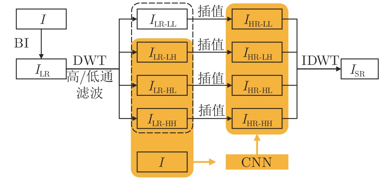
图 6 基于传统小波变换和与深度学习相结合的小波变换SR重建方法流程图
Fig. 6 SR reconstruction method based on traditional wavelet transform and wavelet transform combined with deep learning
表 1 典型深度学习网络内部结构
Table 1 The internal structure of a typical deep learning network
方法 网络结构 作用 VDSR[78] 残差学习 加快深度网络收敛 DRCN[79] 递归监督、跳跃连接 减缓梯度爆炸或梯度消失, 存储输入信号用于目标预测 DRRN[82] 全局残差学习 学习复杂特征, 帮助梯度传播 局部残差学习 携带丰富的细节信息 递归块 权值共享, 多路径递归连接 SRDenseNet[83] 密集跳跃连接 增强不同层间的特征融合 EDSR[91] 残差块 增强初始层级与深度层级的联系 MemNet[85] 内存块 自适应地学习不同内存的不同权重 递归单元 控制应该保留多少长期内存 门单元 存储多少短期内存 RDN[86] 残差密集块 读取前一个RDN状态, 增强层间连接 连续记忆机制 全局特征融合, 挖掘分层信息 SRFBN[96] 反馈块、反馈机制 共享权重, 帮助更好的高级信息表达; 高级信息回传给低级信息 RCAN[99] 通道注意力机制 分级标定图像低级和高级语义信息  下载: 导出CSV
表 2 SR网络输入及层数对照表
Table 2 Comparison of SR network input and layer number
方法 网络输入 网络层数 SRCNN LR + BI 3 FSRCNN LR 8 ESPCN LR 3 VDSR LR + BI 20 DRCN LR + BI 20 LapSRN LR 27 RED LR 30 DRRN LR + BI 52 SRDenseNet LR 64 SRGAN LR + BI 54 MemNet LR + BI 80 RDN LR 20 (RDB)
下载: 导出CSV
表 3 SR重建图像常用质量评价方法
Table 3 Common quality evaluation methods for SR reconstructed images
特点 类别 常用评估方法 适用场景 优缺点 使用方法 主观 全参考 基于评分 MOS/DMOS 不受距离、设备、光照、及观测者的视觉能力、情绪等因素影响的情况 优点: 能够真实的反映图像的直观质量, 评价结果可靠, 无技术障碍. 缺点: 无法应用数学模型对其进行描述, 耗时多、费用高. 易受观测动机、观测环境等诸多因素的影响. 根据评分表分别对参考图像和待测图像评分 客观 全参考
(真值图像 + 失真图像)基于像素 MSR/PSNR — 优点: 计算形式上非常简单, 物理意义理解也很清晰. 缺点: 未考虑将人类视觉系统特性, 单纯从数学角度来分析差异, 未与图像的感知质量产生联系. — 基于人类视觉系统 (结构和特征) SSIM/MS-SSIM/
FSIM/VIF/IFC参考图像完整的情况 优点: 从整体上直接模拟HVS(人类视觉系统)抽取对象结构的人类视觉功能, 更符合视觉感知. 缺点: 从图像像素值的全局统计出发, 未考虑人眼的局部视觉因素, 对于图像局部质量无从把握. 所有像素点对应比较 基于深度学习 NAR-DCNN[145]/
LPIPS[146]— — — — 盲参考
(失真图像)基于感知/概率模型 PI[147]/Ma[148]/
NIQE[149]/
BLIINDS[150]/
BIQI[151]/
BRISQUE[151]无参考图像的情况. 无需参考图像, 灵活性强. 优点: 直接从原始图像像素学习判别图像特征, 而不使用手工提取特征. 共性: 首先对理想图像的特征做出某种假设, 转化成一个分类或回归问题; 再为该假设建立相应的数学分析模型, 学习特征; 最后通过计算待评图像在该模型下的表现特征, 从而得到图像的质量评价结果. 特征由自然场景统计提取 基于深度学习
(网络模型)DB-CNN[152]/
RankIQA[153]/
DIQI[154]CNN/CNN+回归模型提取特征
下载: 导出CSV
-
[1] Park S C, Park M K, Kang M G. Super-resolution image reconstruction: A technical overview. IEEE Signal Processing Magazine, 2003, 20(3): 21-36. doi: 10.1109/MSP.2003.1203207 [2] Morin R, Basarab A, Kouame D. Alternating direction method of multipliers framework for super-resolution in ultrasound imaging. In: Proceedings of the 9th IEEE International Symposium on Biomedical Imaging. Barcelona, Spain: IEEE, 2012. 1595−1598 [3] Cui J, Wang Y, Huang J, Tan T, Sun Z. An iris image synthesis method based on PCA and super-resolution. In: Proceedings of the 17th International Conference on Pattern Recognition. Cambridge, UK: 2004. 471−474 [4] Nguyen K, Sridharan S, Denman S, Fookes C. Feature domain super-resolution framework for Gabor-based face and iris recognition. In: Proceedings of the 25th IEEE Conference on Computer Vision and Pattern Recognition. Providence, USA: IEEE, 2012. 2642−2649 [5] Harris J L. Diffraction and resolving power. Journal of the Optical Society of America, 1964, 54(7): 931-933. doi: 10.1364/JOSA.54.000931 [6] Goodman J W. Introduction to Fourier Optics. New York: McGraw-Hill, 1968. [7] Tsai R, Huang T. Multiframe image restoration and registration. Computer Vision and Image Processing, 1984, 1(2): 317-339. [8] Yang J, Wright J, Huang T S, Ma Y. Image super-resolution as sparse representation of raw image patches. In: Proceedings of the 26th IEEE Computer Society Conference on Computer Vision and Pattern Recognition. Anchorage, USA: IEEE, 2008. [9] Yang J, Wright J, Huang T S, Ma Y. Image super-resolution via sparse representation. IEEE Transactions on Image Processing, 2010, 19(11): 2861-2873. doi: 10.1109/TIP.2010.2050625 [10] Nguyan N, Golub G, Milanfar P. Preconditioners for regularized image super resolution. In: Proceedings of the 1999 IEEE International Conference on Acoustics, Speech, and Signal Processing. Piscataway, USA: IEEE, 1999. 3249−3252 [11] Yu G, Sapiro G, Mallat S. Solving inverse problems with piecewise linear estimators: From gaussian mixture models to structured sparsity. IEEE Transactions on Image Processing, 2012, 21(5): 2481-2499. doi: 10.1109/TIP.2011.2176743 [12] Elad M, Feuer A. Restoration of a single super resolution image from several blurred, noisy, and under sampled measured images. IEEE Transactions on Image Processing, 1997, 6(12): 1646-1658. doi: 10.1109/83.650118 [13] Timofte R, De Smet V, Van Gool L. A+: Adjusted anchored neighborhood regression for fast super-resolution. In: Proceedings of the 12th Asian Conference on Computer Vision. Singapore: 2014. 111−126 [14] Cui Z, Chang H, Shan S, Zhong B, Chen X. Deep network cascade for image super-resolution. In: Proceedings of the 13th European Conference on Computer Vision. Zurich, Switzerland: 2014. 49−64 [15] Song H, Zhang L, Wang P, Zhang K, Li X. AN adaptive L1-L2 hybrid error model to super-resolution. In: Proceedings of the 2010 IEEE International Conference on Image Processing. Hong Kong, China: IEEE, 2010. 2821−2824 [16] Wang S, Zhang L, Liang Y, Pan Q. Semi-coupled dictionary learning with applications to image super-resolution and photo-sketch synthesis. In: Proceedings of the 2012 IEEE Conference on Computer Vision and Pattern Recognition. Providence, USA: IEEE, 2012. 2216−2223 [17] Dong C, Loy C C, He K, Tang X. Image super-resolution using deep convolutional networks. IEEE Transactions on Pattern Analysis and Machine Intelligence, 2015, 38(2): 295-307. [18] Zhu Y, Zhang Y, Yuille A L. Single image super-resolution using deformable patches. In: Proceedings of the 27th IEEE Conference on Computer Vision and Pattern Recognition. Columbus, USA: IEEE, 2014. 2917−2924 [19] Gao X, Zhang K, Tao D, Li X. Image super-resolution with sparse neighbor embedding. IEEE Transactions on Image Processing, 2012, 21(7): 3194-3205. doi: 10.1109/TIP.2012.2190080 [20] Dong W, Zhang L, Shi G, Wu X. Image deblurring and super-resolution by adaptive sparse domain selection and adaptive regularization. IEEE Transactions on Image Processing, 2011, 20(7): 1838-1857. doi: 10.1109/TIP.2011.2108306 [21] 岳波. 基于学习的图像超分辨率重建方法研究[博士论文], 西安电子科技大学, 中国, 2019Yue Bo. Study on Learning-Based Image Super-Resolution Method [Ph.D. dissertation], Xidian University, China, 2019 [22] 苏衡, 周杰, 张志浩. 超分辨率图像重建方法综述[J]. 自动化学报, 2013, 39(8): 1202-1213.Su Heng, Zhou Jie, Zhang Zhi-Hao. Survey of Super-resolution Image Reconstruction Methods. Acta Automatica Sinica, 2013, 39(8): 1202-1213(in Chinese) [23] 孙旭, 李晓光, 李嘉锋, 卓力. 基于深度学习的图像超分辨率复原研究进展[J]. 自动化学报, 2017, 43(5): 697-709.Sun Xu, Li Xiao-Guang, Li Jia-Feng, Zhuo Li. Review on Deep Learning Based Image Super-resolution Restoration Algorithms. Acta Automatica Sinica, 2017, 43(5): 697-709(in Chinese) [24] Wang Z H, Chen J, C. H. Hoi S. Deep Learning for Image Super-resolution: A Survey. IEEE Transactions on Pattern Analysis and Machine Intelligence2021, 43(10): 3365-3387 [25] Baker S, Kanade T. Limits on super-resolution and how to break them. IEEE Transactions on Pattern Analysis and Machine Intelligence, 2002, 24(9): 1167-1183. doi: 10.1109/TPAMI.2002.1033210 [26] Gerchberg R W. Super-resolution through error energy reduction. Journal of Modern Optics, 1974, 21(9): 709-720. [27] Santis P D, Gori F. On an iterative method for super-resolution[J]. Journal of Modern Optics, 1975, 22(8): 691-695. [28] Prashanth H S, Shashidhara H L, Balasubramanya M K N. Image scaling comparison using universal image quality index. In: Proceedings of the 2009 International Conference on Advances in Computing, Control and Telecommunication Technologies. Trivandrum, India: IEEE, 2009. 859−863 [29] Gribbon K T, Bailey D G. A novel approach to real-time bilinear interpolation. In: Proceedings of the 2nd IEEE International Workshop on Electronic Design, Test and Application. Perth, Australia: IEEE, 2004. 126−131. [30] Keys R G. Cubic convolution interpolation for digital image processing. IEEE Transactions on Acoustics, Speech, and Signal Processing, 1981, 29(6): 1153-1160. doi: 10.1109/TASSP.1981.1163711 [31] Kwok W, Sun H. Multi-directional interpolation for spatial error concealment. IEEE Transactions on Consumer Electronics, 1993, 39(3): 455-460. doi: 10.1109/30.234620 [32] Li X, Orchard M T. New edge-directed interpolation. IEEE Transactions on Image Processing, 2001, 10(10): 1521-1527. doi: 10.1109/83.951537 [33] Chen M J, Huang C H, Lee W L. A fast edge-oriented algorithm for image interpolation. Image and Vision Computing, 2005, 23(9): 791-798. doi: 10.1016/j.imavis.2005.05.005 [34] Zhang X, Wu X. Image interpolation by adaptive 2D autoregressive modeling and soft-decision estimation. IEEE Transactions on Image Processing, 2008, 17(6): 887-896. doi: 10.1109/TIP.2008.924279 [35] Hennings-Yeomans P H, Baker S, Kumar B V K V. Simultaneous super-resolution and feature extraction for recognition of low-resolution faces. In: Proceedings of the 26th IEEE Conference on Computer Vision and Pattern Recognition. Anchorage, USA: IEEE, 2008. [36] Babacan S D, Molina R, Katsaggelos A K. Total variation super resolution using a variational approach. In: Proceedings of the 15th IEEE International Conference on Image Processing. San Diego, USA: IEEE, 2008. 641−644 [37] Farsiu S, Robinson M D, Elad M, Milanfar P. Fast and robust multiframe super resolution. IEEE Transactions on Image Processing, 2004, 13(10): 1327-1344. doi: 10.1109/TIP.2004.834669 [38] Aly H A, Dubois E. Image up-sampling using total-variation regularization with a new observation model. IEEE Transactions on Image Processing, 2005, 14(10): 1647-1659. doi: 10.1109/TIP.2005.851684 [39] Freeman W T, Pasztor E C, Carmichael O T. Learning low-level vision. In: Proceedings of the 7th IEEE International Conference on Computer Vision. Piscataway, USA: 1999. 1182− 1189 [40] Wang Q, Tang X, Shum H. Patch based blind image super resolution. In: Proceedings of the 10th IEEE International Conference on Computer Vision. Beijing, China: IEEE, 2005. 709−716 [41] Chang H, Yeung D Y, Xiong Y. Super resolution through neighbor embedding. In: Proceedings of the 2004 IEEE Computer Society Conference on Computer Vision and Pattern Recognition. Washington DC, USA: IEEE, 2004. 1275−1282 [42] Chan T M, Zhang J, Pu J, Huang H. Neighbor embedding based super-resolution algorithm through edge detection and feature selection. Pattern Recognition Letters, 2009, 30(5): 494-502. doi: 10.1016/j.patrec.2008.11.008 [43] Gao X, Zhang K, Tao D, Li X. Joint Learning for single-image super-resolution via a coupled constraint. IEEE Transactions on Image Processing, 2012, 21(2): 469-480. doi: 10.1109/TIP.2011.2161482 [44] Aharon M, Elad M, Bruckstein A. K-SVD: an algorithm for designing overcompletes dictionaries for sparse representation. IEEE Transactions on Signal Processing, 2006, 54(11): 4311-4322. doi: 10.1109/TSP.2006.881199 [45] Zhang L, Dong W, Zhang D, Shi G. Two-stage image denoising by principal component analysis with local pixel grouping[J]. Pattern Recognition, 2010, 43(4): 1531-1549. doi: 10.1016/j.patcog.2009.09.023 [46] Tropp J, Gilbert A. Signal Recovery from Random Measurements via Orthogonal Matching pursuit. IEEE Transactions Information Theory, 2007, 53(12): 4655-4666. doi: 10.1109/TIT.2007.909108 [47] Daubechies, Defrise M, Mol C D. An iterative thresholding algorithm for linear inverse problems with a sparsity constraint. Communications on Pure and Applied Mathematics, 2004, 57(11): 1413-1457. doi: 10.1002/cpa.20042 [48] 潘宗序, 禹晶, 胡少兴, 孙卫东. 基于多尺度结构自相似性的单幅图像超分辨率算法. 自动化学报, 2014, 40(04): 594-603.Pan Zong-Xu, Yu Jing Hu Shao-Xing, Sun Wei-Dong. Single Image Super Resolution Based on Multi-scale Structural Self-similarity. Acta Automatica Sinica, 2014, 40(04): 594-603. [49] Zeyde R, Elad M, Protter M. On single image scale-up using sparse-representations. In: Proceedings of the 7th International Conference on Curves and Surfaces, Curves and Surfaces. Avi-gnon, France: 2012. 711−730 [50] Yang J, Wang Z, Lin Z, Cohen S, Huang T. Couple dictionary training for image super-resolution[J]. IEEE Transactions on Image Processing, 2012, 21(8): 3467-3487. doi: 10.1109/TIP.2012.2192127 [51] He L, Qi H, Zaretzki R. Beta process joint dictionary learning for coupled feature spaces with application to single image super-resolution. In: Proceedings of the 26th IEEE Conference on Computer Vision and Pattern Recognition. Portland, USA: 2013. 345−352 [52] Yang W, Tian Y, Zhou F. Consistent coding scheme for single image super-resolution via independent dictionaries[J]. IEEE Transactions on Multimedia, 2016, 18 (3): 313-325. doi: 10.1109/TMM.2016.2515997 [53] Zhao J, Hu H, Cao F. Image super-resolution via adaptive sparse representation[J]. Knowledge-Based Systems, 2017, 124(5): 23-33. [54] Wang J, Zhu S, Gong Y. Resolution-invariant image representation and its applications. In: Proceedings of the 2009 IEEE Conference on Computer Vision and Pattern Recognition. Mia-mi, USA: IEEE, 2009. 2512−2519 [55] Lu X, Yuan H, Yan P, Yuan Y, Li X. Geometry constrained sparse coding for single image super resolution. In: Proceedings of the 2012 IEEE Conference on Computer Vision and Pattern Recognition. Providence, USA: IEEE, 2012. 1648−1655 [56] Dong W, Zhang L, Shi G. Centralized sparse representation for image restoration. In: Proceedings of the 2011 IEEE International Conference on Computer Vision. Barcelona, Spain: 2011. 1259−1266 [57] Dong W S, Zhang L, Lukac R, Shi G. Sparse representation based image interpolation with nonlocal autoregressive modeling. IEEE Transactions on Image Processing, 2013, 22(4): 1382-1394. doi: 10.1109/TIP.2012.2231086 [58] Glasner D, Bagon S, Irani M. Super-resolution from a single image. In: Proceedings of the 12th IEEE International Conference on Computer Vision. Kyoto, Japan: IEEE, 2009. 349−356 [59] Dong W, Zhang L, Shi G, Li X. Nonlocally centralized sparse representation for image restoration. IEEE Transactions on Image Processing, 2013, 22(4): 1620-1630. doi: 10.1109/TIP.2012.2235847 [60] Yang S. Wang, M. Sun Y, Sun F, Jiao L. Compressive sampling based single-image super-resolution reconstruction by dual-sparsity and non-local similarity regularizer. Pattern Recognition Letters, 2012, 33(9): 1049-1059. [61] Li J, Gong W, Li W. Dual-sparsity regularized sparse representation for single image super-resolution. Information Sciences, 2015, 298(3): 257-273. [62] Shi J, Qi C. Low-rank sparse representation or single image super-resolution via self-similarity learning. In: Proceedings of the 23rd IEEE International Conference on Image Processing. Pho-enix, USA: IEEE, 2016. 1424−1428 [63] Li J, Wu J, Deng H, Liu J. A self-learning image super-resolution method via sparse representation and non-local similarity. Neurocomputing, 2016, 184(5): 196-206. [64] 李进明. 基于稀疏表示的图像超分辨率重建方法研究[博士论文]. 重庆大学, 中国, 2015Li Jin-Ming. Research on Sparse Representation Based Image Super-Resolution Reconstruction Method[Ph.D. dissertation], Chongqing University, China, 2015 [65] Lu X, Yuan Y, Yan P. Alternatively constrained dictionary learning for image super resolution. IEEE transactions on Cybernetics, 2014, 44(3): 366-377. doi: 10.1109/TCYB.2013.2256347 [66] Kim K I, Kwon Y. Single-image super-resolution using sparse regression and natural image prior. IEEE Transactions on Pattern Analysis and Machine Intelligence, 2010, 32(6): 1127-1133. doi: 10.1109/TPAMI.2010.25 [67] Kim K I, Kwon Y. Example-based learning for single-image super-resolution. In: Proceedings of the 30th DAGM Symposium on Pattern Recognition. Munich, Germany: 2008. 456−465 [68] Deng C, Xu J, Zhang K, Tao D, Gao X, Li X. Similarity constraints-based structured output regression machine: An approach to image super-resolution. IEEE Transactions on Neural Networks and Learning Systems, 2016, 27(12): 2472-2485. doi: 10.1109/TNNLS.2015.2468069 [69] He H, Siu W C. Single image super-resolution using Gaussian process regression. In: Proceedings of the 2011 IEEE Conference on Computer Vision and Pattern Recognition. Colorado, USA: IEEE, 2011. 449−456 [70] Wang H, Gao X, Zhang K, Li J. Single image super-resolution using Gaussian process regression with dictionary-based sampling and student-t likelihood. IEEE Transactions on Image Processing, 2017, 26(7): 3556-3568. [71] Timofte R, De V, Gool L V. Anchored neighborhood regression for fast example-based super-resolution. In: Proceedings of the 14th IEEE International Conference on Computer Vision. Sydney, Australia: IEEE, 2013. 1920−1927 [72] Timofte R, Van Gool L. Adaptive and weighted collaborative representations for image classification. Pattern Recognition Letters, 2014, 43(1): 127-135. [73] Yang C Y, Yang M H. Fast direct super-resolution by simple functions. In: Proceedings of the 14th IEEE International Conference on Computer Vision. Sydney, Australia: 2014. 561−568 [74] Zhang K, Tao D, Gao X, Li X, Xiong Z. Learning multiple linear mappings for efficient single image super- resolution. IEEE Transactions on Image Processing, 2015, 24(3): 846-861. doi: 10.1109/TIP.2015.2389629 [75] Sun J, Cao W, Xu Z, Sun J, Cao W, Xu Z, et al. Learning a convolutional neural network for non-uniform motion blur removal. In: Proceedings of the 2015 IEEE Conference on Computer Vision and Pattern Recognition. Boston, USA: 2015. 769−777 [76] Dong C, Loy C C, Tang X. Accelerating the super-resolution convolutional neural network. In: Proceedings of the 14th European Conference on Computer Vision. Amsterdam, Netherlands: 2016. 391−407 [77] Shi W, Caballero J, Huszar F, Totz J, Aitken A, Bishop R, et al. Real-time single image and video super-resolution using an efficient sub-pixel convolutional neural network. In: Proceedings of the 29th IEEE Conference on Computer Vision and Pattern Recognition. Las Vegas, USA: IEEE, 2016. 1874−1883 [78] Kim J, Lee J K, Lee K M. Accurate image super-resolution using very deep convolutional networks. In: Proceedings of the 29th IEEE Conference on Computer Vision and Pattern Recognition. Las Vegas, USA: IEEE, 2016. 1646−1654 [79] Kim J, Lee J M, Lee K M. Deeply-recursive convolutional network for image super-resolution. In: Proceedings of the 29th IEEE Conference on Computer Vision and Pattern Recogniti-on. Las Vegas, USA: IEEE, 2016. 1637−1645 [80] Lai W S, Huang J B, Ahuja N, Yang M H. Deep laplacian pyramid networks for fast and accurate super-resolution. In: Proceedings of the 30th IEEE Conference on Computer Vision and Pattern Recognition. Honolulu, USA: IEEE, 2017. 5835−5843 [81] Mao X J, Shen C, Yang Y B. Image restoration using very deep convolutional encoder-decoder networks with symmetric skip connections. In: Proceedings of the 30th Annual Conference on Neural Information Processing Systems. Barcelona, Spain: 2016. 2810−2818 [82] Tai Y, Yang J, Liu X. Image super-resolution via deep recursive residual network. In: Proceedings of the 30th IEEE Conference on Computer Vision and Pattern Recognition. Honolulu, USA: IEEE, 2017. 2790−2798 [83] Tong T, Li G, Liu X, Gao Q. Image super-resolution using dense skip connections. In: Proceedings of the 16th IEEE International Conference on Computer Vision. Venice, Italy: IEEE, 2017. 4799−4807 [84] Ledig C, Theis L, Huszar F, Caballero J, Cunningham A, Acosta A, et al. Photo-realistic single image super-resolution using a generative adversarial network. In: Proceedings of the 30th IEEE Conference on Computer Vision and Pattern Recognition. Honolulu, USA: IEEE, 2017. 105−114 [85] Tai Y, Yang J, Liu X, Xu C. MemNet: A persistent memory network for image restoration. In: Proceedings of the 16th International Conference on Computer Vision. Venice, Italy: 2017. 4539−4547 [86] Zhang Y, Tian Y, Kong Y, Zhong B, Fu Y. Residual dense network for image super-resolution. In: Proceedings of the 31st IEEE/CVF Conference on Computer Vision and Pattern Recognition. Salt Lake City, USA: IEEE, 2018. 2472−2481 [87] Wang Z, Liu D, Yang J, Han W, Huang T. Deep networks for image super-resolution with sparse prior. In: Proceedings of the 15th IEEE International Conference on Computer Vision. Santiago, Chile: IEEE, 2015: 370−378 [88] He K, Zhang X, Ren S, Sun J. Deep residual learning for image recognition. In: Proceedings of the 29th IEEE Conference on Computer Vision and Pattern Recognition. Las Vegas, USA: IEEE, 2016. 770−778 [89] Huang G, Liu Z, Weinberger K Q. Densely connected convolutional networks. In: Proceedings of the 30th IEEE Conference on Computer Vision and Pattern Recognition. Honolulu, USA: IEEE, 2017. 2261−2269 [90] Goodfellow I J, Pouget-Abadie J, Mirza M, Xu B, Warde-Farley D, Ozair S, et al. Generative adversarial nets. In: Proceedings of the 28th Annual Conference on Neural Information Processing Systems. Montreal, Canada: 2014. 2672−2680 [91] Lim B, Son S, Kim H, Nah S, Lee K M. Enhanced deep residual networks for single image super-resolution. In: Proceedings of the 30th IEEE Conference on Computer Vision and Pattern Recognition Workshops. Honolulu, USA: 2017. 1132−1140 [92] Feng Z, Lai J, Xie X, Zhu J. Image super-resolution via a densely connected recursive network. Neurocomputing, 2018, 316(11): 270-276. [93] Yu J, Fan Y, Yang J, Xu N. Wide activation for efficient and accurate image super-resolution, Technical report and factsheet [Online], available: https://arxiv.org/abs/1808.08718, December 21, 2018. [94] Sha F, Zandavi S M, Chung Y Y. Fast deep parallel residual network for accurate super resolution image processing. Expert Systems with Applications, 2019, 128(8): 157-168. [95] Li Z, Li Q, Wu W, Yang J, Li Z, Yang X. Deep recursive up-down sampling networks for single image super-resolution. Neurocomputing, 2020, 398(7): 377-388. [96] Li Z, Yang J, Liu Z, Yang X, Jeon G, Wu W. Feedback network for image super-resolution. In: Proceedings of the 32nd IEEE/CVF Conference on Computer Vision and Pattern Recognition. Long Beach, USA: IEEE, 2019: 3862−3871 [97] Cao Y, He Z, Ye Z, Li X, Cao Y, Yang J. Fast and accurate single image super-resolution via an energy-aware improved deep residual network. Signal Processing, 2019, 162(9): 115-125. [98] Zareapoor M, Celebi M. E, Yang J. Diverse adversarial network for image super resolution. Signal Processing: Image Communication, 2019, 74(5): 191-200. [99] Zhang Y, Li K, Li K, Wang L, Zhong B, Fu Y. Image super-resolution using very deep residual channel attention networks. In: Proceedings of the 15th European Conference on Computer Vision. Munich, Germany: Springer, 2018. 294−310 [100] He K, Zhang X, Ren S, Sun J. Spatial pyramid pooling in deep convolutional networks for visual recognition. IEEE Transactions on Pattern Analysis and Machine Intelligence, 2015, 37(9): 1904-1916. doi: 10.1109/TPAMI.2015.2389824 [101] Hu X, Mu H, Zhang X, Wang Z, Tan T, Sun J. Meta-SR: A magnification-arbitrary network for super-resolution. In: Proce-edings of the 32nd IEEE/CVF Conference on Computer Vision and Pattern Recognition. Long Beach, USA: IEEE, 2019: 1575−1584 [102] Zhang F, Cai N, Cen G, Li F, Wang H, Chen X. Image super-resolution via a novel cascaded convolutional neural network framework. Signal Processing Image Communication, 2018, 63(4): 9-18. [103] Cai J, Zheng H, Yong H, Cao Z, Zhang L. Toward real-world single image super-resolution: A new benchmark and a new model. In: Proceedings of the 17th IEEE/CVF International Conference on Computer Vision. Seoul, South Korea: IEEE, 2019. 3086−3095 [104] Wang L, Wang Y, Liang Z, Lim Z, Yang J, An W, et al. Learning parallax attention for stereo image super-resolution. In: Proceedings of the 32nd IEEE/CVF Conference on Computer Vision and Pattern Recognition. Long Beach, USA: 2019. 12242−12251 [105] Pan Z, Li B, Xi T, Fan Y, Zhang G, Liu J, et al. Real image super resolution via heterogeneous model using GP-NAS. In: Proceedings of the the 16th European Conference on Compu-ter Vision. Glasgow, United kingdom: Springer, 2020. 423− 436 [106] Zhang Z, Wang Z, Lin Z, Qi H. Image super-resolution by neural texture transfer. In: Proceedings of the 32nd IEEE/CVF Conference on Computer Vision and Pattern Recognition. Long Beach, USA: IEEE, 2019. 7974−7983 [107] Bulat A, Ynag J, Tzimiropoulos G. To learn image super-resolution, use a GAN to learn how to do image degradation first. In: Proceedings of the 15th European Conference on Computer Vision. Munich, Germany: 2018. 187−202 [108] Zhang K, Zuo W, Zhang L. Deep plug-and-play super-resolution for arbitrary blur kernels. In: Proceedings of the 32nd IEEE/CVF Conference on Computer Vision and Pattern Recognition. Long Beach, USA: IEEE, 2019. 1671−1681 [109] Song X, Dai Y, Zhou D, Liu L, Li W, Li H, et al. Channel attention based iterative residual learning for depth map super-resolution. In: Proceedings of the 2020 IEEE/CVF Conference on Computer Vision and Pattern Recognition. Virtual Event: IEEE, 2020. 5631−5640 [110] Zhang K, Zuo W, Chen Y, Meng D, Zhang L. Beyond a gaussian denoiser: Residual learning of deep CNN for image denoising. IEEE Transactions on Image Processing, 2017, 26(7): 3142-3155. doi: 10.1109/TIP.2017.2662206 [111] Zhang K, Zuo W M, Zhang L. FFDNet: Toward a fast and flexible solution for CNN-based image denoising. IEEE Transactions on Image Processing, 2018, 27(9): 4608-4622. doi: 10.1109/TIP.2018.2839891 [112] Guo S, Yan Z, Zhang K, Zuo W, Zhang L. Toward convolutional blind denoising of real photographs. In: Proceedings of the 32nd IEEE/CVF Conference on Computer Vision and Pattern Recognition. Long Beach, USA: IEEE, 2019. 1712−1722 [113] Zamir S W, Arora A, Khan S, Hayat M, Khan F S, Yang M H, et al. Learning enriched features for real image restoration and enhancement. In: Proceedings of the 16th European Conferen-ce on Computer Vision. Glasgow, UK: 2020. 492−511 [114] Zhang K, Gool L V, Timofte R. Deep unfolding network for image super-resolution. In: Proceedings of the 33rd IEEE/CVF Conference on Computer Vision and Pattern Recognition. Virtual Event: IEEE, 2020. 3214−3223 [115] Ford C, Etter D M. Wavelet basis reconstruction of nonuniformly sampled data. IEEE Transactions on Circuits and Systems II Analog and Digital Signal Processing, 1998, 45(8): 1165-1168. doi: 10.1109/82.718832 [116] Nguyen N, Milanfar P. A wavelet-based interpolation-restoration method for super resolution. Circuits Systems & Signal Processing, 2000, 19(4): 321-338. [117] 汪雪林, 文伟, 彭思龙. 基于小波域局部高斯模型的图像超分辨率. 中国图象图形学报, 2004, 9(8): 941-946. doi: 10.3969/j.issn.1006-8961.2004.08.008Wang Xue-Lin, Wen Wei, Peng Si-Long. Image super resolution based on wavelet-domain local gaussian model. Journal of Image and Graphics, 2004, 9(8): 941-946(in Chinese) doi: 10.3969/j.issn.1006-8961.2004.08.008 [118] Shen L X, Sun Q X. Biorthogonal wavelet system for high-resolution image reconstruction. IEEE Transactions on Signal Processing, 2004, 52(7): 1997-2011. doi: 10.1109/TSP.2004.828939 [119] Zhao S, Han H, Peng S. Wavelet-domain HMT-based image super-resolution. In: Proceedings of the 2003 IEEE International Conference on Image Processing. Barcelona, Spain: IEEE, 2003. 656−953 [120] Zhang Q, Wang H, Yang S. Image super-resolution using a wavelet-based generative adversarial network. Computer Vision and Pattern Recognition [Online], available: https://arxiv. org/abs/1907.10213, May 6, 2021. [121] Demirel H, Anbarjafari G. Image resolution enhancement by using discrete and stationary wavelet decomposition. IEEE Transactions on Image Processing, 2011, 20(5): 1458-1460. doi: 10.1109/TIP.2010.2087767 [122] Mallat S. A theory for multiresolution in signal decomposition: the wavelet representation. IEEE Transactions. on Pattern Analysis and Machine Intelligence, 1989, 11(7): 674-683. doi: 10.1109/34.192463 [123] Chavez-Roman H, Ponomaryov V. Super resolution image generation using wavelet domain interpolation with edge extraction via a sparse representation. IEEE Geoscience and Remote Sensing Letters, 2014, 11(10): 1777-1781. doi: 10.1109/LGRS.2014.2308905 [124] Patil V H, Bormane D S, Pawar V S. Super-resolution using neural network. In: Proceedings of the 2nd Asia International Conference on Modeling and Simulation. Kuala Lumpur, Mal-aysia: IEEE, 2008. 492−496 [125] Asokan A, Anitha J. Lifting wavelet and discrete cosine transform-based super-resolution for satellite image fusion. In: Proce-eding of the 2021 International Conference on Computational Methods and Data Engineering. Sonipat, India: Springer, 2021. 5−12 [126] Ji H, Fermüller C. Robust wavelet-based super-resolution reconstruction: Theory and algorithm. IEEE Transactions on Pattern Analysis and Machine Intelligence, 2009, 31(4): 649-660. doi: 10.1109/TPAMI.2008.103 [127] 张丽. 小波变换和深度学习单幅图像超分辨率算法研究[硕士论文], 信阳师范学院, 中国, 2019Zhang Li. Research on Wavelet Transform and Deep Learning Super-Resolutiom Algorithm for Single Image[Master thesis], Xinyang Normal University, China, 2019 [128] 段立娟, 武春丽, 恩擎, 乔元华, 张韵东, 陈军成. 基于小波域的深度残差网络图像超分辨率算法. 软件学报, 2019, 30(4): 941-953.Duan Li-Juan, Wu Chun-Li En Qing, Qiao Yuan-Hua, Zhang Yun-Dong, Chen Jun-Cheng. Deep residual network in wavelet domain for image super-resolution. Journal of Software, 2019, 30(4): 941-953 (in Chinese) [129] 孙超, 吕俊伟, 宫剑, 仇荣超, 李健伟, 伍恒. 结合小波变换与深度网络的图像超分辨率方法[J]. 激光与光电子学进展, 2018, 55(121006): 1-8.Sun Chao, Lv Jun-Wei, Gong Jian, Qiu Rong-Chao, Li Jian-Wei, Wu Heng. Image super-resolution method combining wavelet transform with deep network. Laser& Optoelectronics Progress, 2018, 55(121006): 1-8(in Chinese) [130] Wang Z, Liu D, Yang J, Han W, Huang T. Deep networks for image super-resolution with sparse prior. In: Proceedings of the 15th IEEE International Conference on Computer Vision. Santiago, Chile: IEEE, 2015. 370−378 [131] Gregor K, LeCun Y. Learning fast approximations of sparse coding. In: Proceedings of the 27th International Conference on Machine Learning. Haifa, Israel, 2010. 399−406 [132] Liu D, Wang Z, Wen B, Yang J, Han W, Huang T. Robust single image super-resolution via deep networks with sparse prior. IEEE Transactions on Image Processing, 2016, 25(7): 3194-3207. doi: 10.1109/TIP.2016.2564643 [133] Wang J, Chen K, Xu R, Liu Z, Loy C C, Lin D. CARAFE: content-aware reassembly of features. In: Proceedings of the 17th IEEE/CVF International Conference on Computer Vision. Seoul, South Korea: IEEE, 2019. 3007−3016 [134] Nasrollahi K, Moeslund T B. Super-resolution: a comprehensive survey. Machine Vision and Applications, 2014, 25(8): 1423-1468. [135] Martin D, Fowlkes C, Tal D. Malik J. A database of human segmented natural images and its application to evaluating segmentation algorithms and measuring ecological statistics. In: Proceedings of the 8th International Conference on Computer Vision. Vancouver, USA: IEEE 2001. 416−423 [136] Timofte R, Agustsson E. NTIRE 2017 challenge on single image super-resolution: Dataset and study. In: Proceedings of the 30th IEEE Conference on Computer Vision and Pattern Recognition Workshops. Honolulu, USA: IEEE, 2017. 1122−1131 [137] Bevilacqua M, Roumy A, Guillemot C, Morel M L A. Low-complexity single-image super-resolution based on nonnegative neighbor embedding. In: Proceedings of the 23rd British Machine Vision Conference. Surrey, UK: 2012. [138] Huang J B, Singh A, Ahuja N. Single image super-resolution from transformed self-exemplars. In: Proceedings of the 2015 IEEE Conference on Computer Vision and Pattern Recognition. Boston, USA: IEEE, 2015. 5197−5206 [139] Fujimoto A, Ogawa T, Yamamoto K, Matsui Y, Yamasaki T, Aizawa K. Manga109 dataset and creation of metadata. In: Proceedings of the 1st International Workshop on coMics ANalysis, Processing and Understanding. New York, USA: 2016. [140] Sun L, Hays J. Super-resolution from internet-scale scene matching. In: Proceedings of the 2012 IEEE International Conference on Computational Photography. Seattle, USA: IEEE, 2012. [141] Wei P, Xie Z, Lu H, Zhan Z, Ye Q, Zuo W, et al. Component divide and-conquer for real-world image super-resolution. In: Proceedings of the 16th European Conference on Computer Vision. Glasgow, UK: 2020. 101−117 [142] Chen C, Xiong Z, Tian X, Zha Z J, Wu F. Camera lens super-resolution. In: Proceedings of the 32nd IEEE/CVF Conference on Computer Vision and Pattern Recognition. Long Beach, USA: IEEE, 2019. 1652−1660 [143] Bychkovsky V, Paris S, Chan E, Durand F. Learning photographic global tonal adjustment with a database of input/output image pairs. In: Proceedings of the 2011 IEEE Conference on Computer Vision and Pattern Recognition. Colorado, USA: IEEE, 2011. 97−104 [144] Wei C, Wang W, Yang W, Liu J. Deep retinex decomposition for low-light enhancement. In: Proceedings of the 29th British Machine Vision Conference. Newcastle, UK: 2018. [145] Liang Y. Wang J, Wan X, Gong Y, Zheng N. Image quality assessment using similar scene as reference. In: Proceedings of the 21st ACM Conference on Computer and Communications Security. Scottsdale, USA: 2016. 3−18 [146] Zhang R, Isola P, Efros A A, Shechtman E, Wang O. The unreasonable effectiveness of deep features as a perceptual metric. In: Proceedings of the 31st IEEE/CVF Conference on Computer Vision and Pattern Recognition. Salt Lake City, USA: IEEE, 2018. 586−595 [147] Blau Y, Mechrez R, Timofte R, Michaeli T, Zelnik-Manor L. The 2018 PIRM challenge on perceptual image super-resolution. In: Proceedings of the 15th European Conference on Computer Vision. Munich, Germany: 2018. 334−355 [148] Ma C, Yang C Y, Yang X, Ynag M. Learning a no-reference quality metric for single-image super-resolution. Computer Vision and Image Understanding, 2017, 158(5): 1-16. [149] Mittal A, Soundararajan R, Bovik A C. Making a "completely blind" image quality analyzer. IEEE Signal Processing Letter, 2013, 20(3): 209-212. doi: 10.1109/LSP.2012.2227726 [150] Saad M A, Bovik A C, Charrier C. A DCT statistics-based blind image quality index. IEEE Signal Processing Letters, 2010, 17(6): 583-586. doi: 10.1109/LSP.2010.2045550 [151] Ma K, Wu Q, Wang Z, Duanmu Z, Yong H, Li J, et al. Group MAD competition: A new methodology to compare objective image quality models. In: Proceedings of the 29th IEEE Conference on Computer Vision and Pattern Recognition. Las Veg-as, USA: IEEE, 2016. 1664−1673 [152] Zhang W, Ma K, Yan J, Deng D, Wang Z. Blind image quality assessment using a deep bilinear convolutional neural network. IEEE Transactions on Circuits and Systems for Video Technology, 30(1): 36−47 [153] Liu X, Weijer J V D, Bagdanov A D. RankIQA: Learning from rankings for no-reference image quality assessment. In: Proceedings of the 16th IEEE International Conference on Computer Vision. USA: IEEE, 2017. 1040−1049 [154] Gu K, Zhai G, Yang X, Zhang W. Deep learning network for blind image quality assessment. In: Proceedings of the 2014 IEEE International Conference on Image Processing. USA: 2014. 511−515 -

 下载:
下载:

计量
- 文章访问数: 2248
- HTML全文浏览量: 1162
- PDF下载量: 586
- 被引次数: 0
