

-
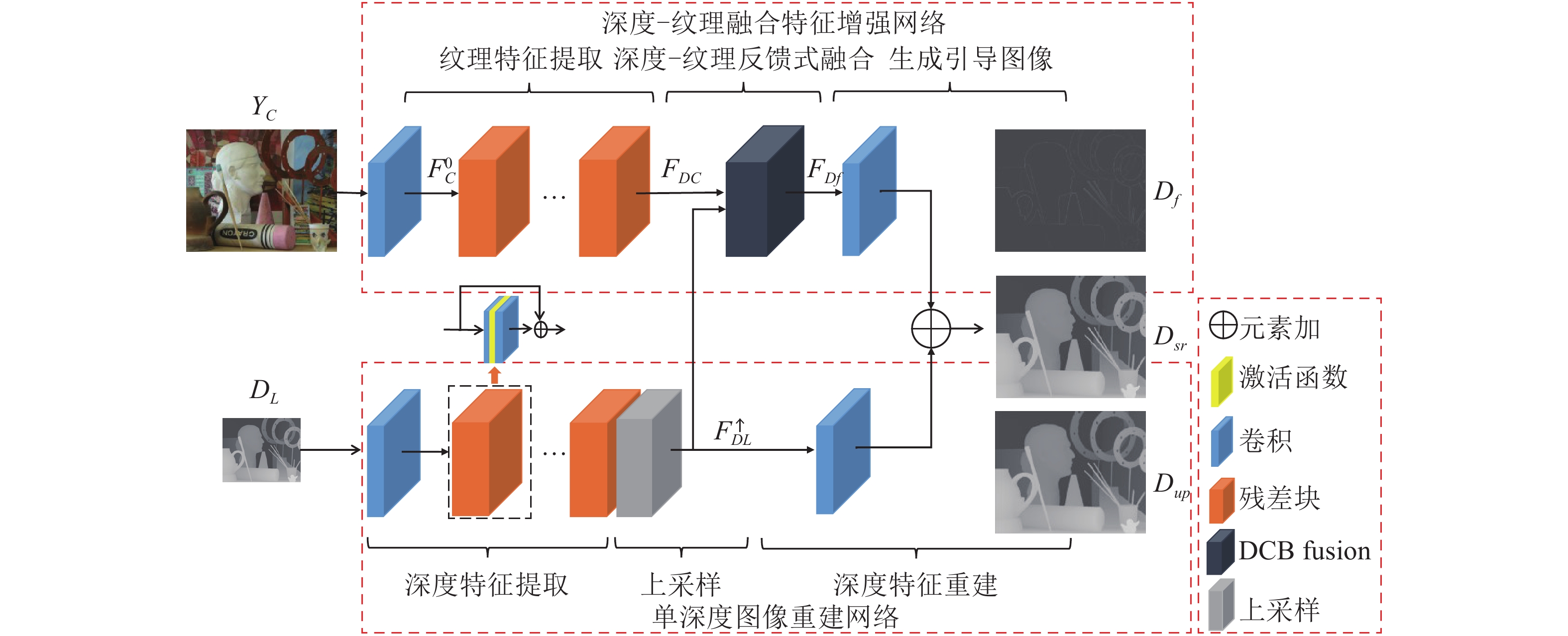
摘要: 受采集装置的限制, 采集的深度图像存在分辨率较低、易受噪声干扰等问题. 本文构建了分级特征反馈融合网络 (Hierarchical feature feedback network, HFFN), 以实现深度图像的超分辨率重建. 该网络利用金字塔结构挖掘深度−纹理特征在不同尺度下的分层特征, 构建深度−纹理的分层特征表示. 为了有效利用不同尺度下的结构信息, 本文设计了一种分级特征的反馈式融合策略, 综合深度−纹理的边缘特征, 生成重建深度图像的边缘引导信息, 完成深度图像的重建过程. 与对比方法相比, 实验结果表明HFNN网络提升了深度图像的主、客观重建质量.Abstract: Due to the limitations of the depth acquisition devices, the depth maps are easily distorted by noise and with low resolution. In this paper, we propose a hierarchical feature feedback network (HFFN) to reconstruct depth map with high-resolution. The HFFN uses a pyramid structure to mine the features of depth-texture at different scales, and constructs the hierarchical feature representations of depth-texture. In order to effectively utilize the structural information at different scales, a feedback fusion strategy based on hierarchical features is designed, which integrates the edge features of depth-texture to generate edge guidance information to assist the reconstruction process of depth map. Compared with the comparison methods, the experimental results show that the HFFN can achieve better subjective and objective quality.
-
Key words:
- Depth map /
- super-resolution reconstruction /
- feature fusion /
- residual learning
-
中国工程院近期在《走向新一代智能制造》一文中指出:新一代智能制造的技术机理是“人–信息–物理系统(Human-cyber-physical-systems, HCPS)”, 并指出新一代HCPS具备两个显著特征: 1)人将部分认知转移给信息系统, 因而系统具有“认知、学习”能力; 2)通过“人在回路(Humanin-the-loop)”的混合增强智能, 可极大地优化制造系统的性能[1].
人–信息–机器人融合系统(Human-cyberrobot-systems, HCRS)是HCPS在机器人领域中的具体应用.与之相应, 基于机器人的制造系统需要适应新一代智能制造的发展趋势.传统人机隔离生产方式刚性作业, 无法完成复杂多变生产任务, 也逐渐无法满足产品多品种、短周期、少批量、个性化的需求.而在HCRS中, 新型人机共融作业模式将人的优势(智慧性、灵巧性)与机器人优势(高速率、高精度、顺从性)高效结合, 实现人、信息与机器人系统的深度融合. HCRS具备HCPS的典型特征, 突出了人的中心地位, 将人的特点(包括灵巧性和应变能力)纳入到系统之中, 增强系统的智能程度, 可适应新一代智能制造过程中柔性、高效等要求.
其中, 人–机器人技能传递(Human-robot skill transfer, HRST)是HCRS中的关键之一, 是实现人与机器人的运动信息深度融合的基础. HRST的研究始于上个世纪80年代, 最近10年得到了很大发展, 目前是国际机器人领域中研究热点之一. HRST在不同文献中有不同称谓, 如示教编程(Programming by demonstration, PbD)、机器人示教学习(Learning from demonstration, LfD)、模仿学习(Imitation learning)等, 但其本质相同:人将自己的技能做通用化描述后传递给机器人, 进而实现机器人的运动编程, 可代替传统的机器人编程方式.机器人除了直接模仿人的技能外, 还可根据任务情况对所学技能进行泛化、拓展. HRST突出了人的因素在HCRS中关键作用, 可实现人机各自作业优势的结合, 适应人机共融协作要求.相比传统方式, HRST有诸多优势(见表 1).
表 1 HRST与传统方式的比较Table 1 Comparation between HRST and the conventional methods传统编程方式 人机技能传递 交互方式 人机隔离 共融交互 交互感受 编程不直观 自然、直观 编程人员 需要专业工程师 不依赖专业人员 机器人平台 针对具体机器人平台 技能不受限于特定平台 工作空间 受限于作业环境 受限程度小 任务情况 任务具体、固定 适应于不同任务, 可优化 编程效率 效率低下, 耗时多 效率较高, 便于重配置 人–机器人技能传递以交互的方式进行.一方面, 人根据任务情况自主调节自身的运动特征, 如根据与环境交互情况而自适应地调节肢体位置, 刚度/力; 另一方面, 机器人的运动响应可作为反馈信息帮助示教者对其运动进行修正与完善.从机器人角度来看, 不止是简单地模仿人的点对点(Point-topoint)运动轨迹, 而是具有“学习、推理”能力, 能够对所学“知识”进行泛化, 如具有目标拓展、运动识别、安全避障等, 以满足不同的任务要求.人机技能传递侧重强调人的因素在提高机器人技能方面的作用, 因此其主要的关注点是如何对人和机器人的运动进行通用化的描述.
本文针对人机技能传递展开讨论, 主要关注机械臂的技能示教学习.文章组织如下:第1节介绍机器人通用的技能学习过程; 第2节阐述实现人机技能传递的主要方式; 第3节总结几种主要的技能建模方法; 第4节介绍机械臂仿人控制问题; 第5节给出目前研究不足与未来发展方向; 第6节总结全文.
1. 技能传递一般过程
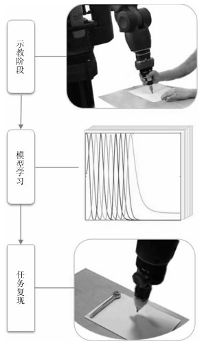
技能从人到机器人传递一般包括三个基本步骤: 1)示教阶段(Demonstration); 2)模型学习阶段(Model learning); 3)任务复现阶段(Task reproduction).以写字为例, 技能传递过程总体框图如图 1所示.
1) 示教阶段:在这一阶段, 示教者向机器人演示如何操作任务.这个过程可以是在线的, 也可以是离线的.在线是指在示教过程中, 机器人也跟随示教者操作任务, 记录下机器人在此过程中的运动信息的变化(包括位置、速度、力等信息)[2], 在此过程还可记录示教者肢体的刚度变化信息[3-4]; 离线示教是指在示教阶段, 只有示教者完成任务示范并记录下其运动状态变化, 而机器人在此阶段并不需要跟随示教者运动[5].
2) 模型学习阶段:在示教完成后, 获得了包含相应技能信息的数据集合.模型学习的主要作用是根据任务特点对示教的技能特征进行建模.利用示教数据拟合模型, 从而估计出模型参数.在此阶段, 除了需要考虑对运动轨迹表征(Representing), 还往往需要考虑多次示教轨迹对齐(Alignment)[6]、复杂技能的分割(Segmentation)[7]和运动拓展(Generalization)[8]等问题.
3) 任务复现阶段:在获得技能特征之后, 可将学习出的运动策略控制变量映射到机械臂的控制器中, 机器人可复现出示教者的技能, 甚至对其进行泛化, 以完成相应的作业任务.任务复现阶段需要选择合适的机械臂控制模式.控制模式可以是多样的, 根据任务要求可选择位姿控制、速度控制、力/力矩控制等.特别地, 对于与环境有敏感接触交互力的任务, 有效控制接触力是成功复现及泛化作业任务的关键因素.
2. 人机技能传递方式
人机交互接口设计(Interface design)是实现技能从人向机器人传递的首要环节, 决定了人通过何种方式对机器人进行示教.根据不同的交互接口, 常见的人机技能传递方式可归纳为以下三种形式:基于视觉的(Vision-based); 基于遥操作(Teleoperation-based); 人机物理接触交互(Physical human-robot interaction, pHRI).
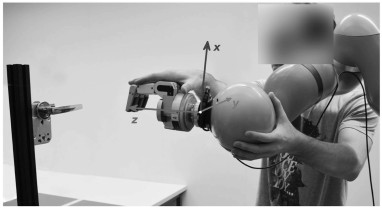
1) 基于视觉的人机技能传递[9-10].视觉输入是比较常用的运动示教方式.其基本原理是首先通过视觉设备(如三维体感摄影机Kinect、运动捕捉系统Vicon等)捕捉并跟踪人体运动信息并记录下来, 随后用机器学习算法对运动状态数据建模, 得到运动的通用化描述.最后在复现环节中, 根据具体任务特点, 泛化生成满足任务要求的控制指令.根据捕捉信息的特点又可将这种方法分为以下几种基本方法:利用Kinect相机[11]捕获示教者在运动时候手臂的关节角度, 再将人的关节角度映射到机器人的关节空间(Joint-space)[12-13], 如图 2(a)所示; 利用相机并结合光标(Optical marker)的方式, 光标可佩戴在示教者的手臂末端位置, 相机记录下手臂末端在示教过程中的运动轨迹, 进而将其映射到机器人的任务空间(Task-space)[5-6, 9], 如图 2(b)所示; 此外, 机器人还可以通过基于视频演示的方法学习到人的技能[14-15].
基于视觉的人机交互接口的优点是方便人的示教, 由于人的肢体不与机器人直接接触, 因而示教者的肢体运动可不受其限制.缺点是这种示教方式只能获取运动信息, 无法捕捉到人机接触情况下示教者的动作信息.另外, 由于示教者不能直接感受到交互力, 导致示教过程缺乏浸入感.
2) 基于遥操作方式的人机技能传递[16].通过遥操作的方式, 示教者可以通过主端(Master)设备操作从端(Slave)机器人.示教过程与基于视觉的方式很类似, 不同之处在于这种方式不再直接记录示教者的肢体的运动信息, 而是记录主端操作杆或者从端机器人的运动状态.由于操作杆与机器人的物理结构往往不同, 因而在示教过程中需要将二者的工作空间(Work space)进行匹配[17].目前, 遥操作已经被成功应用到了机器人辅助手术系统中, 如达芬奇手术机器人.
基于遥操作的示教方式的优点是可以用在远程操控场景与不适合示教者和机器人直接接触的工作场景中, 如核电辐射场所、对大型机器设备的示教编程等.其缺点是遥操作系统往往存在延时问题.另外, 震颤现象也是影响遥操作示教性能的重要因素之一[18].
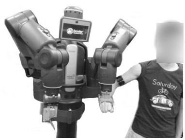
3) 基于物理交互方式的技能传递[19-20].所谓的物理交互是指示教者直接与机器人接触, 在机器人的示教模式下, 直接通过与机械臂的物理接触交互完成作业任务.该方式主要针对柔性协作机器人, 其机械臂具有一定柔性特性, 可以安全地与人协同作业, 一般提供了接口方便对其进行快速运动示教编程, 如图 4所示.
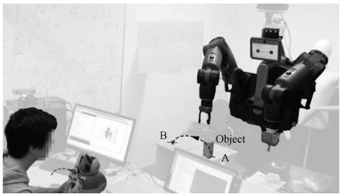
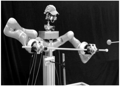
其中, 双臂示教是一种较为特别的物理交互示教方法[21-23], 即利用双臂机器人的特点, 以其中一机械臂为主端, 以另外一机械臂为从端.示教者操作主端引导从端机械臂完成作业任务, 如图 5.这种示教方式可以使得示教者直接操作机械臂, 有物理交互的特点.为了提高示教的质量, 可以在双臂示教系统中的主从两端引入基于虚拟阻抗的触觉反馈机制, 以提高人机交互的临场感[4].
3. 技能建模
3.1 运动表征问题描述
技能建模中需要解决的基本问题是如何实现对非线性运动(Nonlinear movement)的一般描述.任何复杂的行为都可以由简单的线性子系统的加权叠加来描述.可用以下公式来描述[26]:
$ \begin{equation} \dot{x} = \sum\limits_{i = 1}^{K} h_{i}(x, t)(A_{i}x+ b_{i}) \end{equation} $
(1) 其中, $ x $代表动作信息的特征变量, 如位置、速度、力等; $ h_{i} $表示各个线性子系统的加权系数, 而子系统$ f_{i} = A_{i}x+ b_{i} $由系数$ A_{i} $和$ b_{i} $确定.
由式(1)可知, 技能建模的关键在于确定上述的加权系数、估计子系统的参数以及选择合适的特征量.常见的基本建模方法包括动态运动原语(Dynamical movement primitives, DMP)、高斯混合模型(Gaussian mixture model, GMM)和隐马尔可夫模型(Hidden Markov model, HMM).
这几种模型的主要区别在于看待问题的角度不同: DMP把技能特征看作是运动原语(Primitive), 用示教数据拟合DMP模型可得到运动原语序列; 后两种是从概率角度看待技能示教与传递, 即把技能的各个特征与模型的不同状态(State)相对应, 用示教数据(对应概率语境中的观察数据, Observed data)拟合GMM或HMM模型.因此, 学习出模型的状态信息也就得到了相应的技能特征信息.
3.2 动态运动原语模型(DMP)
3.2.1 DMP基本数学描述
DMP模型[27-28]是由正则系统驱动的弹簧–阻尼系统来表示运动轨迹.原始DMP模型表示为[29-30]:
$ \begin{align} & \tau \dot{v} = \underbrace{K(x_g-x)-Dv}_{\text{线性部分}}+\underbrace{(x_g-x_0)f(s)}_{\text{非线性项}} \end{align} $
(2) $ \begin{align} & \tau \dot{x} = v \end{align} $
(3) $ \begin{align} & \tau \dot{s} = -\alpha_1 s \end{align} $
(4) 其中, $ K $, $ D $和$ \alpha_1 $是模型参数; $ x $和$ v $分别表示运动位置与速度; $ x_{0} $和$ x_{g} $表示运动轨迹的初始与目标. $ \tau $代表系统的时间常数, 决定系统的演化时间; $ s $代表系统的相位(Phase), 从1均匀收敛到0.
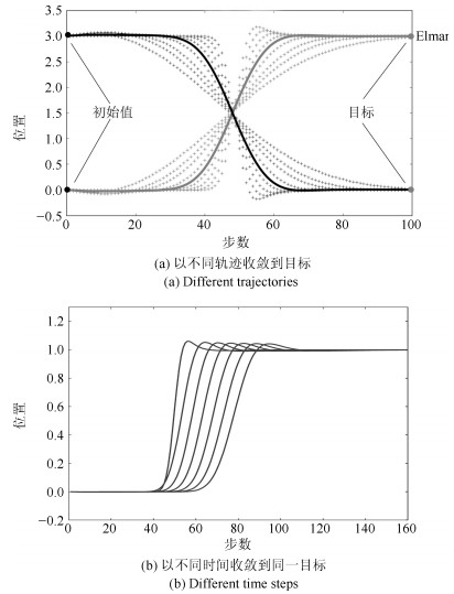
DMP模型本质上是一个二阶非线性方程, 包含两个部分:线性部分和非线性部分.以图 6(a)为例, 线性部分构成运动轨迹的基本形状(实线表示), 保证收敛到目标值; 非线性部分可将其调节成不同形状(虚线表示), 在保证形状相似性的前提下, 得到丰富的运动轨迹. DMP分为离散型(Discrete)和节律型(Rhythmic), 区别在于非线性项的核函数不同:前者为高斯核; 后者为余弦函数.这两种DMP分别用于学习点到点(Point-to-point)运动和具有周期性规律的运动[31].
可以用不同的非线性拟合方法逼近DMP模型中非线性项, 常用方法有局部加权回归算法(Locally weighted regression, LWR)和局部加权投影回归(Locally weighted projection regression, LWPR).通过DMP描述运动技能的的一个优点在于它的演化并不直接依赖于时间, 而是基于中间变量(即相位)的变化, 方便对运动轨迹进行拓展调节[28, 31].另外, 可通过对公式中初始位置、末端位置以及时间常数的调节来实现对运动轨迹在时间上或空间上的拓展与泛化(见图 6).
3.2.2 基于DMP的技能传递
目前, 学者在原始的DMP模型的基础上已经发展出了多个版本的DMP模型, 并应用于机器人技能示教学习. Ude等[32]不直接利用原有模型参数作为控制策略, 而提出了查询子(Queries)的概念来同时考虑任务参数与模型参数, 并可根据任务变化情况对其进行调节, 该方法在扔球(Ball throwing)实验上得到了很好验证. Muelling等[33]提出了一种DMP框架用来让机器人学习打乒乓球, 他们的框架考虑了以目标为中心(Goal-centered)的运动原语, 既考虑运动目标位置又考虑运动目标速度, 并可以同时对二者进行调节与拓展.
原始DMP模型有两个缺点: 1)当目标位置与初始位置很接近时, 则会产生很大的加速度, 这可能会损坏机器人本体, 也不利于协作者的安全; 2)如果拓展的位置目标相对于原始目标过零点(如从1拓展到$ -1 $), 则拓展的运动轨迹可能会相对于坐标轴发生翻转.为了克服这些问题, Hoffmann等[34]改进了原始DMP模型中的变换系统(Transform system), 提出了一种基于新的变换系统能够将外部物体位置信息耦合到该系统中, 可以实现实时在线避障, 通过Pick-and-place实验验证了他们的方法.
Rückert等[35]提出了参数化的动态原语模型(Parametrized DMP, PDMP), 将肌肉协同概念引入到该模型中, 用参数化的基函数替换原DMP中的径向基函数, 实验证明了其有效性. Krug等[36]提出了一种泛化的DMP模型(Generalized DMP, GDMP), 该模型把DMP的参数估计变成一个约束非线性最小二乘问题, 并把模型预测机制集成到示教系统中, 可以根据机械臂在当前运动状态下产生多种控制策略, 可起到意图预测、避障等作用. Meier等[37]提出了一种DMP的概率表示方法, 把该模型重构成带有控制输入的线性动态系统的概率模型, 方便直接将感知测量单元耦合到系统中, DMP系统可自动在线获取反馈信息, 并可根据似然估计结果对任务成败作出预判. Gašpar等[38]提出了弧长参数化的动态原语模型(Arc-length DMP, AL-DMP), 基本思想是将空间信息与时间信息分开表示, 可解决示教中存在较大运动速度差异的问题. Gams等[39]提出了适应于双臂交互的DMP模型, 基本做法是在两个DMP (分别用于机器人的左、右臂)的变换系统中耦合一对虚拟的相反作用力, 使得一只机械臂可以感知到另外一机械臂的位置与力的变化, 以达到良好的双臂协调控制效果(如图 7所示).
在人机示教过程中, 往往需要多次示教才能学习出好的控制策略, 而原始的DMP模型只能学习单一的示教轨迹.为了从多次示教数据中学习出技能特征, Yin等[40]用联合概率分布的方式替换了原有DMP模型中的归一化的径向基函数(Normalized radical basis function), 即将相位与非线性函数用联合概率分布表示, 再从多次示教数据中学习出一个非线性函数项, 便可以学习多次示教的结果. Matsubara等[41]提出了风格化(Stylistic)的动态原语模型(SDMP), 通过将运动风格(Style)信息耦合到DMP的转换系统中, SDMP可以同时描述多样化的运动轨迹, 达到了学习多次示教的目的, 该方法适合于多次示教数据差异较大的任务.
可以通过强化学习方法优化示教获得的运动原语.在人机示教技能传递的语境中, 强化学习方法的基本特征在于可实现对连续、高维原语空间的运动策略优化, 这区别于一般的强化学习方法.在技能复现阶段, 可以通过强化学习技术对变换系统中的非线性函数进行调节与优化[42], 按照一定目标来调节运动轨迹, 如按照最小加速度原则收敛到目标点、要求运动轨迹经过某些特定位置等. Kober等[43]将感知单元耦合到了DMP的系统中, 可以提高系统抵抗外部的干扰能力; 提出了一种基于权重探索的策略学习方法(Policy learning by weighting exploration with the returns, PoWER)对DMP学习到的控制策略进行优化. Theodorou等[44]提出了一种可应用于高维状态空间的算法, 即基于路径积分的策略优化方法(Policy improvement with path integrals, PI$ ^{2} $). Buchli等[45]将PI$ ^{2} $算法用于机器人技能学习, 用以优化运动原语模型参数. Li等[46]又将PI$ ^{2} $算法应用到了移动机器人的抓取操作上, 同时对机械臂与机械手关节空间进行轨迹优化, 取得良好的实验效果. Stulp等[47]利用PI$ ^{2} $算法用于机器人学习序列化的运动, 不仅优化模型参数, 还优化运动目标参数. Stulp等[48]又提出了一种进化策略方法(Evolution strategies, ES), 基本思想是将运动原语的演化调优看作是一个进化优化问题, 并通过数值仿真比较了PoWER、PI$ ^{2} $和ES的异同以及在同等条件下的收敛情况.
3.3 高斯混合模型(GMM)
3.3.1 GMM基本数学描述
GMM提出的时间比较早, 有很多变形版本, 已经被应用于诸多领域.我们只考虑在人机示教中对运动信息的表征情况.
在示教阶段获取的数据可以组合成数据对$ \lbrace\xi_{t}, z_{t} \rbrace_{t = 1}^{T} $.假设观测值$ \xi_{t} $是一个随机过程独立变量, $ z_{t}\in\lbrace 1, \cdots, K \rbrace $也相互独立.则其概率密度函数可表示为[49]:
$ \begin{align} & \mathcal{P} = \sum\limits_{i = 1}^{K}\pi_{i}f_{i}(\xi_{t}) \end{align} $
(5) $ \begin{align} & \sum\limits_{i = 1}^{K}\pi_{i} = 1 \end{align} $
(6) $ \begin{align} & f_{i}(\xi_{t}) = \mathcal{N}(\xi_{t}|\mu_{i}, \Sigma_{i}) \end{align} $
(7) 其中, $ \pi_{i} $表示第$ i $个高斯组分对应的系数; $ f_{i}(\xi_{t}) $是条件概率密度函数, 通常可表示成高斯分布$ \mathcal{N} $. GMM模型参数可概括成:
$ \begin{align} & \Theta_{\rm GMM} = \lbrace \pi_{i}, \mu_{i}, \Sigma_{i}\rbrace_{i = 1}^{K} \end{align} $
(8) 一般可以利用EM (Expectation-maximization)算法估计得到$ \Theta_{\rm GMM} $. GMM仅仅是用来对数据表征, 若要最终获得机械臂的运动控制策略, 还需要根据GMM模型参数生产运动控制变量.在机器人技能学习领域中, 高斯混合回归(Gaussian mixture regression, GMR)是实现这一目标的简单且高效的方法[50].例如, 控制变量$ \dot{\xi}^{*} $可以通过以下公式计算得到:
$ \begin{align} \dot{\xi}^{*} = &\sum\limits_{i = 1}^{K}h_{i}(x)\mathcal{P}(\dot{\xi}|\xi, i) = \\ & \sum\limits_{i = 1}^{K}h_{i}(s)[\mu_{i}^{\dot{\xi}} + \Sigma_{i}^{\dot{\xi}\xi}(\Sigma_{i}^{\xi\xi})^{-1}(\xi_{t}-\mu_{i}^{\xi})] \end{align} $
(9) 其中, $ h_{i}(x) $是归一化的权重, 上式中的参数即是由EM算法评估得到的GMM模型参数.
3.3.2 基于GMM的技能传递
近年来, 基于GMM模型的技能示教学习方法在文献中屡见报道.在算法方面, Muhlig等[51]将GMM模型引入到类人机器人的模仿学习框架中, 利用GMM学习到的运动信息, 可以根据目标物体的移动信息而动态调节相应的动作. Gribovskaya等[52]利用GMM模型来描述机器人运动中的多变量之间的关联信息, 能够在时间和空间扰动下快速重新规划机械臂路径. Khansari等[53]提出了一种利用GMM学习稳定非线性动态系统的方法, 可保证机械臂在接近目标位置时能够尽可能地跟随示教者的运动姿态, 这有利于机械臂可以更好地捕获示教者的运动信息. Cederborg等[54]提出了一种新的GMM模型(Incremental, local and online variation of Gaussian mixture regression, ILO-GMR), 相比于传统GMM模型, ILO-GMR将任务信息耦合到局部动态系统中, 能够使得机器人在线学习新的运动技能, 而不需要重复地调整模型参数, 在一定程度上提高了技能传递的效率.
Calinon等[55]提出了一种基于GMM的运动技能的示教学习框架, 能够同时处理关节空间与笛卡尔空间的任务限制, 并可使得机器人能够重复利用已经学习到的技能来处理新的任务情形. Calinon等[56]又提出了一种将任务信息参数化的混合模型(Task-parameterized mixture model, TP-GMM), 其核心思想是把模型参数与任务参数结合起来, 即把任务参数耦合到GMM模型中, 在任务复现阶段能够实时地调节参数化的轨迹以满足不同的作业任务要求. Alizadehl等[57]拓展了TP-GMM模型, 使之能够解决在示教阶段或者复现阶段中的部分任务参数信息缺失的问题. Huang等[58]对TP-GMM进行了优化, 选择直接优化任务参数而不是GMM的组分(Component), 这样将模型学习变成一个低维空间的优化问题, 并且设计了一种特征选择机制, 可以自动选出重要的任务帧(Task frame)而剔除不重要的任务帧.为了有效表征机械臂末端执行器在完成任务中的旋转特征, Zeestraten等[59]提出了在黎曼流形域中的GMM模型, 该方法能够有效表征机械臂在任务空间的位姿联合分布状态, 可使得机器人学习到示教者的更加丰富的技能特征.
在应用方面, GMM被应用于不同类型的作业任务以及不同的机器人平台上. Reiley等[60]将GMM应用到了机器人辅助手术任务中, 用GMM表征医生手术过程中的动作信息, 再将生成的控制策略传递给手术机器人.此外, Chen等[61]利用GMM模型把技能传递给柔性手术机器人. Wang等[62]将GMM模型应用到软体机器人的运动技能学习中, 用GMM表征示教数据并评估出执行器的合适路径, 在试验中取得了良好效果. Kinugawa等[63]者的运动意图, 并可以根据人的意图预测结果自适应地对装配任务进行任务规划, 达到了良好人机交互效果. Goil等[64]利用GMM模型解决辅助轮椅导航系统中人机混合控制问题, 将用户的控制命令作为任务限制耦合到运动学习过程中, 实验取得了良好人机协同控制效果.
3.4 隐马尔可夫模型(HMM)
3.4.1 HMM基本数学描述
在人机示教技能传递的语境中, 常用一阶HMM模型分析时间序列.给定一个状态序列$ \lbrace{s_{1}, s_{2}, \cdots, s_{T}}\rbrace $, 可用以下公式表示其其联合分布[65]:
$ \begin{align} & \mathcal{P}(s_{1}, s_{2}, \cdots, s_{T}) = \mathcal{P}(s_{1})\prod\limits_{t = 2}^{T}\mathcal{P}(s_{t}|s_{t-1}) \end{align} $
(10) 并且假设当前状态只与上一时刻状态有关, 即:
$ \begin{align} &\mathcal{P}(s_{t}|(s_{t-1}) = \mathcal{P}(s_{t}|s_{1}, s_{2}, \cdots, s_{t-1}) \end{align} $
(11) 与GMM模型参数相对应, HMM模型参数可表示为:
$ \begin{align} & \Theta_{\rm HMM} = \lbrace \lbrace a_{i, j}\rbrace_{j = 1}^{K}, \pi_{i}, {\mu}_{i}, {\Sigma}_{i} \rbrace_{i = 1}^{K} \end{align} $
(12) 其中, $ a_{i, j} $为状态转移矩阵中的元素. HMM的参数可用前向–后向算法(Forwar-backward)或者EM算法估计得到.与GMM类似, 在用HMM对示教数据建模后, 也需要利用回归算法生成机器人的运动控制命令.
在GMM模型中, 状态之间相互独立, 状态之间的转移与时间信息无关; 和HMM模型中, 状态驻留概率为均匀分布.因此, GMM模型和HMM模型不能很好地表征运动技能的时间信息.而隐半马尔科夫模型(Hidden semi-Markov models, HSMM)用高斯函数表示HMM中的状态驻留概率, 可以改善HMM在表征时间信息的性能.相应地, HSMM的参数可表示为:
$ \begin{align} & \Theta_{\rm HSMM} = \lbrace \lbrace a_{i, j}\rbrace_{j = 1, j\neq i}^{K}, \pi_{i}, {\mu}_{i}, \mu_{i}^{d}, \Sigma_{i}^{d}, {\Sigma}_{i} \rbrace_{i = 1}^{K} \end{align} $
(13) 其中, $ {\mu}_{i} $和$ \mu_{i}^{d} $分别表示第$ i $个状态的均值与方差. 图 8反映了在两个状态下GMM, HMM与HSMM建模示例以及三者之间的主要区别.
3.4.2 基于HMM的技能传递
Asfour等[66]将HMM模型引入到类人机器人的模仿学习中, 用示教数据中的关键特征来训练HMM模型, 实验表明相对于GMM, HMM可以很好地反映出机器人双臂之间在完成任务过程中的时间关联性. Calinon等[67]提出了一种基于HMM-GMR模型的架构使机器人可以学习人的运动技能, 用HMM对人体运动信息建模, 用GMR做回归得到机器人的运动控制命令.该架构与GMM-GMR类似, 但可以表征更加丰富的运动信息, 该算法具有更强的鲁棒性.
Vuković等[68]首次将该方法应用到移动机器人的示教学习中, 用HMM对机器人的移动信息建模, 试验证明了其有效性. Medina等[69]结合HMM模型和线性参数变化(Linear parameter varying, LPV)系统, 提出了HMM-LPV模型, 用HMM对复杂任务建模, 用LPV保证HMM每一个状态或子任务(Subtask)的稳定性, 该模型可以学习序列化的、与时间变化无关的运动控制策略.
Hollmann等[70]提出了一种基于HMM的机器人示教编程方法, 通过对机器人的运动控制信息添加约束, 使得机器人可以自动地根据人的运动特征做出相应的反应, 并在一家金属加工公司的生产线上验证了所提方法. Vakanski等[6]提出了一种机器人运动轨迹学习方法, 用HMM表征示教轨迹, 并通过在状态转移时设置关键点(Key points)的办法, 实现对轨迹的拓展与调整, 在刷漆(Painting)作业中验证了该方法的有效性. Rafii-Tari等[71]提出了一种基于分层级的(Hierarchical HMM, HHMM)模型以应用于机器人辅助血管内导管插入术.他们把该手术任务分成多个序列化的运动原语, 用HHMM模型分别对各个原语状态以及它们之间的关联信息建模, 可以使得机器人对协作者的运动输入有一定识别和预测能力.
如前文所述, HMM无法表征每个状态的驻留时间.为此, Calinon等[26]将HSMM引入到机器人示教学习中, 利用HSMM同时对时间信息和运动信息建模, 即保留了HMM模型的优点, 又能提高抗干扰能力, 尤其在时间域上的抗干扰能力. Pignat等[72]利用HSMM表征人机协作场景中的感知信息与运动控制信息, 即把协作者的运动与机器人的运动在空间位置与时间上都关联起来, 机器人可以根据人的当前运动状态而做出在空间域与时间域上的运动响应, 该方法被应用到了机器人辅助穿衣任务. Rozo等[73]进一步提出了可自适应调节每个状态持续时间的HSMM模型(Adaptive duration hidden semi-Markov model, ADHSMM).与传统的HSMM模型相比, 不再用固定的高斯分布来表征其状态驻留时间, 而是可以根据与环境交互情况自适应地调节, 因而ADHSMM对运动的时间信息具有更强的表示能力, 具有更强抗外部干扰能力.
DMP、GMM、HMM三种模型比较:由于模型差异, 难以对三者细致比较.总体来说, DMP具有模型简洁, 计算效率高, 泛化能力强的优点, 但DMP独立表征各运动维度信息, 丢失了各维度之间的关联信息.例如, 当用DMP模型对机械臂末端运动位置与交互力建模时, 只能对力与位置分别建模与描述, 就无法表征出位置与力的关联信息, 可能会导致信息丢失而不能很好地学习到示教者的运动.另外, 在模型学习阶段需要提前选择离散型DMP或节律型DMP[24].而GMM和HSMM可以表达出各维度的关联信息, 但模型复杂, 计算效率相对较低, 通常需要较长的时间学习模型参数. HSMM可以反映各个状态之间的转换信息, 因而比GMM具有更强的运动信息表达能力, 但在同等条件下需要更长的计算时间[26]. 表 2总结了这三种模型与其常见变种模型的的基本特点, 以及利用它们学习到的技能示例.
表 2 DMP、GMM、HMM模型特点总结Table 2 The summary of DMP、GMM、HMM models模型 常见变种 基本特点 技能示例 DMP - 模型简单; 拓展性好; 学习单次示教; 计算效率高$^{1}$. Tennis swings[75] Bio-inpisred DMP 可以克服跨过零点问题, 可在线动态避障. Pick-and-place[34] PDMP 适用高维$^{2}$、连续系统; 对多种运动灵活表达. Walking[36] GDMP 可实现多种控制策略, 起到意图预测等作用. Grasping[37] AL-DMP 空间与时间信息分别表示, 更好地表达运动速度. Reaching positions[39] SDMP 可从多次差异较大的示教结果中学习技能特征$^{3}$. Table tennis[41] ProMP$^{4}$ 对运动原语概率化表示; 可有机混合不同运动原语. Robot hockey[76] Coupling DMP 耦合双臂运动信息, 适宜双臂、协作操作任务. Bimanual tasks[35] DMP-based RL 通过强化学习方法对DMP轨迹优化. Ball-in-a-cup[43] GMM - 可表达不同维度的关联信息; 可表征多次示教; 计算效率相对低. Gripper assembly[77] ILO-GMM 局部耦合运动信息; 增量学习运动技能. Moving[54] TP-GMM 耦合任务参数到模型中; 对参数化轨迹在线调节. Rolling out a pizza[56] TP-GMM on RM$^{5}$ 用黎曼流形表示GMM, 有效表达末端位姿分布信息. Bimanual pouring[59] HMM - 相比GMM对运动的信息表达能力更强; 计算效率相比较低. Ball-in-box[78] HMM-GMR 用GMR做回归模型, 可在线生成运动控制命令; 鲁棒性好. Feeding[67] HMM-LPV 保证每个子状态的稳定性, 适宜复杂任务建模. Reach-Peel-retractg[69] HSMM 可表达状态驻留时间, 相比HMM抗外界干扰能力强. Button pushing[12] ADHSMM 自适应调节状态驻留时间, 对时间信息表达能力更强. Pouring[73] 1 计算效率高是指离线下模型学习时间短, 这里不包括基于DMP的强化学习算法.
2 指对多个自由度个数, 如对7-DOF的机械臂同时学习位置与速度, 则维度为14.
3 指多次示教的轨迹重合度小, 难于对齐, 如打乒乓球时的运动轨迹.
4 概率化运动原语(Probabilistic movement primitives, ProMP).
5 指黎曼流形(Riemannian manifolds, RM).3.5 建模中的其他问题
在建模阶段, 除了需要考虑对运动做通用化描述外, 还有一些问题需要考虑, 主要包括: 1)轨迹对齐(Alignment)问题; 2)技能分割(Segmentation)问题.
1) 轨迹对齐问题
由于示教的差异, 多次示教的运动轨迹往往在时间轴上长短不同, 在空间上也会有一定差异, 这种差异有时候还会比较大, 影响模型学习结果.为了达到更好的运动技能学习效果, 需要对示教数据进行对齐处理.动态时间规整(Dynamic time warping, DTW)是常用的对齐数据的技术, 在机器人技能学习领域应用广泛. Muhlig等[51]在用GMM对示教数据建模之前, 用DTW在时间上对运动轨迹进行了对齐处理. Vakanski等[6]结合HMM与DTW技术, 利用DTW对运动轨迹的关键点进行对齐, 实验证明该方法要比没有对齐的情况获得更好的效果.为了对齐人机协作场景中示教者与机器人的运动轨迹, Amor等[74]把DMP与DTW模型结合起来, 利用DTW把人与机器人的各自运动相位变量对齐, 这样二者的运动内部信息便可关联起来, 人机双方的运动便能够得以协调起来, 该方法比较适合人机协作的作业任务.
2) 技能分割问题
技能分割主要针对以下情况: a)复杂的任务往往包含多个步骤, 其运动轨迹的动态特征非常复杂, 用上述三种模型对其整体运动轨迹一次性建模比较困难; b)对于序列化的运动轨迹, 经常需要分阶段拓展, 即轨迹拓展的目标不止一个, 因而需要分段处理; c)在机器人复现任务过程中, 对其分阶段添加不同的限制, 需要机器人在各阶段作出不同的响应.面对这三种情况, 技能(或任务、轨迹)分割是解决问题的有效办法.基本思想简单、直接:把作业任务分割成多个阶段, 用上述模型对分割后的各个运动片段(Segments)分别建模, 再针对每一阶段具体情况分别考虑.
目前, 关于技能分割的文献报道较少, 主要有以下几种方法. Fox等[79]提出了$ \beta $过程自回归隐马尔科夫模型(Beta process autoregressive HMM, BP-AR-HMM), 用于分割连续的人体运动. Niekum等[80]对BP-AR-HMM进行了改善, 将其应用到机器人示教学习领域, 把BP-AR-HMM与DMP结合形成了一个完整的示教学习框架, 前者用于分割; 后者用于表征.随后, Chi等[81]将这一框架应用到了安装在轮椅上的机械臂示教学习中, 实验取得了良好效果. BP-AR-HMM算法的优点是全自动分割, 不需要先验设置分割的片段数量; 缺点是鲁棒性差, 容易导致过分割的情况.
最近, Lioutikov等[82]提出了一种概率分割(Probabilistic segmentation, ProS)方法, 该算法是基于对DMP的概率表示[38], 在对轨迹建模的同时完成技能的分割.在同等条件下, ProS比BP-AR-HMM具有更强的鲁棒性, 可获得更好的分割效果.但ProS是一种半自动的分割方式, 需要先验设置分割数量.
4. 仿人自适应控制
机械臂的仿人控制是一个很大的范畴, 一直得到了广泛的关注与研究.在人机技能传递领域, 仿人控制具有比较明确的目标与意义.这里的仿人控制是指如何借鉴人的手臂灵活的操作能力, 来实现机械臂的灵巧控制, 或者说如何实现将人手臂的自适应控制模式传递给机械臂.
4.1 人体神经肌肉运动控制机理带来的启示
对于雕刻这样的任务, 机器人难以胜任, 而人却可以比较轻松地完成.学者对了解人类是如何拥有灵巧的操作能力表现出了浓厚的兴趣, 在探究人体神经肌肉运动控制机理方面展开了大量研究. Schweighofer等[83]展示了小脑能够补偿人的手臂与外界的相互作用力矩, 进而通过学习部分逆动态模型而改进预先存储在运动神经元皮层的基本逆动态模型, 从而在目标定向运动中提高精确度, 又进一步将人体肌肉的同步收缩解释为一种不受时延影响的分布式的局部控制策略, 表明主动改变系统刚度的能力可以克服反馈滞后的缺点.
特别地, Shadmehr等[84]在运动神经元控制方面的研究中发现共同收缩(人改变内在的肌肉–骨骼刚度的能力)在处理不确定性和不可预测性方面起到了关键性作用. Burdet等[85]证实了人的手臂具有一种类似弹簧的性质, 在中枢神经系统(Central neural system, CNS)的控制下, 手臂可以自适应地调节阻抗/刚度以适应任务的变化, 当外部环境变化时, 手臂能够自然地增加阻抗以提高抗干扰能力, 而当不需要高刚度时, 又能够自然地降低刚度. Mitrovic等[86]研究表明中枢神经系统可以通过适当的主动肌/对抗肌的同步收缩来控制手臂平衡, 并研究证实了共同收缩在处理不确定性最小化方面具有重要作用.
上述研究成果表明人的这种变阻抗/刚度控制能力是完成灵巧作业任务的关键, 这对于实现机械臂的灵巧控制、改善机器人的操作技能具有重要启示作用.近年来, 人机示教领域的学者开始关注于如何使机器人学习自适应变刚度控制策略.这些方法基本可以分为两类: 1)基于学习的变刚度控制方法; 2)人机变刚度控制策略传递.
4.2 基于学习的变刚度控制方法
阻抗控制是实现力控的常用方式, 一个典型的关节阻抗控制器可用以下公式表示:
$ \begin{equation} \begin{aligned} \tau_{cmd} & = K^{P}(x_{des}-x_{cur})+K^{D}(\dot{x}_{des}-\dot{x}_{cur}) +\\ & \tau_{for}+\tau_{dyn}(x, \dot{x}, \ddot{x}) \end{aligned} \end{equation} $
(14) 其中, $ \tau_{cmd} $是控制输入力矩, $ \tau_{for} $是前馈项, 用于补偿机械臂与外界的交互作用力, $ x_{des} $和$ x_{cur} $分别代表目标关节角度和当前的关节角度, $ \tau_{dyn} $用以补偿系统的动态力如重力和科里奥利力等. $ K^{P} $和$ K^{D} $分别表示刚度与阻尼, 通常阻尼项设置为$ K^{D} = \lambda \sqrt{K^{P}} $, $ \lambda $是预设常值.变阻抗控制的目标是适当地调节刚度值, 以达到提高机械臂柔性的目的[87-90].
基于学习的方法实现机械臂的变刚度控制是指通过学习技术(如强化学习)来对刚度轨迹进行调节, 获得适当的变刚度控制策略. Buchli等[45]提出了一种基于强化学习的方法来调节刚度轨迹.其基本思路是利用DMP模型变换系统的最后一项即非线性项(参见式(2))来表示刚度, 再用PI$ ^{2} $算法对这一非线性优化, 通过设置一个合适的代价函数, 最终可以得到变化的刚度轨迹.该算法用一固定的初始值拟合PI$ ^{2} $算法, 因此收敛速度与初始值的选择有很大关系, 通常需要很长的训练时间和较多的训练次数.
Steinmetz等[89]提出了一种基于DMP的方法来实现力控, 他们的主要思路与Buchli的方法相似, 不过没有直接利用强化学习技术来优化非线性项, 而是设计了一种刚度值选择机制来调节刚度, 例如当机械臂在运动过程中把刚度设定一个较高值, 而当与外部环境接触, 将刚度设定为零.他们的方法不需要很长的学习时间, 但不能连续调节刚度值.
Rozo等[90]提出了一种基于HMM-GMR的方法来学习变刚度轨迹.其基本思路是在示教阶段, 同时记录位置信息与力信息.在建模阶段, 用联合概率分布来同时表示位置与力, 学习后的HMM模型就能够表征力的变化信息, 再通过以下公式将力与刚度联系起来:
$ \begin{align} F_{t} = \sum\limits_{i = 1}^{N}h_{t, i}[K^{P}(\mu_{n, t}^{x}-x_{t})] \end{align} $
(15) 其中, $ \mu_{n, t} $是HMM模型第$ n $个状态在时间$ t $时候的位置均值, $ h_{t, i} $是状态的权重(参见式(9)).通过式(15)可以获得变刚度轨迹, 并且可以反映出相应的力的变化情况.
受此启发, Racca等[24]进一步利用HSMM-GMR模型来学习刚度, 用HSMM模型替换HMM模型可以提高系统对外界的抗干扰能力, 这对于接触型(In-contact)任务十分有利.并且, 他们还将机械臂末端的旋转力矩信息耦合到HSMM模型中, 因而还可以学习出旋转刚度轨迹, 即实现了在旋转方向上的变刚度调节.
4.3 人机变刚度控制策略传递
上述的学习刚度的方法都需要在一个学习过程才能够获得刚度轨迹, 显然不够直接, 并且很难准确反应人体的刚度变化特征.另外, 在这些方法中刚度是通过基于力计算得到的, 往往需要额外的传感器测量力, 增加整体机器人系统的成本.更加直接的方式是人机变刚度控制策略传递, 即在人机交互过程中, 提取人的肢体刚度变化特征, 将其直接传递给机械臂, 以达到变刚度控制的目的.
研究者们发现利用人体生理肌电信号(Eletromyography, EMG)可以实现人手臂到机械臂的力传递策略.肌电信号是运动单位产生的动作电位序列(Motor unit action potential trains, MUAPT)在皮肤表面叠加而成的一种非平稳微弱信号, 由中枢神经系统进行调节控制, 表征了肌肉的伸缩以及关节力度和刚度变化等信息, 因而EMG信号与肌肉力度/刚度的调节、运动意图等具有很大的关联性.肌电信号使得我们能够从生理层次提取运动肌肉控制特性, 弥补传统的示教技术仅从物理层次上实现人机交互的不足.
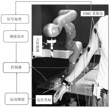
近些年来, 机器人领域的学者开始利用EMG信号提取人的肢体刚度特征, 并用于控制机械臂. He等[88]提出了一种基于EMG信号的变阻抗遥操作系统, 如图 9所示, 根据EMG估计出人的手臂刚度, 人在视觉反馈下调节手臂刚度, 并传递给机械臂, 实现机械臂的自适应柔性控制. Ajoudani等[11]又提出了一种基于扰动测量的手臂刚度简化的评估方法, 通过肌肉共收缩情况定义一个刚度指示器, 其变化可反映出人体肌肉活化程度, 该方法可实现基于EMG信号实时估计出人体刚度. Yang等[4]进一步将触觉反馈机制引入到该类系统中, 同时在触觉和视觉反馈的帮助下, 人可以更加自然地示教, 增加了技能传递的临场感.
Liang等[3]提出了一种人体刚度增量估计算法, 利用刚度与力增量之间的线性映射关系, 估计出肢体刚度系数, 这种方式可以忽略掉EMG信号的非线性残差, 他们通过教授机器人写字, 证明了该算法的有效性. Li等[92]进一步利用该方法估计人体刚度, 并将其用于控制上肢外骨骼机器人, 可实现外骨骼自适应地调节刚度, 取得了良好实验效果.
Howard等[93]比较了在不同层级上将人的行为传递给变阻抗驱动器(Variable impedance actuators, VIAs), 主要分析了基于EMG信号的人体阻抗调节特征的传递, 指出特征传递比直接动作模仿具有更好效果, 他们的结论可提供很好的借鉴作用. Peternel等[94]提出了一种人机协作系统, 如图 10所示, 将人的手臂刚度与机械臂的刚度协调起来, 机械臂的刚度由示教者的手臂刚度的变化决定.例如, 当在一个拉锯任务场景中, 当人拉锯时增大手臂力度, 机械臂就减小刚度处于松弛状态, 反之亦然, 这种方法适合于人机协同调节交互力的任务场景.
在上述的刚度传递过程中, 大多只关注于将评估出的人体刚度轨迹直接映射到机械臂的控制器中, 而对刚度的动态特性分析不足. Yang等[25, 95-96]提出了一种人机示教框架, 将运动轨迹与刚度轨迹等同看待, 提出用统一的框架对二者分别建模, 这样可实现运动特征与刚度特征从人向机器人的同时传递, 获得更加完整的技能传递过程.并且, 他们的方法可学习多次示教刚度轨迹, 保留对空间位置与刚度分别调节的空间, 可实现对二者同时或者分别拓展与分割, 有利于提高机器人的技能学习能力.
上述刚度传递的一般过程是:先离线估计出示教者手臂末端的刚度, 再映射到机械臂的末端工作空间, 最后通过逆运动学作用到关节力矩控制器. Fang等[97]利用零关节空间刚度特性, 开发了基于模型的人体关节空间估计方法, 实现在线在多个位置和不同程度的肌肉活化度下对手臂7个关节的刚度估计, 该方法有望实现人机关节空间的刚度直接传递, 提高变刚度自适应控制的效率.
5. 问题与展望
综上所述, 人机技能传递技术虽然取得了一定进展, 但仍然存在多个方面问题.主要体现在:
1) 在人机技能传递方式方面, 目前的交互方式过于单一、感知信息不足, 人机融合程度不高, 造成示教的浸入感不足, 示教者缺乏比较真实的临场感, 从而影响示教性能.
针对这一问题, 未来会集中在寻求更加直观、自然、友好的示教方式.首先, 在人机交互接口上, 多种交互方式相结合是发展趋势, 将先进的交互技术引入到机器人技能示教学习领域是确实可行的办法, 例如, 利用虚拟现实(VR)、混合现实(MR)以及三维再现等技术[98-101]构建人机示教交互与作业环境, 有望缩小人机隔离状态, 达到更好人机共融效果, 可提高示教质量.
多模态信息融合也将是改善人机交互性能的发展方向.通过将物理的或者生理的多种形式的信号(如空间位置、交互力、触觉、视觉、肌电信号等)在更高层次上融合, 纳入到人机技能传递过程中, 可以更直观地表达出人的技能特征.
2) 在技能建模、学习方面, 目前所用的模型大多是传统的机器学习模型, 泛化能力不足, 使得机器人学习技能过程在很大程度上受到具体示教场景、示教者本身、作业环境等诸多因素的制约.
结合示教学习和深度强化学习等技术是解决这一问题的有效方式之一.近年来, 人工智能技术在机器人视觉感知、技能学习等方面展现出较大的应用潜力[102-105].虽然现有的基于人工智能的机器人技能学习方法侧重于机器人自主提升技能, 与人机示教技能传递存在很大差别, 但人工智能有望作为一种辅助技术手段以提高人机示教的性能.一种思路是先利用示教技术使机器人具备一定的类人化的操作技能, 再通过深度强化学习提高机器人的技能泛化能力.例如, 可考虑如何用深度强化学习技术优化运动原语控制策略.
3) 在机械臂控制方面, 虽然目前可以实现人体刚度特征向机器人的传递, 但对人体刚度调节机制理解不够深入, 人手臂与机械臂在结构上具有差异性, 影响刚度评估的准确性.刚度估计方法也繁琐复杂, 影响技能学习效率.
为了进一步理解肌肉活化、信息感知、运动控制等内容, 有必要深入探究人体的运动机理.更好地理解人体肌肉模型, 开发具有普适应的刚度估计方法.从人类的运动控制中汲取经验, 是未来提高机器人类人化操作能力的重要研究方向[106].
6. 结束语
本文主要介绍人机技能传递取得的研究进展.首先, 阐述了机器人技能学习在新一代智能制造时代的研究背景, 尤其是与HCPS之间的关系.介绍了技能传递一般过程:示教–建模–技能复现, 以及几种主要的人机技能传递方式, 并分析了各自的优缺点.接着阐述了三种基本的技能建模模型: DMP、GMM、HMM, 以及它们的主要变种, 总结了各自的特点.接着, 介绍了两种实现机械臂变刚度控制的方式:基于学习算法和人机刚度特征传递, 并分析了各自的优缺点.最后, 总结了示教学习在三个方面面临的主要问题、现阶段不足之处, 并给出了可能的解决之道与未来发展方向.
在过去的十年里, 人机技能传递技术得到了较快发展, 无论是在人机接口设计与建模, 还是在仿人手臂自适应控制上都取得了一些可喜的成果.但有诸多不足, 与达到应用的地步还有一段距离.人机技能传递是个典型的交叉学科问题, 需要机器人学、控制、机器学习、神经科学等多个学科的研究人员共同努力, 才能推动其不断进步, 最终走向工业界.
目前, 我国在此领域处于刚刚起步阶段, 相关成果报道很少, 离国际先进水平有很大的差距, 需要国内学者加倍努力, 在理论与技术上都有所建树, 争取早日把人机示教技术推向应用, 助力我国智能制造业发展.
-
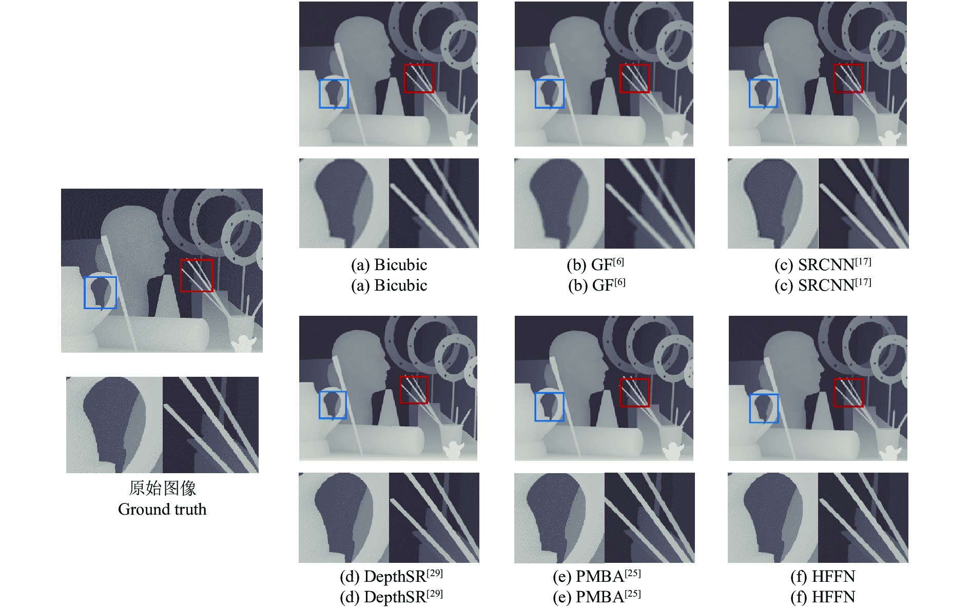
图 6
$ 4\times $ 尺度下测试图片“Art”的视觉质量对比结果Fig. 6 Visual quality comparison results of “Art” at scale
$ 4\times $ 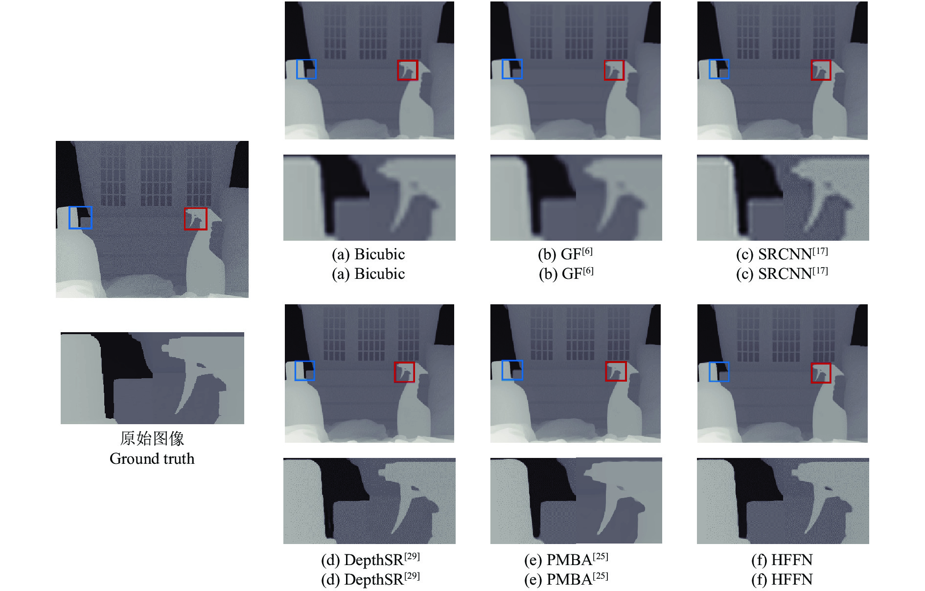
图 7
$ 8\times $ 尺度下测试图片“Laundry”的视觉质量对比结果Fig. 7 Visual quality comparison results of “Laundry” at scale
$ 8\times $ 表 1 残差块数目对HFFN网络性能的影响
Table 1 Influence of the number of residual blocks on the performance of HFFN
网络模型 H_R3 H_R5 H_R7 H_R10 训练时间(h) 3 3.8 4.4 5.4 模型参数(M) 2.67 2.96 3.26 3.70 重建结果(dB) 48.14 48.23 48.45 48.54  下载: 导出CSV
表 2 金字塔层数对HFFN网络性能的影响
Table 2 Influence of pyramid layers on the performance of HFFN
网络模型 H_P2 H_ P3 H_ P4 训练时间(h) 3.6 3.8 8.6 模型参数(M) 1.62 2.96 8.34 重建结果(dB) 48.04 48.24 48.32
下载: 导出CSV
表 3 消融分析结果
Table 3 Results of ablation study
网络 纹理 分层 深层 融合 结果(RMSE/PSNR) Basic $ \checkmark$ 3.2238/40.071 H_Color $ \checkmark$ $ \checkmark$ 2.8239/41.438 H_CP $ \checkmark$ $ \checkmark$ $ \checkmark$ 2.8544/41.578 H_Res $ \checkmark$ $ \checkmark$ $ \checkmark$ 2.9352/41.285 HFFN-100 $ \checkmark$ $ \checkmark$ $ \checkmark$ $ \checkmark$ 2.7483/41.671
下载: 导出CSV
表 4 测试数据集A的客观对比结果 (RMSE)
Table 4 Objective comparison results (RMSE) on test dataset A
对比算法 Art Books Moebius $ 2\times $ $ 3\times $ $ 4\times $ $ 8\times $ $ 2\times $ $ 3\times $ $ 4\times $ $ 8\times $ $ 2\times $ $ 3\times $ $ 4\times $ $ 8\times $ Bicubic 2.66 3.34 3.90 5.50 1.08 1.39 1.63 2.36 0.85 1.08 1.29 1.89 GF[6] 3.63 3.84 4.14 5.49 1.49 1.59 1.73 2.35 1.25 1.32 1.42 1.91 TGV[14] 3.03 3.31 3.78 4.79 1.29 1.41 1.60 1.99 1.13 1.25 1.46 1.91 JID[16] 1.24 1.63 2.01 3.23 0.65 0.76 0.92 1.27 0.64 0.71 0.89 1.27 SRCNN[17] 2.48 3.05 3.71 5.28 1.03 1.26 1.58 2.30 0.81 1.03 1.23 1.84 Huang[21] 0.66 / 1.59 2.71 0.54 / 0.83 1.19 0.52 / 0.86 1.21 MSG[25] 0.66 / 1.47 2.46 0.37 / 0.67 1.03 0.36 / 0.66 1.02 RDN-GDE[26] 0.56 / 1.47 2.60 0.36 / 0.62 1.00 0.38 / 0.69 1.05 MFR-SR[27] 0.71 / 1.54 2.71 0.42 / 0.63 1.05 0.42 / 0.72 1.10 PMBA[28] 0.61 / 2.04 3.63 0.41 / 0.92 1.68 0.39 / 0.84 1.41 DepthSR[29] 0.53 0.89 1.20 2.22 0.42 0.56 0.60 0.89 / / / / HFFN 0.41 0.84 1.28 2.29 0.28 0.37 0.49 0.87 0.31 0.45 0.57 0.89 HFFN+ 0.38 0.81 1.24 2.19 0.27 0.36 0.47 0.84 0.30 0.44 0.55 0.85
下载: 导出CSV
表 6 测试数据集C的客观对比结果 (RMSE)
Table 6 Objective comparison results (RMSE) on test dataset C
对比算法 Tsukuba Venus Teddy Cones $ 2\times $ $ 3\times $ $ 4\times $ $ 8\times $ $ 2\times $ $ 3\times $ $ 4\times $ $ 8\times $ $ 2\times $ $ 3\times $ $ 4\times $ $ 8\times $ $ 2\times $ $ 3\times $ $ 4\times $ $ 8\times $ Bicubic 5.81 7.17 8.56 12.3 1.32 1.64 1.91 2.76 1.99 2.48 2.90 4.07 2.45 3.06 3.60 5.30 GF[6] 8.12 8.63 9.40 12.5 1.63 1.75 1.93 2.69 2.49 2.67 2.93 3.98 3.33 3.55 3.87 5.29 TGV[14] 7.20 7.78 10.3 17.5 2.15 2.34 2.52 4.04 2.71 2.99 3.3 5.39 3.51 3.97 4.45 7.14 JID[16] 3.48 4.91 5.95 10.9 0.8 0.91 1.17 1.76 1.28 1.53 2.94 2.76 1.69 2.42 4.17 5.11 SRCNN[17] 5.47 6.32 8.11 11.8 1.27 1.43 1.85 2.67 1.88 2.25 2.77 3.95 2.34 2.52 3.43 5.15 Huang[21] 1.41 / 3.73 7.79 0.56 / 0.72 1.09 0.85 / 1.58 2.88 0.88 / 2.38 4.66 MSG[25] 1.85 / 4.29 8.42 0.14 / 0.35 1.04 0.71 / 1.49 2.76 0.90 / 2.60 4.23 DepthSR[29] 1.33 2.25 3.26 6.89 / / / / 0.83 1.15 1.37 1.85 / / / / HFFN 1.37 2.49 3.53 7.67 0.21 0.28 0.42 0.84 0.61 0.93 1.21 2.27 0.65 1.24 1.71 3.91 HFFN+ 1.14 2.22 3.21 7.60 0.20 0.28 0.40 0.78 0.56 0.86 1.13 2.12 0.61 1.14 1.59 3.66
下载: 导出CSV
表 5 测试数据集B的客观对比结果 (RMSE)
Table 5 Objective comparison results (RMSE) on test dataset B
对比算法 Dolls Laundry Reindeer $ 2\times $ $ 3\times $ $ 4\times $ $ 8\times $ $ 2\times $ $ 3\times $ $ 4\times $ $ 8\times $ $ 2\times $ $ 3\times $ $ 4\times $ $ 8\times $ Bicubic 0.94 1.15 1.33 1.87 1.61 2.05 2.39 3.43 1.97 2.46 2.86 4.05 GF[6] 1.25 1.31 1.41 1.86 2.21 2.36 2.54 3.42 2.68 2.84 3.05 4.06 TGV[14] 1.12 1.21 1.36 1.86 1.99 2.22 2.51 3.76 2.40 2.56 2.71 3.79 JID[16] 0.70 0.79 0.92 1.26 0.75 0.94 1.21 2.08 0.92 1.21 1.56 2.58 SRCNN[17] 0.90 1.01 1.28 1.82 1.52 1.74 2.31 3.32 1.84 2.17 2.73 3.92 Huang[21] 0.58 / 0.91 1.31 0.52 / 0.92 1.52 0.59 / 1.11 1.80 MSG[25] 0.35 / 0.69 1.05 0.37 / 0.79 1.51 0.42 / 0.98 1.76 RDN-GDE[26] 0.56 / 0.88 1.21 0.48 / 0.96 1.63 0.51 / 1.17 2.05 MFR-SR[27] 0.60 / 0.89 1.22 0.61 / 1.11 1.75 0.65 / 1.23 2.06 PMBA[28] 0.36 / 0.95 1.47 0.38 / 1.14 2.19 0.40 / 1.39 2.74 DepthSR[29] / / / / 0.44 0.62 0.78 1.31 0.51 0.77 0.96 1.57 HFFN 0.36 0.59 0.75 1.11 0.32 0.52 0.73 1.33 0.35 0.66 0.96 1.64 HFFN+ 0.34 0.57 0.74 1.09 0.30 0.51 0.70 1.26 0.34 0.63 0.92 1.58
下载: 导出CSV
-
[1] Kopf J, Cohen M F, Lischinski D, Uyttendaele M. Joint bilateral upsampling. ACM Transactions on Graphics, 2007, 26(3): 96-es. doi: 10.1145/1276377.1276497 [2] Liu M Y, Tuzel O, Taguchi Y. Joint geodesic upsampling of depth images. In: Proceedings of the IEEE Conference on Computer Vision and Pattern Recognition. Portland, USA: IEEE, 2013: 169−176 [3] Lei J, Li L, Yue H, Wu F, Ling N, Hou C. Depth map super-resolution considering view synthesis quality. IEEE Transactions on Image Processing, 2017, 26(4): 1732-1745. doi: 10.1109/TIP.2017.2656463 [4] 杨宇翔, 曾毓, 何志伟, 高明煜. 基于自适应权值滤波的深度图像超分辨率重建. 中国图象图形学报, 2014, 19(8): 1210-1218.Yang Yu-Xiang, Zeng Yu, He Zhi-Wei, Gao Ming-Yu. Depth map super-resolution via adaptive weighting filter. Journal of Image and Graphics, 2014, 19(8): 1210-1218. [5] Lu J, Forsyth D. Sparse depth super resolution. In: Proceedings of the IEEE Conference on Computer Vision and Pattern Recognition. Boston, USA: IEEE, 2015: 2245−2253 [6] He K, Sun J, Tang X. Guided image filtering. In: Proceedings of the European Conference on Computer Vision. Heraklion, Greece: Springer, 2010: 1−14 [7] Barron J T, Poole B. The fast bilateral solver. In: Proceedings of the European Conference on Computer Vision. Amsterdam, The Netherlands: Springer, 2016: 617−632 [8] Yang Y, Lee H S, Oh B T. Depth map upsampling with a confidence-based joint guided filter. Signal Processing: Image Communication, 2019, 77: 40-48. doi: 10.1016/j.image.2019.05.014 [9] Diebel J, Thrun S. An application of Markov random fields to range sensing. In: Proceedings of the Advances in Neural Information Processing Systems. Vancouver, Canada: NIPS, 2006: 291−298 [10] 安耀祖, 陆耀, 赵红. 一种自适应正则化的图像超分辨率算法. 自动化学报, 2012, 38(4): 601-608. doi: 10.3724/SP.J.1004.2012.00601An Yao-Zu, Lu Yao, Zhao Hong. An Adaptive-regularized Image Super-resolution. Acta Automatica Sinica, 2012, 38(4): 601-608. doi: 10.3724/SP.J.1004.2012.00601 [11] Park J, Kim H, Tai Y W, Brown M S, Kweon I. High quality depth map upsampling for 3D-TOF cameras. In: Proceedings of the IEEE International Conference on Computer Vision. Barcelona, Spain: IEEE, 2011: 1623−1630 [12] 严徐乐, 安平, 郑帅, 左一帆, 沈礼权. 基于边缘增强的深度图超分辨率重建[J]. 光电子·激光, 2016, 27(4): 437-447.Yan Xu-Le, An Ping, Zheng Shuai, Zuo Yi-Fan, Shen Li-Quan. Super-resolution reconstruction for depth map based on edge enhancement. Journal of Optoelectronics·Laser, 2016, 27(4): 437-447. [13] Yang J, Ye X, Li K, Hou C, Wang Y. Color-guided depth recovery from RGB-D data using an adaptive autoregressive model. IEEE Transactions on Image Processing, 2014, 23(8): 3443-3458. doi: 10.1109/TIP.2014.2329776 [14] Ferstl D, Reinbacher C, Ranftl R, Ruether M, Bichof H. Image guided depth upsampling using anisotropic total generalized variation. In: Proceedings of the IEEE International Conference on Computer Vision. Sydney, Australia: IEEE, 2013: 993−1000 [15] Li Y, Min D, Do M N, Lu J. Fast guided global interpolation for depth and motion. In: Proceedings of the European Conference on Computer Vision. Amsterdam, The Netherlands: Springer, 2016: 717−733 [16] Kiechle M, Hawe S, Kleinsteuber M. A joint intensity and depth co-sparse analysis model for depth map super-resolution. In: Proceedings of the IEEE International Conference on Computer Vision. Sydney, Australia: IEEE, 2013: 1545−1552 [17] Dong C, Loy C C, He K, Tang X. Learning a deep convolutional network for image super-resolution. In: Proceedings of the European Conference on Computer Vision. Zurich, Switzerland: Springer, 2014: 184−199 [18] Shi W, Caballero J, Huszár F, Totz J, Aitken A P, Bishop R et al. Real-time single image and video super-resolution using an efficient sub-pixel convolutional neural network. In: Proceedings of the IEEE Conference on Computer Vision and Pattern Recognition. Las Vegas, USA: IEEE, 2016: 1874−1883 [19] Lim B, Son S, Kim H, Nah S, Mu Lee K. Enhanced deep residual networks for single image super-resolution. In: Proceedings of the IEEE Conference on Computer Vision and Pattern Recognition Workshops. Honolulu, USA: IEEE, 2017: 136−144 [20] 周登文, 赵丽娟, 段然, 柴晓亮. 基于递归残差网络的图像超分辨率重建. 自动化学报, 2019, 45(6): 1157-1165.Zhou Deng-Wen, Zhao Li-Juan, Duan Ran, Chai Xiao-Liang. Image super-resolution based on recursive residual networks. Acta Automatica sinica, 2019, 45(6): 1157-1165. [21] 张毅锋, 刘袁, 蒋程, 程旭. 用于超分辨率重建的深度网络递进学习方法. 自动化学报, 2020, 46(2): 274-282.Zhang Yi-Feng, Liu Yuan, Jiang Cheng, Cheng Xu. A curriculum learning approach for single image super resolution. Acta Automatica Sinica, 2020, 46(2): 274-282. [22] Huang L, Zhang J, Zuo Y, Wu Q. Pyramid-structured depth map super-resolution based on deep dense-residual network. IEEE Signal Processing Letters, 2019, 26(12): 1723-1727. doi: 10.1109/LSP.2019.2944646 [23] Song X, Dai Y, Zhou D, Liu L, Li W, Li H et al. Channel attention based iterative residual learning for depth map super-resolution. In: Proceedings of the IEEE/CVF Conference on Computer Vision and Pattern Recognition. Seattle, USA: IEEE, 2020: 5631−5640 [24] Zhao L, Bai H, Liang J, Zeng B, Wang A, Zhao Y. Simultaneous color-depth super-resolution with conditional generative adversarial networks. Pattern Recognition, 2019, 88: 356-369. doi: 10.1016/j.patcog.2018.11.028 [25] Hui T W, Loy C C, Tang X. Depth map super-resolution by deep multi-scale guidance. In: Proceedings of the European Conference on Computer Vision. Amsterdam, The Netherlands: Springer, 2016: 353−369 [26] Zuo Y, Fang Y, Yang Y, Shang X, Wang B. Residual dense network for intensity-guided depth map enhancement. Information Sciences, 2019, 495: 52-64. doi: 10.1016/j.ins.2019.05.003 [27] Zuo Y, Wu Q, Fang Y, An P, Huang L Chen Z. Multi-scale frequency reconstruction for guided depth map super-resolution via deep residual network. IEEE Transactions on Circuits and Systems for Video Technology, 2019, 30(2): 297-306. [28] Ye X, Sun B, Wang Z, Yang J, Xu R, Li H, Li B. PMBANet: Progressive multi-branch aggregation network for scene depth super-resolution. IEEE Transactions on Image Processing, 2020, 29: 7427-7442. doi: 10.1109/TIP.2020.3002664 [29] Guo C, Li C, Guo J, Cong R, Fu H, Han P. Hierarchical features driven residual learning for depth map super-resolution. IEEE Transactions on Image Processing, 2018, 28(5): 2545-2557. [30] Kingma D P, Ba J. Adam: A method for stochastic optimization. In: Proceedings of the 3rd International Conference on Learning Representations. San Diego, CA, USA, 2015: 1−15 [31] Scharstein D, Szeliski R. A taxonomy and evaluation of dense two-frame stereo correspondence algorithms. International Journal of Computer Vision, 2002, 47(1-3): 7-42. [32] Scharstein D, Pal C. Learning conditional random fields for stereo. In: Proceedings of the IEEE Conference on Computer Vision and Pattern Recognition, Minneapolis, USA: IEEE, 2007: 1−8 [33] Scharstein D, Hirschmüller H, Kitajima Y, Krathwohl G, Nešić N, Wang X, et al. High-resolution stereo datasets with subpixel-accurate ground truth. In: Proceedings of the German Conference on Pattern Recognition. Münster, Germany: Springer, 2014: 31−42 [34] Butler D J, Wulff J, Stanley G B, Black M J. A naturalistic open source movie for optical flow evaluation. In: Proceedings of the European Conference on Computer Vision. Florence, Italy: Springer, 2012: 611−625 [35] Scharstein D, Szeliski R. High-accuracy stereo depth maps using structured light. In: Proceedings of the 2003 IEEE Computer Society Conference on Computer Vision and Pattern Recognition. Madison, USA: IEEE, 2003, 1: I−I [36] Hirschmuller H, Scharstein D. Evaluation of cost functions for stereo matching. In: Proceedings of the IEEE Conference on Computer Vision and Pattern Recognition. Minneapolis, USA: IEEE, 2007: 1−8 [37] Timofte R, Rothe R, Van Gool L. Seven ways to improve example-based single image super resolution. In: Proceedings of the IEEE Conference on Computer Vision and Pattern Recognition. Las Vegas, USA: IEEE, 2016: 1865−1873 期刊类型引用(9)
1. 张辉,杜瑞,钟杭,曹意宏,王耀南. 电力设施多模态精细化机器人巡检关键技术及应用. 自动化学报. 2025(01): 20-42 .  本站查看
本站查看2. 陈竑宇,陈提. 挠性航天器姿态动力学数据驱动辨识与控制. 力学学报. 2024(02): 433-445 . 百度学术3. 王路桥,李青山,吴磊,王璐,杨晓龙,李晓锋. 卫星成像任务指令序列自适应生成方法研究. 宇航学报. 2024(07): 1123-1134 . 百度学术4. 于洁,乔德治,王华强. 我国深空探测器制导导航与控制技术发展. 航天器工程. 2024(06): 92-102 . 百度学术5. 于洁,张洪华,李骥,王志文,张录晨,关轶峰,张晓文,李林峰,孙国健. 嫦娥六号月球背面自主起飞方案设计. 空间控制技术与应用. 2024(06): 12-23 . 百度学术6. 姜斌,孟庆开,杨浩. 航天器姿轨控制研究综述:微分几何控制方法. 控制与决策. 2023(08): 2079-2092 . 百度学术7. 牛书,苏萌,张晓佳,王卓骁. “仰望一号”太空望远镜在轨综合应用. 空间碎片研究. 2023(02): 13-20 . 百度学术8. 刘丰瑞,颜格,张晓龙,张文明,王国鹏. 基于深度强化学习的动基座双自由度系统动力学控制方法. 动力学与控制学报. 2023(10): 26-33 . 百度学术9. 贾玉鑫,贾英民. 空间机器人目标捕获的自适应零反作用控制. 宇航学报. 2023(12): 1894-1904 . 百度学术其他类型引用(8)
-

 下载:
下载:


计量
- 文章访问数: 2011
- HTML全文浏览量: 563
- PDF下载量: 311
- 被引次数: 17
