

-
摘要: 平行于第Ⅰ部分中提出的非线性系统的全驱性概念, 本文提出了非线性系统的全量测性概念.首先给出了非线性系统的一种能观规范型, 并证明了任何与该类非线性系统能观规范型等价的系统, 以及任何能观的线性系统, 都等价于一个高阶全量测系统.然后据此提出了一般动态系统的完全能观性定义, 同时指出线性系统的完全能观性等同于其通常意义下的能观性.最后提出了非线性全量测系统观测器设计的一种简洁方法.基于这种设计, 可以使观测误差系统为线性定常系统, 并且可以任意配置其特征多项式的系数矩阵.Abstract: Parallel to the concept of fully-actuated systems proposed in Part Ⅰ, this paper defines for nonlinear systems the concept of fully-measured systems. Firstly, it is proposed for nonlinear systems an observability canonical form, and proven that an observable linear system, or a nonlinear system in the defined observability canonical form, is equivalent to a high-order fully-measured system. Based on such a fact, complete observability of a dynamical system with an arbitrary order is then defined. As a result, the complete observability of a linear constant system is simply consistent with the observability of the system in the conventional sense. Finally, a very simple approach for observer design of nonlinear fully-measured systems is proposed, with which the observation error system is turned into a linear constant one, with the coefficient matrices of its eigen-polynomial arbitrarily assignable.
-
Key words:
- Observability /
- complete observability /
- high-order systems /
- fully-measured systems /
- observability canonical forms
-
肺癌是世界范围内发病率和死亡率最高的疾病之一, 占所有癌症病发症的18 %左右[1].美国癌症社区统计显示, 80 %到85 %的肺癌为非小细胞肺癌[2].在该亚型中, 大多数病人会发生淋巴结转移, 在手术中需对转移的淋巴结进行清扫, 现阶段通常以穿刺活检的方式确定淋巴结的转移情况.因此, 以非侵入性的方式确定淋巴结的转移情况对临床治疗具有一定的指导意义[3-5].然而, 基本的诊断方法在无创淋巴结转移的预测上存在很大挑战.
影像组学是针对医学影像的兴起的热门方法, 指通过定量医学影像来描述肿瘤的异质性, 构造大量纹理图像特征, 对临床问题进行分析决策[6-7].利用先进机器学习方法实现的影像组学已经大大提高了肿瘤良恶性的预测准确性[8].研究表明, 通过客观定量的描述影像信息, 并结合临床经验, 对肿瘤进行术前预测及预后分析, 将对临床产生更好的指导价值[9].
本文采用影像组学的方法来解决非小细胞肺癌淋巴结转移预测的问题.通过利用套索逻辑斯特回归(Lasso logistics regression, LLR)[10]模型得出基本的非小细胞肺癌淋巴结的转移预测概率, 并把组学模型的预测概率作为独立的生物标志物, 与患者的临床特征一起构建多元Logistics预测模型并绘制个性化诺模图, 在临床决策中的起重要参考作用.
1. 材料和方法
1.1 病人数据
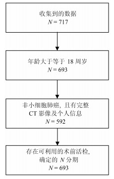
我们收集了广东省人民医院2007年5月至2014年6月期间的717例肺癌病例.这些病人在签署知情同意书后, 自愿提供自己的信息作为研究使用.为了充分利用收集到的数据对非小细胞肺癌淋巴结转移预测, 即对$N1-N3$与$N0$进行有效区分, 我们对收集的数据设置了三个入组标准: 1)年龄大于等于18周岁, 此时的肺部已经发育完全, 消除一定的干扰因素; 2)病理诊断为非小细胞肺癌无其他疾病干扰, 并有完整的CT (Computed tomography)增强图像及个人基本信息; 3)有可利用的术前病理组织活检分级用于确定N分期.经筛选, 共564例病例符合进行肺癌淋巴结转移预测研究的要求(如图 1).
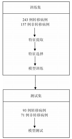
为了得到有价值的结果, 考虑到数据的分配问题, 为了保证客观性, 防止挑数据的现象出现, 在数据分配上, 训练集与测试集将按照时间进行划分, 并以2013年1月为划分点.得到训练集: 400例, 其中, 243例正样本$N1-N3$, 157例负样本$N0$; 测试集: 164例, 其中, 93例正样本, 71例负样本.
1.2 病灶分割
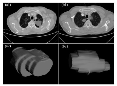
在进行特征提取工作前, 首先要对肿瘤病灶进行分割.医学图像分割的金标准是需要有经验的医生进行手动勾画的结果.但手动分割无法保证每次的分割结果完全一致, 且耗时耗力, 尤其是在数据量很大的情况下.因此, 手动分割不是最理想的做法.在本文中, 使用的自动图像分割算法为基于雪橇的自动区域生长分割算法[11], 该算法首先选定最大切片层的种子点, 这时一般情况下最大切片为中间层的切片, 然后估计肿瘤的大小即直径, 作为一个输入参数, 再自动进行区域生长得到每个切片的肿瘤如图 2(a1), (b1), 之后我们进行雪橇滑动到邻接的上下两个切面, 进行分割, 这样重复上述的区域生长即滑动切片, 最终分割得到多个切片的的肿瘤区域, 我们将肿瘤切面层进行组合, 得到三维肿瘤如图 2(a2), (b2).
1.3 特征的提取与筛选
利用影像组学处理方法, 从分割得到的肿瘤区域中总共提取出386个特征.这些特征可分为四组:三维形状特征, 表面纹理特征, Gabor特征和小波特征[12-13].形状特征通过肿瘤体积、表面积、体积面积比等特征描述肿瘤在空间和平面上的信息.纹理特征通过统计三维不同方向上像素的规律, 通过不同的分布规律来表示肿瘤的异质性. Gabor特征指根据特定方向, 特定尺度筛选出来的纹理信息.
小波特征是指原图像经过小波变换滤波器后的纹理特征.在模式识别范畴中, 高维特征会增加计算复杂度, 此外, 高维的特征往往存在冗余性, 容易造成模型过拟合.因此, 本位通过特征筛选方法首先对所有特征进行降维处理.
本文采用$L$1正则化Lasso进行特征筛选, 对于简单线性回归模型定义为:
$$ \begin{equation} f(x)=\sum\limits_{j=1}^p {w^jx^j} =w^\mathrm{T}x \end{equation} $$ (1) 其中, $x$表示样本, $w$表示要拟合的参数, $p$表示特征的维数.
要进行参数$w$学习, 应用二次损失来表示目标函数, 即:
$$ \begin{equation} J(w)=\frac{1}{n}\sum\limits_{i=1}^n{(y_i-f(x_i)})^2= \frac{1}{n}\vert\vert\ {{y}-Xw\vert\vert}^2 \end{equation} $$ (2) 其中, $X$是数据矩阵, $X=(x_1 , \cdots, x_n)^\mathrm{T}\in {\bf R}^{n\times p}$, ${y}$是由标签组成的列向量, ${y}=(y_1, \cdots, y_n )^\mathrm{T}$.
式(2)的解析解为:
$$ \begin{equation} \hat{w}=(X^\mathrm{T}X)^{-1}X^\mathrm{T}{y} \end{equation} $$ (3) 然而, 若$p\gg n$, 即特征维数远远大于数据个数, 矩阵$X^\mathrm{T}X$将不是满秩的, 此时无解.
通过Lasso正则化, 得到目标函数:
$$ \begin{equation} J_L(w)=\frac{1}{n} \vert\vert{y}-Xw\vert\vert^2+\lambda\vert\vert w\vert\vert _1 \end{equation} $$ (4) 目标函数最小化等价为:
$$ \begin{equation} \mathop {\min }\limits_w \frac{1}{n} \vert\vert{y}-Xw\vert\vert^2, \, \, \, \, \, \, \, \mathrm{s.t.}\, \, \vert \vert w\vert \vert _1 \le C \end{equation} $$ (5) 为了使部分特征排除, 本文采用$L$1正则方法进行压缩.二维情况下, 在$\mbox{(}w^1, w^2)$平面上可画出目标函数的等高线, 取值范围则为平面上半径为$C$的$L$1范数圆, 等高线与$L$1范数圆的交点为最优解. $L$1范数圆和每个坐标轴相交的地方都有"角''出现, 因此在角的位置将产生稀疏性.而在维数更高的情况下, 等高线与L1范数球的交点除角点之外还可能产生在很多边的轮廓线上, 同样也会产生稀疏性.对于式(5), 本位采用近似梯度下降(Proximal gradient descent)[14]算法进行参数$w$的迭代求解, 所构造的最小化函数为$Jl=\{g(w)+R(w)\}$.在每次迭代中, $Jl(w)$的近似计算方法如下:
$$ \begin{align} J_L (w^t+d)&\approx \tilde {J}_{w^t} (d)=g(w^t)+\nabla g(w^t)^\mathrm{T}d\, +\nonumber\\ &\frac{1} {2d^\mathrm{T}(\frac{I }{ \alpha })d}+R(w^t+d)=\nonumber\\ &g(w^t)+\nabla g(w^t)^\mathrm{T}d+\frac{{d^\mathrm{T}d} } {2\alpha } +\nonumber\\ &R(w^t+d) \end{align} $$ (6) 更新迭代$w^{(t+1)}\leftarrow w^t+\mathrm{argmin}_d \tilde {J}_{(w^t)} (d)$, 由于$R(w)$整体不可导, 因而利用子可导引理得:
$$ \begin{align} w^{(t+1)}&=w^t+\mathop {\mathrm{argmin}} \nabla g(w^t)d^\mathrm{T}d\, +\nonumber\\ &\frac{d^\mathrm{T}d}{2\alpha }+\lambda \vert \vert w^t+d\vert \vert _1=\nonumber\\ &\mathrm{argmin}\frac{1 }{ 2}\vert \vert u-(w^t-\alpha \nabla g(w^t))\vert \vert ^2+\nonumber\\ &\lambda \alpha \vert \vert u\vert \vert _1 \end{align} $$ (7) 其中, $S$是软阈值算子, 定义如下:
$$ \begin{equation} S(a, z)=\left\{\begin{array}{ll} a-z, &a>z \\ a+z, &a<-z \\ 0, &a\in [-z, z] \\ \end{array}\right. \end{equation} $$ (8) 整个迭代求解过程为:
输入.数据$X\in {\bf R}^{n\times p}, {y}\in {\bf R}^n$, 初始化$w^{(0)}$.
输出.参数$w^\ast ={\rm argmin}_w\textstyle{1 \over n}\vert \vert Xw-{y}\vert \vert ^2+\\ \lambda \vert\vert w\vert \vert _1 $.
1) 初始化循环次数$t = 0$;
2) 计算梯度$\nabla g=X^\mathrm{T}(Xw-{y})$;
3) 选择一个步长大小$\alpha ^t$;
4) 更新$w\leftarrow S(w-\alpha ^tg, \alpha ^t\lambda )$;
5) 判断是否收敛或者达到最大迭代次数, 未收敛$t\leftarrow t+1$, 并循环2)$\sim$5)步.
通过上述迭代计算, 最终得到最优参数, 而参数大小位于软区间中的, 将被置为零, 即被稀疏掉.
1.4 建立淋巴结转移影像组学标签与预测模型
本文使用LLR对组学特征进行降维并建模, 并使用10折交叉验证, 提高模型的泛化能力, 流程如图 3所示.
将本文使用的影像组学模型的预测概率(Radscore)作为独立的生物标志物, 并与临床指标中显著的特征结合构建多元Logistics模型, 绘制个性化预测的诺模图, 最后通过校正曲线来观察预测模型的偏移情况.
2. 结果
2.1 数据单因素分析结果
我们分别在训练集和验证集上计算各个临床指标与淋巴结转移的单因素P值, 计算方式为卡方检验, 结果见表 1, 发现吸烟与否和EGFR (Epidermal growth factor receptor)基因突变状态与淋巴结转移显著相关.
表 1 训练集和测试集病人的基本情况Table 1 Basic information of patients in the training set and test set基本项 训练集($N=400$) $P$值 测试集($N=164$) $P$值 性别 男 144 (36 %) 0.896 78 (47.6 %) 0.585 女 256 (64 %) 86 (52.4 %) 吸烟 是 126 (31.5 %) 0.030* 45 (27.4 %) 0.081 否 274 (68.5 %) 119 (72.6 %) EGFR 缺失 36 (9 %) 4 (2.4 %) 突变 138 (34.5 %) $ < $0.001* 67 (40.9 %) 0.112 正常 226 (56.5 %) 93 (56.7 %) 2.2 淋巴结转移影像组学标签
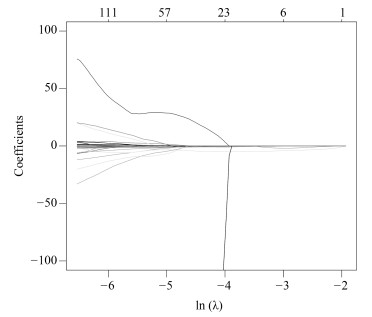
影像组学得分是每个病人最后通过模型预测后的输出值, 随着特征数的动态变化, 模型输出的AUC (Area under curve)值也随之变化, 如图 4所示, 使用R语言的Glmnet库可获得模型的参数$\lambda $的变化图.图中直观显示了参数$\lambda $的变化对模型性能的影响, 这次实验中模型选择了3个变量.如图 5所示, 横坐标表示$\lambda $的变化, 纵坐标表示变量的系数变化, 当$\lambda $逐渐变大时, 变量的系数逐渐减少为零, 表示变量选择的过程, 当$\lambda $越大表示模型的压缩程度越大.
 图 4 $\lambda $与变量数目对应走势Fig. 4 The trend of the parameters and the number of variables
通过套索回归方法, 自动的将变量压缩为3个, 其性能从图 4中也可发现, 模型的AUC值为最佳, 最终的特征如表 2所示. $V0$为截距项; $V179$为横向小波分解90度共生矩阵Contrast特征; $V230$为横向小波分解90度共生矩阵Entropy特征.
表 2 Lasso选择得到的参数Table 2 Parameters selected by LassoLasso选择的参数 含义 数值 $P$值 $V0$ 截距项 2.079115 $V179$ 横向小波分解90度共生矩阵Contrast特征(Contrast_2_90) 0.0000087 < 0.001*** $V230$ 横向小波分解90度共生矩阵Entropy特征(Entropy_3_180) $-$3.573315 < 0.001*** $V591$ 表面积与体积的比例(Surface to volume ratio) $-$1.411426 < 0.001*** $V591$为表面积与体积的比例; 将三个组学特征与$N$分期进行单因素分析, 其$P$值都是小于0.05, 表示与淋巴结转移有显著相关性.根据Lasso选择后的三个变量建立Logistics模型并计算出Rad-score, 详见式(9).并且同时建立SVM (Support vector machine)模型.
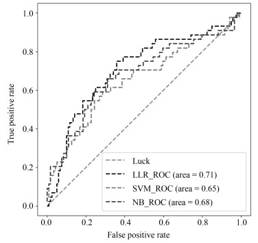
NB (Naive Bayesian)模型, 进行训练与预测, LLR模型训练集AUC为0.710, 测试集为0.712, 表现较优; 如表 3所示.将实验中使用的三个机器学习模型的结果进行对比, 可以发现, LLR的实验结果是最好的.
表 3 不同方法对比结果Table 3 Comparison results of different methods方法 训练集(AUC) 测试集(AUC) 召回率 LLR 0.710 0.712 0.75 SVM 0.698 0.654 0.75 NB 0.718 0.681 0.74 $$ \begin{equation} \begin{aligned} &\text{Rad-score}=2.328373+{\rm Contrast}\_2\_90\times\\ &\qquad 0.0000106 -{\rm entropy}\_3\_180\times 3.838207 +\\ &\qquad\text{Maximum 3D diameter}\times 0.0000002 -\\ &\qquad\text{Surface to volume ratio}\times 1.897416 \\ \end{aligned} \end{equation} $$ (9) 2.3 诺模图个性化预测模型
为了体现诺模图的临床意义, 融合Rad-score, 吸烟情况和EGFR基因因素等有意义的变量进行分析, 绘制出个性化预测的诺模图, 如图 7所示.为了给每个病人在最后得到一个得分, 需要将其对应变量的得分进行相加, 然后在概率线找到对应得分的概率, 从而实现非小细胞肺癌淋巴结转移的个性化预测.我们通过一致性指数(Concordance index, $C$-index)对模型进行了衡量, 其对应的$C$-index为0.724.
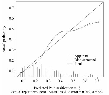
本文中使用校正曲线来验证诺模图的预测效果, 如图 8所示, 由校正曲线可以看出, 预测结果基本上没有偏离真实标签的结果, 表现良好, 因此, 该模型具有可靠的预测性能[15].
3. 结论
在构建非小细胞肺癌淋巴结转移的预测模型中, 使用LLR筛选组学特征并构建组学标签, 并与显著的临床特征构建多元Logistics模型, 绘制个性化预测的诺模图.其中LLR模型在训练集上的AUC值为0.710, 在测试集上的AUC值为0.712, 利用多元Logistics模型绘制个性化预测的诺模图, 得到模型表现能力$C$-index为0.724 (95 % CI: 0.678 $\sim$ 0.770), 并且在校正曲线上表现良好, 所以个性化预测的诺模图在临床决策上可起重要参考意义.[16].
-
[1] 段广仁.高阶全驱系统方法—Ⅱ.能控性与全驱性.自动化学报, 2020, 46(8): 1571-1581 doi: 10.16383/j.aas.c200369Duan Guang-Ren. High-order system approaches: Ⅱ. Controllability and fully-actuation. Acta Automatica Sinica, 2020, 46(8): 1571-1581 doi: 10.16383/j.aas.c200369 [2] Tsinias J, Kitsos C. Observability and state estimation for a class of nonlinear systems. IEEE Transactions on Automatic Control, 2019, 64(6): 2621-2628 doi: 10.1109/TAC.2018.2868458 [3] Bartosiewicz Z. Local observability of nonlinear positive continuous-time systems. Automatica, 2017, 78: 135-138 doi: 10.1016/j.automatica.2016.12.037 [4] 陈彭年, 韩正之, 张钟俊.仿射非线性系统的动态输出反馈镇定.自动化学报, 1997, 23(3): 338-344 http://www.aas.net.cn/article/id/17038Chen Peng-Nian, Han Zheng-Zhi, Zhang Zhong-Jun. Dynamic output feedback stabilization of affine nonlinear systems. Acta Automatica Sinica, 1997, 23(3): 338-344 http://www.aas.net.cn/article/id/17038 [5] 韩志涛, 段晓东, 张嗣瀛.非线性大系统的弱能观性.东北大学学报(自然科学版), 2003, 24(12): 1123-1125 http://www.wanfangdata.com.cn/details/detail.do?_type=perio&id=dbdxxb200312001Han Zhi-Tao, Duan Xiao-Dong, Zhang Si-Ying. Weak observability of nonlinear large-scale system. Journal of Northeastern University (Natural Science), 2003, 24(12): 1123-1125 http://www.wanfangdata.com.cn/details/detail.do?_type=perio&id=dbdxxb200312001 [6] Martinelli A. Nonlinear unknown input observability: Extension of the observability rank condition. IEEE Transactions on Automatic Control, 2019, 64(1): 222-237 http://ieeexplore.ieee.org/document/8270358/ [7] 韩正之, 潘丹杰, 张钟俊.非线性系统的能观性和状态观测器.控制理论与应用, 1990, 7(4): 1-9 http://www.cqvip.com/QK/91549X/19903/314118.htmlHan Zheng-Zhi, Pan Dan-Jie, Zhang Zhong-Jun. Observability and observers of nonlinear systems. Control Theory & Applications, 1990, 7(4): 1-9 http://www.cqvip.com/QK/91549X/19903/314118.html [8] 程代展, 秦化淑.非线性系统的几何方法(下)—目前动态与展望.控制理论与应用, 1987, 4(2): 1-9 http://www.cnki.com.cn/Article/CJFDTotal-KZLY198702000.htmCheng Dai-Zhan, Qin Hua-Shu. Geometric methods for nonlinear systems (Part 2): Current dynamics and prospects. Control Theory & Applications, 1987, 4(2): 1-9 http://www.cnki.com.cn/Article/CJFDTotal-KZLY198702000.htm [9] Terrell W J. Local observability of nonlinear differential-algebraic equations (DAEs) from the linearization along a trajectory. IEEE Transactions on Automatic Control, 2001, 46(12): 1947-1950 doi: 10.1109/9.975497 [10] Hespanha J P, Liberzon D, Angeli D, Sontag E D. Nonlinear norm-observability notions and stability of switched systems. IEEE Transactions on Automatic Control, 2005, 50(2): 154-168 http://www.wanfangdata.com.cn/details/detail.do?_type=perio&id=814cc96835395d60e85f49c36f590632 [11] Cai S T, Xiao M Q. Boundary observability of wave equations with nonlinear van der pol type boundary conditions. Automatica, 2018, 98: 350-353 doi: 10.1016/j.automatica.2018.09.008 [12] 程代展, 王洪才.一般非线性系统的Kalman分解.自动化学报, 1989, 15(1): 30-36 http://www.aas.net.cn/article/id/14936Cheng Dai-Zhan, Wang Hong-Cai. Kalman decomposition of general nonlinear systems. Acta Automatica Sinica, 1989, 15(1): 30-36 http://www.aas.net.cn/article/id/14936 [13] Lin W, Byrnes C I. Zero-state observability and stability of discrete-time nonlinear systems. Automatica, 1995, 31(2): 269-274 doi: 10.1016/0005-1098(94)00088-Z [14] Hanba S. Further results on the uniform observability of discrete-time nonlinear systems. IEEE Transactions on Automatic Control, 2010, 55(4): 1034-1038 doi: 10.1109/TAC.2010.2041983 [15] Anguelova M, Wennberg B. On analytic and algebraic observability of nonlinear delay systems. Automatica, 2010, 46(4): 682-686 doi: 10.1016/j.automatica.2010.01.031 [16] Chen Z Y. On observability of nonlinear steady-state generators. Automatica, 2010, 46(10): 1712-1718 doi: 10.1016/j.automatica.2010.06.028 [17] 张敏, 罗安, 沈洪远, 王京.一类非线性系统观测器与算例.控制理论与应用, 2002, 19(4): 541-544 http://www.wanfangdata.com.cn/details/detail.do?_type=perio&id=kzllyyy200204011Zhang Min, Luo An, Shen Hong-Yuan, Wang Jing. Observer for a class of nonlinear system and an example. Control Theory & Applications, 2002, 19(4): 541-544 http://www.wanfangdata.com.cn/details/detail.do?_type=perio&id=kzllyyy200204011 [18] Shim H, Seo J H. Recursive nonlinear observer design: Beyond the uniform observability. IEEE Transactions on Automatic Control, 2003, 48(2): 294-298 doi: 10.1109/TAC.2002.808485 [19] 韩正之, 郑毓蕃, 张钟俊.非线性系统的一种新标准型(Ⅰ)—观察器型.数学物理学报, 1992, 12(3): 318-324 http://www.cnki.com.cn/Article/CJFDTotal-SXWX199203010.htmHan Zheng-Zhi, Zheng Yu-Fan, Zhang Zhong-Jun. A new standard type of nonlinear system (Ⅰ). Observers. Acta Mathematica Scientia, 1992, 12(3): 318-324 http://www.cnki.com.cn/Article/CJFDTotal-SXWX199203010.htm [20] Astolfi D, Possieri C. Design of local observers for autonomous nonlinear systems not in observability canonical form. Automatica, 2019, 103: 443-449 doi: 10.1016/j.automatica.2019.02.030 [21] Hanba S. On the "uniform" observability of discrete-time nonlinear systems. IEEE Transactions on Automatic Control, 2009, 54(8): 1925-1928 doi: 10.1109/TAC.2009.2023775 [22] 段广仁.飞行器控制的伪线性系统方法—第一部分:综述与问题.宇航学报, 2020, 41(6): 633-646 http://www.cqvip.com/QK/95668X/202006/7102487436.htmlDuan Guang-Ren. Quasi-linear system approaches for flight vehicle control—Part 1: An overview and problems. Journal of Astronautics, 2020, 41(6): 633-646 http://www.cqvip.com/QK/95668X/202006/7102487436.html [23] 段广仁.飞行器控制的伪线性系统方法—第二部分:方法与展望.宇航学报, 2020, 41(7): 839-849 http://www.cqvip.com/QK/95668X/202006/7102487436.htmlDuan Guang-Ren. Quasi-linear system approaches for flight vehicle control—Part 2: Methods and prospects. Journal of Astronautics, 2020, 41(7): 839-849 http://www.cqvip.com/QK/95668X/202006/7102487436.html [24] Kalman R. On the general theory of control systems. IRE Transactions on Automatic Control, 1959, 4(3): 110 doi: 10.1109/TAC.1959.1104873 [25] 高为炳, 程勉, 夏小华.非线性控制系统的发展.自动化学报, 1991, 17(5): 513-524 http://www.aas.net.cn/article/id/14560Gao Wei-Bing, Cheng Mian, Xia Xiao-Hua. The development of nonlinear control systems. Acta Automatica Sinica, 1991, 17(5): 513-524 http://www.aas.net.cn/article/id/14560 [26] Casti J L. Recent developments and future perspectives in nonlinear system theory. SIAM Review, 1982, 24(3): 301-331 doi: 10.1137/1024065 [27] Brocket R W. Asymptotic stability and feedback stabilization. Differential Geometric Control Theory. Boston: Birkhauser, 1983. 112-121 [28] 韩正之, 刘建华, 郑毅, 张钟俊.非线性控制系统的特性(Ⅰ).控制与决策, 1994, 9(4): 315-320 http://www.cnki.com.cn/Article/CJFDTotal-KZYC404.015.htmHan Zheng-Zhi, Liu Jian-Hua, Zheng Yi, Zhang Zhong-Jun. Characters of nonlinear control systems (Ⅰ). Control and Decision, 1994, 9(4): 315-320 http://www.cnki.com.cn/Article/CJFDTotal-KZYC404.015.htm [29] 李文林, 高为炳.非线性控制系统的可控标准型问题.航空学报, 1989, 10(5): 249-258 http://www.cnki.com.cn/Article/CJFDTotal-HKXB198905006.htmLi Wen-Lin, Gao Wei-Bing. Controllability canonical form for nonlinear control systems. Acta Aeronautica ET Astronautica Sinica, 1989, 10(5): 249-258 http://www.cnki.com.cn/Article/CJFDTotal-HKXB198905006.htm [30] 段广仁.线性系统理论(上下册).第3版.北京:科学出版社, 2016.Duan Guang-Ren. Linear System Theory(two volumes) (Third edition). Beijing: Science Press, 2016. [31] Duan G R, Gao Y J. State-space realization and generalized Popov Belevitch Hautus criterion for high-order linear systems—The singular case. International Journal of Control, Automation and Systems, 2020, 18(8): 2038-2047 doi: 10.1007/s12555-019-0212-4 [32] Duan G R. Analysis and Design of Descriptor Linear Systems. New York, USA: Springer, 2010. [33] Duan G R. Solution to matrix equation AV + BW = EVF and eigenstructure assignment for descriptor systems. Automatica, 1992, 28(3): 639-643 doi: 10.1016/0005-1098(92)90191-H [34] Duan G R, Patton R J. Eigenstructure assignment in descriptor systems via state feedback—A new complete parametric approach. International Journal of Systems Science, 1998, 29(2): 167-178 http://www.wanfangdata.com.cn/details/detail.do?_type=perio&id=10.1080/00207729808929509 [35] Duan G R. Eigenstructure assignment and response analysis in descriptor linear systems with state feedback control. International Journal of Control, 1998, 69(5): 663-694 doi: 10.1080/002071798222622 [36] Duan G R. Parametric eigenstructure assignment in second-order descriptor linear systems. IEEE Transactions on Automatic Control, 2004, 49(10): 1789-1795 doi: 10.1109/TAC.2004.835580 [37] 段广仁.高阶系统方法—Ⅰ.全驱系统与参数化设计.自动化学报, 2020, 46(7): 1333-1345 doi: 10.16383/j.aas.c200234Duan Guang-Ren. High-order system approaches: Ⅰ. Fully-actuated systems and parametric design. Acta Automatica Sinica, 2020, 46(7): 1333-1345 doi: 10.16383/j.aas.c200234 期刊类型引用(14)
1. 王圣洁,刘乾义,文超,李忠灿,田文华. 考虑致因的初始晚点影响列车数预测模型研究. 综合运输. 2024(02): 105-110 .  百度学术
百度学术2. 刘鲁岳,肖宝弟,岳丽丽. 基于改进RF-XGBoost算法的列车运行晚点预测研究. 铁道标准设计. 2023(03): 38-43 . 百度学术3. 李建民,许心越,丁忻. 基于多阶段特征优选的高速铁路列车晚点预测模型. 中国铁道科学. 2023(04): 219-229 . 百度学术4. 林鹏,田宇,袁志明,张琦,董海荣,宋海锋,阳春华. 高速铁路信号系统运维分层架构模型研究. 自动化学报. 2022(01): 152-161 . 本站查看5. 文超,李津,李忠灿,智利军,田锐,宋邵杰. 机器学习在铁路列车调度调整中的应用综述. 交通运输工程与信息学报. 2022(01): 1-14 . 百度学术6. 张芸鹏,朱志强,王子维. 高速铁路行车调度作业风险管控信息系统设计研究. 铁道运输与经济. 2022(03): 47-52+59 . 百度学术7. 张红斌,李军,陈亚茹. 京沪高铁列车运行晚点预测方法研究. 铁路计算机应用. 2022(05): 1-6 . 百度学术8. 俞胜平,韩忻辰,袁志明,崔东亮. 基于策略梯度强化学习的高铁列车动态调度方法. 控制与决策. 2022(09): 2407-2417 . 百度学术9. 唐涛,甘婧. 基于国内外铁路运营数据的列车运行时间预测模型. 中国安全科学学报. 2022(06): 123-130 . 百度学术10. 刘睿,徐传玲,文超. 基于马尔科夫链的高铁列车连带晚点横向传播. 铁道科学与工程学报. 2022(10): 2804-2812 . 百度学术11. 廖璐,张亚东,葛晓程,郭进,禹倩. 基于GBDT的列车晚点时长预测模型研究. 铁道标准设计. 2021(08): 149-154+176 . 百度学术12. 闫璐,张琦,王荣笙,丁舒忻. 基于动力学特性的列车运行态势分析. 铁道运输与经济. 2021(08): 64-70 . 百度学术13. 张俊,张欣愉,叶玉玲. 高速铁路非正常事件下初始延误场景聚类研究. 物流科技. 2021(06): 1-4+9 . 百度学术14. 徐传玲,文超,胡瑞,冯永泰. 高速铁路列车连带晚点产生机理及其判定. 交通运输工程与信息学报. 2020(04): 31-37 . 百度学术其他类型引用(28)
-

 下载:
下载:

计量
- 文章访问数: 2087
- HTML全文浏览量: 506
- PDF下载量: 721
- 被引次数: 42
 下载:
下载:
