

Customized Interior-point Method for Cooperative Trajectory Planning of Multiple Unmanned Aerial Vehicles
-
摘要: 为提高多无人机(Unmanned aerial vehicles, UAV)协同轨迹规划(Cooperative trajectory planning, CTP)效率, 在解耦序列凸优化(Sequential convex programming, SCP)方法基础上, 提出一种高效求解凸优化子问题的定制内点法. 首先引入松弛变量, 构建子问题的等价描述形式, 并推导该形式下的子问题最优性条件. 然后在预测−校正原对偶内点法的框架下, 构建一套高效求解最优性条件方程组的计算流程以降低子问题计算复杂度, 并利用约束矩阵特征提出一种快速计算原对偶搜索方向的方法以提高规划效率. 仿真结果表明, 在解耦序列凸优化框架下, 定制内点法可将协同轨迹规划耗时降低一个数量级, 达到秒级.Abstract: To improve the efficiency of cooperative trajectory planning (CTP) for multiple unmanned aerial vehicles (UAVs), a customized interior-point method is proposed for efficiently solving convex subproblems within the decoupled sequential convex programming (SCP) method. Firstly, slack variables are introduced to construct an equivalent form of the subproblem, and the optimality conditions of the subproblem in this equivalent form are derived. Then, under the frame of the predictor-corrector primal-dual interior-point method, an efficient computation procedure for solving the equations of optimality conditions is developed. And through exploring the matrix characteristics of constraints to reduce the complexity of solving subproblems, a fast generation method for primal-dual search direction is proposed to improve the planning efficiency. Simulation results demonstrate that the customized interior-point method can decrease the computation times of CTP by one order of magnitude to several seconds.
-
多无人机(Unmanned aerial vehicle, UAV)协同通过功能互补和能力叠加等方式可以提高任务完成效能, 已成为无人机应用的重要发展趋势[1], 协同轨迹规划(Cooperative trajectory planning, CTP)则是系统关键技术之一.
针对轨迹规划存在的非线性、约束多、变量维度高等计算复杂难题, 近年来序列凸优化(Sequential convex programming, SCP)方法受到广泛关注[2]. SCP利用凸优化算法具有迭代计算上界和多项式时间复杂度[3]的特点, 通过求解一系列凸优化子问题[4], 可快速获得原非凸问题的局部最优解, 其优势已在不同轨迹规划领域得到验证. 相比基于采样的轨迹规划方法, SCP具有更强的高维求解能力且无需进行光滑处理[5-6]; 相比伪谱法, SCP能够在不降低优化性能的条件下极大地提高求解效率[7-8]; 相比启发式算法, SCP具有更好的寻优和收敛能力[9-10].
在协同轨迹规划研究方面, 文献[11]首次将SCP应用于四旋翼飞行器协同轨迹规划; 文献[12]进一步提出增量SCP以提高算法收敛速度; Morgan等[13]提出分散SCP以快速生成集群重构轨迹, 并基于四旋翼完成了实验验证; 针对固定翼无人机, 文献[14]提出一种罚函数SCP方法实现了多机协同轨迹规划; 文献[15]提出一种解耦SCP方法, 通过并行求解降低了算法耗时随无人机数量的增长程度.
虽然SCP相比于传统轨迹规划方法具有效率优势, 但固定翼无人机编队轨迹规划仍需数十秒[14-16], 难以满足动态规划需求. 对此, 本文在SCP基础上, 从子问题求解性能角度开展研究, 通过定制凸优化算法降低子问题优化耗时, 从而提高规划效率.
凸优化子问题一般采用SeDuMi[17]和Mosek[18]等工具包求解, 但工具包为保证稳定性需增加额外运算成本, 同时难以针对具体问题设计高效求解过程. 已有的内点法定制研究表明, 通过算法定制能够显著提高凸优化效率. Dueri等[19]对火箭回收轨迹规划进行内点法定制, 实现了轨迹实时规划, 并完成了实验验证. Xu等[20]通过定制稀疏内点法, 将单个四旋翼轨迹规划耗时控制在1 s以内. 但是, 定制算法不具有广泛通用性, 例如针对火箭或四旋翼轨迹规划的定制内点法无法直接应用于固定翼无人机. 根据文献调研, 尚无针对单架或多架固定翼无人机轨迹规划的定制凸优化算法.
固定翼无人机的动力学呈非线性, 同时多无人机系统还需考虑机间协同约束, 这些因素都增加了轨迹规划复杂度. 对此, 本文在解耦SCP[15]的架构下, 研究子问题求解的定制内点法, 通过减少单次凸优化耗时, 进一步提升多无人机协同轨迹规划效率.
1. 问题建模
多无人机协同轨迹规划需要根据每架无人机的起始点和目标点, 考虑运动方程、终端条件、边界条件、避障和避碰等约束, 以最小化时间或能量等为性能指标, 为所有无人机生成可行的飞行轨迹.
本文以时间最短为目标, 将无人机协同轨迹规划建模为下述最优控制问题P1[15]:
$$\begin{split} {\rm{P}}1\;:&\mathop {\min }\limits_{{{\boldsymbol{s}}_i}(t),{{\boldsymbol{u}}_i}(t),{t_f},i = 1,2, \cdots ,N} \;\;\;{t_f} \\ &{\rm{s}}{\rm{. t}}{\rm{.}}\;\;\forall i = 1,2, \cdots ,N \\ &\{{{{\boldsymbol{\dot s}}}_i} = f({{\boldsymbol{s}}_i},{{\boldsymbol{u}}_i},t) \\ &{{\boldsymbol{s}}_i}({t_0}) = {{\boldsymbol{s}}_{i,0}}\; \\ &{{\boldsymbol{s}}_i}({t_f}) = {{\boldsymbol{s}}_{i,f}} \\ &{{\boldsymbol{s}}_{\min }} \leq {{\boldsymbol{s}}_i}(t) \leq {{\boldsymbol{s}}_{{\rm{max}}}} \\ &{{\boldsymbol{u}}_{\min }} \leq {{\boldsymbol{u}}_i}(t) \leq {{\boldsymbol{u}}_{\max }} \\ &||{\boldsymbol{C}} \cdot [{{\boldsymbol{s}}_i}(t) - {{\boldsymbol{p}}_{{\rm{obs}},m}}]|{|_2} \geq {r_m},\;\forall m = 1,2, \cdots ,M \\ &||{\boldsymbol{C}} \cdot [{{\boldsymbol{s}}_i}(t) - {{\boldsymbol{s}}_j}(t)]|{|_2} \geq R,\;\;\forall j = 1,2, \cdots ,N \\ &i \ne j \} \\[-11pt] \end{split} $$ (1) 其中, 下标i表示无人机编号; 下标0表示变量初始时刻值; 下标f表示变量终端时刻值; N为无人机数量; t为飞行时间; ${\boldsymbol{s}}_i $表示无人机i的状态量且${{\boldsymbol{s}}_i} = {({x_i},{y_i},{h_i},{v_i},{\chi _i},{\gamma _i})^{\rm{T}}}$; smax和smin为状态量上下限; ${\boldsymbol{u}}_i $表示无人机i的控制量且${{\boldsymbol{u}}_i} = {\rm{ (}}{n_{x,i}},{n_{y,i}}, {n_{z,i}}{{\rm{)}}^{\rm{T}}}$; umax和umin为控制量上下限; pobs,m和rm为障碍m的位置和半径; M表示障碍数量; C = [I2×2, 04×4]; R为机间避碰安全距离.
图1给出了多无人机协同轨迹规划问题及部分参数的示意图.
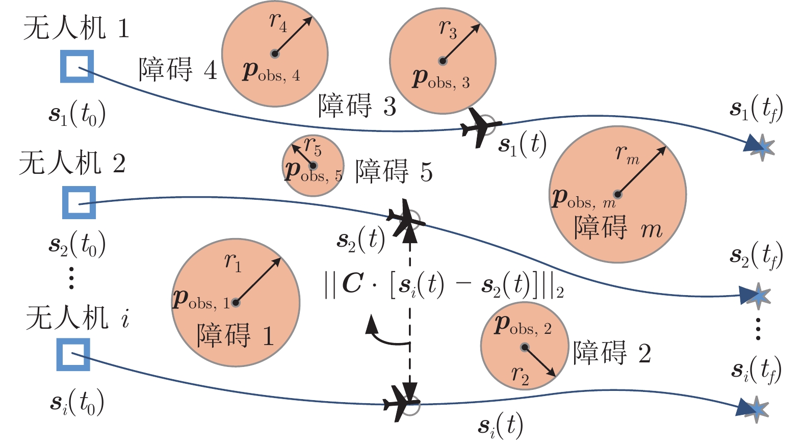 图 1 多无人机协同轨迹规划问题示意图Fig. 1 Illustration of multi-UAV cooperative trajectory planning problems
问题P1中各子式的意义可参见文献[15-16]. 其中, 运动方程${{\boldsymbol{\dot s}}_i} = f({{\boldsymbol{s}}_i},{{\boldsymbol{u}}_i},t)$的表达式[15]如式(2)所示. 其中, (x, y)为水平位置; h为高度; v为速度; $\chi $为航向角; $\gamma $为航迹倾角; g为重力加速度值; nx, ny, nz分别为无人机在切向、水平、铅垂方向的过载.
$$\left\{ \begin{aligned} &{{\dot x}_i} = {v_i}\cos {\gamma _i}\cos {\chi _i} \\ &{{\dot y}_i} = {v_i}\cos {\gamma _i}\sin {\chi _i} \\ & {{\dot h}_i} = {v_i}\sin {\gamma _i} \\ &{{\dot v}_i} = g \cdot ({n_{x,i}} - \sin {\gamma _i}) \\ & {{\dot \chi }_i} = {\frac{g \cdot {n_{y,i}}}{{v_i}\cos {\gamma _i}}} \\ &{{\dot \gamma }_i} = {g \cdot \frac{{n_{z,i}} - \cos {\gamma _i}}{{v_i}}} \end{aligned} \right.$$ (2) 2. 解耦SCP方法
针对式(1)所述的最优控制问题, 文献[15]给出了一种解耦SCP求解架构. 本文在该架构的基础上, 聚焦凸优化子问题的定制内点法研究. 考虑文章完整性, 本节对解耦SCP方法进行简述.
基于SCP的无人机轨迹规划步骤可概括为: 1)采用配点法将最优控制问题转化为非凸优化问题; 2)利用约束凸化构建一系列凸优化子问题; 3)通过迭代求解凸优化子问题, 获得非凸优化问题的解, 即最优控制问题的数值近似解.
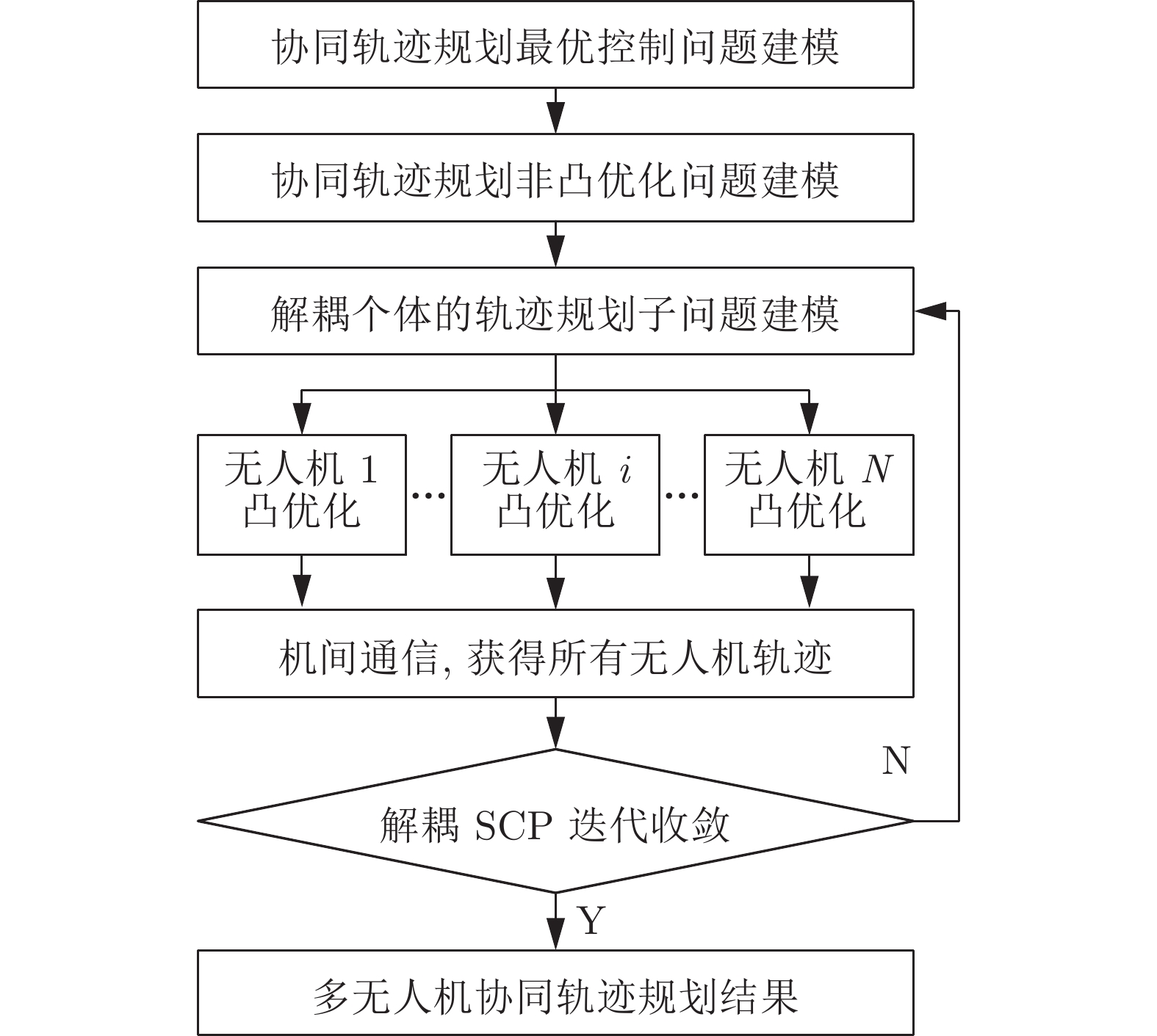
在SCP基础上, 解耦SCP进一步针对协同规划问题, 利用轨迹冻结思想和协调约束机制, 将关于多机轨迹的一个优化问题解耦为一组优化问题, 解耦后每个问题的优化变量仅为一架无人机的轨迹, 且解耦问题支持并行求解, 提高了协同轨迹规划效率. 解耦SCP方法的求解架构如图2所示.
针对式(1)所述的问题P1, 利用梯形积分和约束凸化, 并引入罚函数和信赖域, 可构建解耦SCP方法中需多无人机并行迭代求解的凸优化子问题P2[15], 如式(3)所示.
$$\begin{split} {\rm{P}}2:\; &\mathop {\min }\limits_{{{\boldsymbol{z}}_i}} \;\;\Delta {t_i}\;\; + \;\;\mu \cdot \sum\limits_{l = 1}^{{n_{{\rm{eq}}}}} {|{h_l}({{\boldsymbol{z}}_i})|} \;+ \\ & \qquad\mu \cdot \sum\limits_{l = 1}^{{n_{{\rm{in}}}}} {\max \left( {{g_l}({{\boldsymbol{z}}_i}),0} \right)} \\ &{\rm{s}}{\rm{. t}}{\rm{.}}\;\left| {{{\boldsymbol{s}}_i}[k] - {{{\boldsymbol{\bar s}}}_i}[k]} \right| \leq {\boldsymbol{\rho }},\;k = 1,\cdots,K \end{split} $$ (3) 其中, ${{\boldsymbol{z}}_i} \in {{\bf{R}}^{{n_z} \times 1}}$为无人机i的轨迹优化变量, 如式(4)所示, $n_z $表示优化变量维度; $\Delta t $为离散时间步长; μ为罚系数; neq和nin分别为等式和不等式约束的数量; ${h_l},\;l = 1,2,\cdots,{n_{{\rm{eq}}}}$表示离散的等式凸约束, 即式(5) ~ (7), 其中, $\tilde {\boldsymbol{A}}$, $\tilde {\boldsymbol{B}}$, $\tilde {\boldsymbol{C}}$, $\tilde{\boldsymbol{ D}}$为运动方程线性化后的系数矩阵, 具体表达式见文献[15]; ${g_l},\;l = 1,2,\cdots,{n_{{\rm{in}}}}$表示离散的不等式凸约束, 即式(8) ~ (12), 其中, $\overline {\Delta t} $为凸化时的基准步长, ${\Pi _i}$为无人机i需规避的其他无人机集合; ${\boldsymbol{\rho }}$为信赖域半径; k为离散时刻; K为离散区间数量; ${\boldsymbol{\bar s}}$为约束凸化时的基准状态.
$${{\boldsymbol{z}}_i} = {({\boldsymbol{s}}_i^{\rm{T}}[0],\cdots,{\boldsymbol{s}}_i^{\rm{T}}[K],{\boldsymbol{u}}_i^{\rm{T}}[0],\cdots,{\boldsymbol{u}}_i^{\rm{T}}[K],\Delta {t_i})^{\rm{T}}}$$ (4) $$\begin{split} {{\tilde {\boldsymbol{A}}}_{k{\rm{ + 1}}}} \cdot &{{\boldsymbol{s}}_i}[k + 1] + {{\tilde {\boldsymbol{A}}}_k} \cdot {{\boldsymbol{s}}_i}[k] + {{\tilde {\boldsymbol{B}}}_{k{\rm{ + 1}}}} \cdot {{\boldsymbol{u}}_i}[k + 1] \;+ \\ &{{\tilde {\boldsymbol{B}}}_k} \cdot {{\boldsymbol{u}}_i}[k] + ({{\tilde {\boldsymbol{C}}}_k} + {{\tilde {\boldsymbol{C}}}_{k + 1}})\Delta t + {{\tilde {\boldsymbol{D}}}_k}\; + \\ & {{\tilde {\boldsymbol{D}}}_{k + 1}} = 0,\;\;\;k = 0,1,\cdots,K - 1 \end{split}$$ (5) $${{\boldsymbol{s}}_i}[0] = {{\boldsymbol{s}}_{i,0}}$$ (6) $${{\boldsymbol{s}}_i}[K] = {{\boldsymbol{s}}_{i,f}}$$ (7) $${{\boldsymbol{s}}_{\min }} \leq {{\boldsymbol{s}}_i}[k] \leq {{\boldsymbol{s}}_{{\rm{max}}}},\;k = 0,1, \cdots ,K$$ (8) $${{\boldsymbol{u}}_{\min }} \leq {{\boldsymbol{u}}_i}[k] \leq {{\boldsymbol{u}}_{\max }},\;k = 0,1, \cdots ,K$$ (9) $$\Delta {t_i} \geq \mathop {\max }\limits_{i \in \{ 1,2,\cdots,N\} } \left( {{{\overline {\Delta t} }_i}} \right)$$ (10) $$\begin{split} &\dfrac{{{{({\boldsymbol{C}} \cdot {{{\boldsymbol{\bar s}}}_i}[k] - {{\boldsymbol{p}}_{{\rm{obs}},m}})}^{\rm{T}}}{\boldsymbol{C}}({{\boldsymbol{s}}_i}[k] - {{{\boldsymbol{\bar s}}}_i}[k])\;\;\;\;}}{{||{\boldsymbol{C}} \cdot {{{\boldsymbol{\bar s}}}_i}[k] - {{\boldsymbol{p}}_{{\rm{obs}},m}}||}} \geq \\ &\qquad{r_m} - ||{\boldsymbol{C}} \cdot {{{\boldsymbol{\bar s}}}_i}[k] - {{\boldsymbol{p}}_{{\rm{obs}},m}}|| \end{split} $$ (11) $$\begin{split} & \dfrac{{{{({\boldsymbol{C}}({{{\boldsymbol{\bar s}}}_i}[k] - {{{\boldsymbol{\bar s}}}_j}[k]))}^{\rm{T}}} \cdot \left( {{\boldsymbol{C}}({{\boldsymbol{s}}_i}[k] - {{{\boldsymbol{\bar s}}}_i}[k])} \right)}}{{||{\boldsymbol{C}}({{{\boldsymbol{\bar s}}}_i}[k] - {{{\boldsymbol{\bar s}}}_j}[k])||}}\; \geq \\ &\qquad {{R}} - ||{\boldsymbol{C}}({{{\boldsymbol{\bar s}}}_i}[k] - {{{\boldsymbol{\bar s}}}_j}[k])||\;,\;\;\;\;j \in {\Pi _i} \end{split}$$ (12) 3. 子问题最优性条件
为了开展内点法定制研究, 本节首先构建子问题的一种等价描述形式, 然后基于最优化理论构建该形式下的结果最优性条件.
3.1 凸优化子问题的等价描述形式
为了方便表述和推导, 将问题P2罚函数中的所有等式约束统一表示为式(13), 包括运动约束式(5)以及终端约束式(6)和式(7), 其中zi简记为z.
$${{{\boldsymbol{A}}_{{\rm{eq}}}}} \cdot {\boldsymbol{z}} = {{\boldsymbol{b}}_{{\rm{eq}}}}$$ (13) 其中, ${{{\boldsymbol{A}}_{{\rm{eq}}}}} \in {{\bf{R}}^{{n_{{\rm{eq}}}} \times {n_z}}}$和${{\boldsymbol{b}}_{{\rm{eq}}}} \in {{\bf{R}}^{{n_{{\rm{eq}}}} \times 1}}$表示等式约束的系数矩阵和右端项, 可根据式(5) ~ (7)获得.
将不等式约束统一表示为式(14), 包括边界约束式(8) ~ (10)、避障约束式(11)和避碰约束式(12), 即
$${{\boldsymbol{A}}_{{\rm{in}}}} \cdot {\boldsymbol{z}} \leq {{\boldsymbol{b}}_{{\rm{in}}}}$$ (14) 其中, ${{\boldsymbol{A}}_{{\rm{in}}}} \in {{\bf{R}}^{{n_{{\rm{in}}}} \times {n_z}}}$和${{\boldsymbol{b}}_{{\rm{in}}}} \in {{\bf{R}}^{{n_{{\rm{in}}}} \times 1}}$表示不等式约束的系数矩阵和右端项向量, 可根据式(8) ~ (12)获得.
将信赖域表示为式(15), 其中${{\boldsymbol{A}}_{{\rm{tr}}}} \in {{\bf{R}}^{{n_{{\rm{tr}}}} \times {n_z}}}$和${{\boldsymbol{b}}_{{\rm{tr}}}} \in {{\bf{R}}^{{n_{{\rm{tr}}}} \times 1}}$表示信赖域约束的系数矩阵和右端项向量, $n_{\rm{tr}}$为信赖域约束数量.
$${{\boldsymbol{A}}_{{\rm{tr}}}} \cdot {\boldsymbol{z}} \leq {{\boldsymbol{b}}_{{\rm{tr}}}}$$ (15) 由于凸优化子问题P2的约束式(6) ~ (12)均具有线性特征, 因此上述表述是可行的. 在此约束表示形式下, 凸优化子问题P2可表示为子问题P3
$$ \begin{split} {\rm{P}}3:\;&\mathop {\min }\limits_{\boldsymbol{z}} \;\;{{\boldsymbol{q}}^{\rm{T}}} \cdot {\boldsymbol{z}} + \mu \cdot \sum\limits_{l = 1}^{{n_{{\rm{eq}}}}} {|{{\boldsymbol{A}}_{{\rm{eq}},l}} \cdot {\boldsymbol{z}} - {{\boldsymbol{b}}_{{\rm{eq}},l}}|} \;+ \\ & \qquad\;\;\mu \cdot \sum\limits_{l = 1}^{{n_{{\rm{in}}}}} {\max (0,{{\boldsymbol{A}}_{{\rm{in}},l}} \cdot {\boldsymbol{z}} - {{\boldsymbol{b}}_{{\rm{in}},l}})} \\ &{\rm{s}}{\rm{.t}}{\rm{.}}\;\;{{\boldsymbol{A}}_{{\rm{tr}}}} \cdot {\boldsymbol{z}} \leq {{\boldsymbol{b}}_{{\rm{tr}}}} \end{split} $$ (16) 其中, 下标$l $表示取矩阵或向量第$l $行, 且
$${\boldsymbol{q}} = {\left( {{{\boldsymbol{0}}_{1 \times ({n_z} - 1)}},}\;{\boldsymbol{I}} \right)^{\rm{T}}}$$ (17) 针对子问题P3中的约束罚函数, 分别引入松弛向量${\boldsymbol{\alpha }} \in {{\bf{R}}^{{n_{{\rm{eq}}}} \times 1}}$和${\boldsymbol{\beta }} \in {{\bf{R}}^{{n_{{\rm{in}}}} \times 1}}$, 并满足
$$|{{{\boldsymbol{A}}_{{\rm{eq}},l}}} \cdot {\boldsymbol{z}} - {{\boldsymbol{b}}_{{\rm{eq}},l}}| \leq {{\boldsymbol{\alpha }}_{ l}},\;l = 1,2,\cdots,{n_{{\rm{eq}}}}$$ (18) $$\max (0,{{\boldsymbol{A}}_{{\rm{in}},l}} \cdot {\boldsymbol{z}} - {{\boldsymbol{b}}_{{\rm{in}},l}}) \leq {{\boldsymbol{\beta }}_l},\;l = 1,2,\cdots,{n_{{\rm{in}}}}$$ (19) 则凸优化子问题可进一步等价表示为下述仅含有不等式约束的线性规划子问题P4.
$$ \begin{split} {\rm{P}}4:\;\;\;&\mathop {\min }\limits_{\boldsymbol{X}} \;\;\;\;\;{{\boldsymbol{g}}^{\rm{T}}} \cdot {\boldsymbol{X}}\; \\ &{\rm{s}}.{\rm{t}}.\;\;\;{\boldsymbol{A}} \cdot {\boldsymbol{X}} \leq {\boldsymbol{b}} \end{split} $$ (20) 其中, ${\boldsymbol{g}} \in {{\bf{R}}^{{n_X} \times 1}}$, ${\boldsymbol{X}} \in {{\bf{R}}^{{n_X} \times 1}}$, ${\boldsymbol{A}} \in {{\bf{R}}^{{n_A} \times {n_X}}}$和${\boldsymbol{b}} \in {{\bf{R}}^{{n_A} \times 1}}$的表达式为
$${\boldsymbol{g}} = {\left( {{{\boldsymbol{q}}^{\rm{T}}},\;{{\boldsymbol{I}}_{1 \times {n_{{\rm{eq}}}}}},\;{{\boldsymbol{I}}_{1 \times {n_{{\rm{in}}}}}}} \right)^{\rm{T}}},\;{\boldsymbol{X}} = {\left( {{{\boldsymbol{z}}^{\rm{T}}},\;{{\boldsymbol{\alpha }}^{\rm{T}}},\;{{\boldsymbol{\beta }}^{\rm{T}}}} \right)^{\rm{T}}}$$ (21) $$ \begin{split} &{\boldsymbol{A}} = \left[ \begin{array}{*{20}{c}} {{{\boldsymbol{A}}_{{\rm{tr}}}}}&{{{\boldsymbol{0}}_{{n_{{\rm{tr}}}} \times {n_{{\rm{eq}}}}}}}&{{{\boldsymbol{0}}_{{n_{{\rm{tr}}}} \times {n_{{\rm{in}}}}}}} \\ {{{{\boldsymbol{A}}_{{\rm{eq}}}}}}&{ - {{\boldsymbol{I}}_{{n_{{\rm{eq}}}} \times {n_{{\rm{eq}}}}}}}&{{{\boldsymbol{0}}_{{n_{{\rm{eq}}}} \times {n_{{\rm{in}}}}}}} \\ { - {{{\boldsymbol{A}}_{{\rm{eq}}}}}}&{ - {{\boldsymbol{I}}_{{n_{{\rm{eq}}}} \times {n_{{\rm{eq}}}}}}}&{{{\boldsymbol{0}}_{{n_{{\rm{eq}}}} \times {n_{{\rm{in}}}}}}} \\ {{{\boldsymbol{A}}_{{\rm{in}}}}}&{{{\boldsymbol{0}}_{{n_{{\rm{in}}}} \times {n_{{\rm{eq}}}}}}}&{ - {{\boldsymbol{I}}_{{n_{{\rm{in}}}} \times {n_{{\rm{in}}}}}}} \\ {\boldsymbol{0}}&{{{\boldsymbol{0}}_{{n_{{\rm{in}}}} \times {n_{{\rm{eq}}}}}}}&{ - {{\boldsymbol{I}}_{{n_{{\rm{in}}}} \times {n_{{\rm{in}}}}}}} \end{array} \right]\;\\ &{\boldsymbol{b}} = \left[ \begin{array}{*{20}{c}} {{{\boldsymbol{b}}_{{\rm{tr}}}}} \\ {{{\boldsymbol{b}}_{{\rm{eq}}}}} \\ { - {{\boldsymbol{b}}_{{\rm{eq}}}}} \\ {{{\boldsymbol{b}}_{{\rm{in}}}}} \\ {\boldsymbol{0}} \end{array} \right] \end{split}$$ (22) 其中, 变量X维度nX和约束数量nA为
$$\begin{split} &{n_{X}} = {n_z} + {n_{{\rm{eq}}}} + {n_{{\rm{in}}}} \\ &{n_A} = {n_{{\rm{tr}}}} + 2{n_{{\rm{eq}}}} + 2{n_{{\rm{in}}}} \end{split} $$ (23) 3.2 凸优化子问题的最优性条件
针对式(20)所示的不等式约束线性规划问题P4, 其拉格朗日函数${\cal L}\left( {\boldsymbol{X},\boldsymbol{\lambda }} \right)$可表示为
$${\cal L}({\boldsymbol{X}},{\boldsymbol{\lambda }}) = \;{{\boldsymbol{g}}^{\rm{T}}} \cdot {\boldsymbol{X}} + \sum\limits_{l = 1}^{{n_A}} {{{\boldsymbol{\lambda }}_l}{{\left( {{\boldsymbol{A}} \cdot {\boldsymbol{X}} - {\boldsymbol{b}}} \right)}_l}} $$ (24) 其中, $\boldsymbol{\lambda } \in {{\bf{R}}^{{n_{{A}}} \times 1}}$表示约束的拉格朗日乘子.
根据凸优化理论的Karush-Kuhn-Tucker条件[3], 子问题P4的最优性条件可表示为
$$\begin{split} &\nabla {{\cal L}_{{X}}}({\boldsymbol{X}},{\boldsymbol{\lambda }}) = \;0\;\;\; \Rightarrow \;\;\;{\boldsymbol{g}} + {{\boldsymbol{A}}^{\rm{T}}} \cdot {\boldsymbol{\lambda }} = 0 \\ &\qquad\qquad\qquad\;\;\qquad\qquad\;\;{\boldsymbol{ A}} \cdot {\boldsymbol{X}} - {\boldsymbol{b}} \leq 0 \\ &\forall l = 1,2,\cdots,{n_A},\;\;{{\boldsymbol{\lambda }}_l}{\left( {{\boldsymbol{A}} \cdot {\boldsymbol{X}} - {\boldsymbol{b}}} \right)_l} = 0 \\ &\qquad\qquad\qquad\;\;\;\qquad{\boldsymbol{\lambda }} \geq 0 \end{split} $$ (25) 引入辅助变量${\boldsymbol {s }}= - \left( {\boldsymbol{A} \cdot \boldsymbol{X} - \boldsymbol{b}} \right)$, 可将上述最优性条件等价表示为
$$\begin{split} &{\boldsymbol{g}} + {{\boldsymbol{A}}^{\rm{T}}} \cdot {\boldsymbol{\lambda }} = 0 \\ &{\boldsymbol{s}} + {\boldsymbol{A}} \cdot {\boldsymbol{X}} - {\boldsymbol{b}} = 0 \\ &\forall\; l = 1,2,\cdots,{n_A},\;\;{{\boldsymbol{s}}_l}{{\boldsymbol{\lambda }}_l} = 0 \\ &({\boldsymbol{s}},{\boldsymbol{\lambda }}) \geq 0 \end{split} $$ (26) 针对式(26)给出的子问题最优性条件, 利用数值算法对该非线性方程组进行迭代求解, 即可获得问题P4的最优解, 即凸优化子问题P2的最优解.
4. 内点法定制
本节针对凸优化子问题的最优性条件方程组, 定制高效的内点法以降低子问题优化的计算复杂度, 进而提高原协同轨迹规划问题的求解效率.
4.1 预测−校正原对偶内点法框架
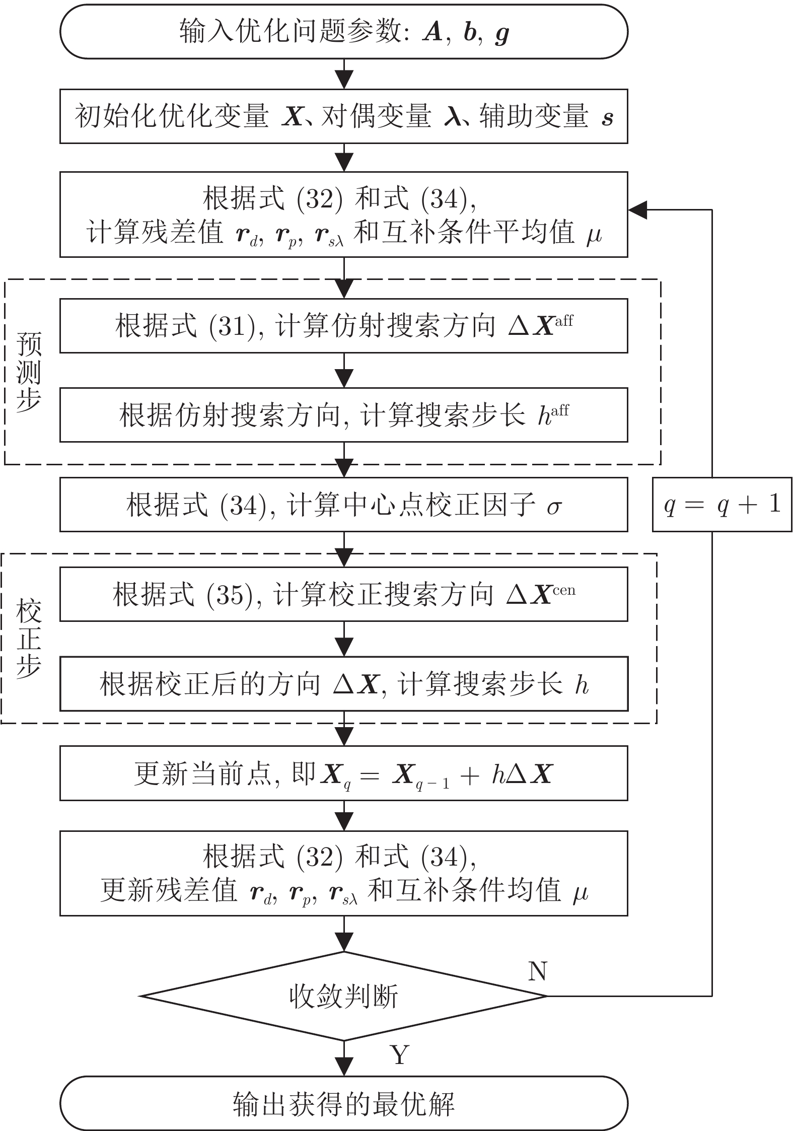
本文定制内点法的框架沿用文献[21]提出的预测−校正原对偶内点法, 其流程如图3所示, 包括初始化、预测步、校正步、搜索点更新和收敛判断等.
在预测−校正原对偶内点法的每次迭代中, 搜索点的更新需考虑预测步和校正步. 其中, 预测步通过求解牛顿系统计算仿射方向和步长; 校正步则利用仿射搜索信息对牛顿系统进行高阶修正, 然后求解获得校正搜索方向和步长, 以实现沿中心路径快速搜索最优解. 其中, 在确定搜索方向后, 搜索步长$h $根据Wolfe准则计算得到.
中心路径为严格可行点构成的一条曲线[21], 其定义为
$$F({{\boldsymbol{X}}_\tau },{{\boldsymbol{\lambda }}_\tau },{{\boldsymbol{s}}_\tau }) = \left[ {\begin{array}{*{20}{c}} {\boldsymbol{0}} \\ {\boldsymbol{0}} \\ {\tau {\boldsymbol{e}}} \end{array}} \right]$$ (27) 其中, $\tau $为中心路径参数. $F({\boldsymbol{X}},{\boldsymbol{\lambda }},{\boldsymbol{s}})\;$可根据式(26)表示为
$$F({\boldsymbol{X}},{\boldsymbol{\lambda }},{\boldsymbol{s}})\; = \left[ {\begin{array}{*{20}{c}} {{\boldsymbol{g}} + {{\boldsymbol{A}}^{\rm{T}}} \cdot {\boldsymbol{\lambda }}} \\ {{\boldsymbol{s}} + {\boldsymbol{A}} \cdot {\boldsymbol{X}} - {\boldsymbol{b}}} \\ {{\boldsymbol{S}}{\boldsymbol{\Lambda}} {\boldsymbol{e}}} \end{array}} \right]$$ (28) 其中, ${\boldsymbol{ \Lambda}} = {\rm{diag}}\{\boldsymbol{\lambda }\}$, ${\boldsymbol{S}} = {\rm{diag}}\{{\boldsymbol{s}}\}$, ${\boldsymbol{e}} = [1, 1,\cdots,1]^{\rm{T}}$.
4.2 原对偶搜索方向计算公式
在预测−校正原对偶内点法中, 搜索方向$\Delta {\boldsymbol{X}}$由预测步搜索方向$\Delta {{\boldsymbol{X}}^{{\rm{aff}}}}$和中心校正方向$\Delta {{\boldsymbol{X}}^{{\rm{cen}}}}$构成, 如式(29)所示[21].
$$\Delta {\boldsymbol{X}}=\Delta {{\boldsymbol{X}}^{{\rm{aff}}}} + \Delta {{\boldsymbol{X}}^{{\rm{cen}}}}$$ (29) 其中, 上标aff表示预测步的参数取值, 上标cen表示校正步的参数取值. $\Delta {{\boldsymbol{X}}^{{\rm{aff}}}}$和$\Delta {{\boldsymbol{X}}^{{\rm{cen}}}}$的计算方法如下所述.
1)预测步搜索方向
在预测步, 直接利用牛顿法计算迭代方向, 即计算函数$F({\boldsymbol{X}},{\boldsymbol{\lambda }},{\boldsymbol{s}})$的雅可比矩阵$J({\boldsymbol{X}},{\boldsymbol{\lambda }},{\boldsymbol{s}})$, 构建非线性方程组的牛顿系统, 具体为
$$J({{\boldsymbol{X}}_q},{{\boldsymbol{\lambda }}_q},{{\boldsymbol{s}}_q})\left[ {\begin{array}{*{20}{c}} {\Delta {{\boldsymbol{X}}_q}} \\ {\Delta {{\boldsymbol{\lambda }}_q}} \\ {\Delta {{\boldsymbol{s}}_q}} \end{array}} \right] = - F({{\boldsymbol{X}}_q},{{\boldsymbol{\lambda }}_q},{{\boldsymbol{s}}_q})$$ (30) 其中, 下标q表示内点法中当前的迭代步数.
因此, 预测步的搜索方向$\Delta {{\boldsymbol{X}}^{{\rm{aff}}}}$可根据式(31)计算得到:
$$\left[ {\begin{array}{*{20}{c}} {\boldsymbol{0}}&{{{\boldsymbol{A}}^{\rm{T}}}}&{\boldsymbol{0}} \\ {\boldsymbol{A}}&{\boldsymbol{0}}&{\boldsymbol{I}} \\ {\boldsymbol{0}}&{\boldsymbol{S}}&{\boldsymbol{\Lambda}} \end{array}} \right]\left[ {\begin{array}{*{20}{c}} {\Delta {{\boldsymbol{X}}^{{\rm{aff}}}}} \\ {\Delta {{\boldsymbol{\lambda }}^{{\rm{aff}}}}} \\ {\Delta {{\boldsymbol{s}}^{{\rm{aff}}}}} \end{array}} \right] = - \left[ {\begin{array}{*{20}{c}} {{{\boldsymbol{r}}_d}} \\ {{{\boldsymbol{r}}_p}} \\ {{{\boldsymbol{r}}_{s\lambda }}} \end{array}} \right]$$ (31) 其中, $\Delta {\boldsymbol{\lambda }}$和$\Delta {\boldsymbol{s}}$表示拉格朗日乘子${\boldsymbol{\lambda}}$和辅助变量s对应的搜索方向; 右端项的对偶残差rd, 原残差${{\boldsymbol{r}}_p} $和互补残差${{{\boldsymbol{r}}_{s\lambda }}} $可将第q次迭代步的值$({{\boldsymbol{X}}_q},{{\boldsymbol{\lambda }}_q}, {{\boldsymbol{s}}_q})$代入式(28)计算得到:
$$\left[ {\begin{array}{*{20}{c}} {{{\boldsymbol{r}}_d}} \\ {{{\boldsymbol{r}}_p}} \\ {{{\boldsymbol{r}}_{s\lambda }}} \end{array}} \right] = \left[ {\begin{array}{*{20}{c}} {{\boldsymbol{g}} + {{\boldsymbol{A}}^{\rm{T}}} \cdot {{\boldsymbol{\lambda }}_q}} \\ {{{\boldsymbol{s}}_q} + {\boldsymbol{A }}\cdot {{\boldsymbol{X}}_q} - {\boldsymbol{b}}} \\ {{{\boldsymbol{S}}_q}{{\boldsymbol{\Lambda}} _q}{\boldsymbol{e}}} \end{array}} \right]$$ (32) 2)校正步搜索方向
预测搜索方向是对非线性系统线性化计算得到的仿射方向, 为了使迭代能够贴近中心路径和加快迭代收敛, 增加校正步以修正仿射搜索方向.
由于式(26)的前两项均为仿射方程, 因此校正步仅需对最优条件的第3项进行校正, 校正后的互补残差${{\boldsymbol{r}}'_{s\lambda }}$可表示为
$$ - {{\boldsymbol{r}}'_{s\lambda }} = - {{\boldsymbol{r}}_{s\lambda }} - \Delta {{\boldsymbol{s}}^{{\rm{aff}}}}\Delta {{\boldsymbol{\Lambda}} ^{{\rm{aff}}}}{\boldsymbol{e}}{\rm{ + }}\sigma \mu {\boldsymbol{e}}$$ (33) 其中, $\sigma \in \left( {0,1} \right)$为中心校正因子, $\mu $为互补条件均值, 其表达式为
$$\sigma = \left(\frac{{\mu ^{{\rm{aff}}}}}{\mu }\right)^3,\;\;\;\mu = \frac{{{\boldsymbol{\lambda }}^{\rm{T}}}{\boldsymbol{s}}}{{n_A}}$$ (34) 基于校正后的残差值, 校正步的搜索方向$\Delta {{\boldsymbol{X}}^{{\rm{cen}}}}$可根据式(35)进行计算:
$$\left[ {\begin{array}{*{20}{c}} {\boldsymbol{0}}&{{{\boldsymbol{A}}^{\rm{T}}}}&{\boldsymbol{0}} \\ {\boldsymbol{A}}&{\boldsymbol{0}}&{\boldsymbol{I}} \\ {\boldsymbol{0}}&{\boldsymbol{S}}&{\boldsymbol{\Lambda}} \end{array}} \right]\left[ {\begin{array}{*{20}{c}} {\Delta {{\boldsymbol{X}}^{{\rm{cen}}}}} \\ {\Delta {{\boldsymbol{\lambda }}^{{\rm{cen}}}}} \\ {\Delta {{\boldsymbol{s}}^{{\rm{cen}}}}} \end{array}} \right] = - \left[ {\begin{array}{*{20}{c}} {{{\boldsymbol{r}}_d}} \\ {{{\boldsymbol{r}}_p}} \\ {{{{\boldsymbol{r}}}'_{s\lambda }}} \end{array}} \right]$$ (35) 4.3 原对偶搜索方向快速计算方法
为了获得原对偶搜索方向, 预测步和校正步需要分别求解式(31)和式(35)所示的非线性方程组, 本节针对方程特点, 定制搜索方向的快速计算方法.
1)逐次消元求解搜索方向
若直接对方程组的左端矩阵进行求逆, 由于矩阵非对称且不正定, 迭代过程中容易发生矩阵奇异, 导致内点法迭代难以收敛.
对此, 本研究通过逐次消元推导, 定制非线性方程组的求解步骤, 避免求解过程出现非对称矩阵求逆运算, 而且变量逐次求解可以降低计算复杂性.
针对预测步搜索方向的计算, 首先根据式(31)的第3行, 推导可得
$$\Delta {{\boldsymbol{s}}^{{\rm{aff}}}} = - {{\boldsymbol{\Lambda}} ^{ - 1}} \cdot {{\boldsymbol{r}}_{s\lambda }} - {{\boldsymbol{\Lambda}} ^{ - 1}} \cdot {\boldsymbol{S}} \cdot \Delta {{\boldsymbol{\lambda }}^{{\rm{aff}}}}$$ (36) 将式(36)与式(31)第2行结合, 消去$\Delta {{\boldsymbol{s}}^{{\rm{aff}}}}$, 可得
$$\Delta {{\boldsymbol{\lambda }}^{{\rm{aff}}}} = \left( {{{\boldsymbol{S}}^{ - 1}} \cdot {\boldsymbol{\Lambda}} } \right) \cdot \left( {{\boldsymbol{A}} \cdot \Delta {{\boldsymbol{X}}^{{\rm{aff}}}} + {{\boldsymbol{r}}_p} - {{\boldsymbol{\Lambda}} ^{ - 1}} \cdot {{\boldsymbol{r}}_{s\lambda }}} \right)$$ (37) 再将式(37)与式(31)第1行结合, 消去$\Delta {{\boldsymbol{\lambda }}^{{\rm{aff}}}}$可得
$$\begin{split} \Delta {{\boldsymbol{X}}^{{\rm{aff}}}}=\;&{\left[ {{{\boldsymbol{A}}^{\rm{T}}}\left( {{{\boldsymbol{S}}^{ - 1}} \cdot {\boldsymbol{\Lambda}} } \right) \cdot {\boldsymbol{A}}} \right]^{ - 1}}\; \cdot \\ &\left[ { - {{\boldsymbol{r}}_d} - {{\boldsymbol{A}}^{\rm{T}}} \cdot {{\boldsymbol{S}}^{ - 1}} \cdot \left( {{\boldsymbol{\Lambda}} \cdot {{\boldsymbol{r}}_p} - {{\boldsymbol{r}}_{s\lambda }}} \right)} \right] \end{split}$$ (38) 通过上述推导, 将根据式(31)对变量同时求解的方式转换为依次根据式(38)、(37)和(36)求解$\Delta {{\boldsymbol{X}}^{{\rm{aff}}}}$、$\Delta {{\boldsymbol{\lambda }}^{{\rm{aff}}}}$和$\Delta {{\boldsymbol{s}}^{{\rm{aff}}}}$.
采用相同的消元方式, 可以得到校正步方向的计算公式, 即
$$\begin{split} \Delta {{\boldsymbol{X}}^{{\rm{cen}}}}=&{\left[ {{{\boldsymbol{A}}^{\rm{T}}}\left( {{{\boldsymbol{S}}^{ - 1}} \cdot {\boldsymbol{\Lambda}} } \right) \cdot {\boldsymbol{A}}} \right]^{ - 1}}\;\cdot \\ & \left[ { - {{\boldsymbol{r}}_d} - {{\boldsymbol{A}}^{\rm{T}}} \cdot {{\boldsymbol{S}}^{ - 1}} \cdot \left( {{\boldsymbol{\Lambda}} \cdot {{\boldsymbol{r}}_p} - {{{\boldsymbol{r}}'}_{s\lambda }}} \right)} \right] \\ \Delta {{\boldsymbol{\lambda }}^{{\rm{cen}}}} =& \left( {{{\boldsymbol{S}}^{ - 1}} \cdot {\boldsymbol{\Lambda}} } \right) \cdot \left( {{\boldsymbol{A}} \cdot \Delta {\boldsymbol{X}} + {{\boldsymbol{r}}_p} - {{\boldsymbol{\Lambda}} ^{ - 1}} \cdot {{{\boldsymbol{r}}'}_{s\lambda }}} \right) \\ \Delta {{\boldsymbol{s}}^{{\rm{cen}}}} =& - {{\boldsymbol{\Lambda}} ^{ - 1}} \cdot {{{\boldsymbol{r}}'}_{s\lambda }} - {{\boldsymbol{\Lambda}} ^{ - 1}} \cdot {\boldsymbol{S}} \cdot \Delta {\boldsymbol{\lambda }} \\[-10pt] \end{split} $$ (39) 2)基于LDL分解降低计算复杂度
依据前述的消元逐次求解方法, 原对偶搜索方向的计算量主要在${{\boldsymbol{A}}^{\rm{T}}}\left( {{{\boldsymbol{S}}^{ - 1}} \cdot {\boldsymbol{\Lambda}} } \right) \cdot {\boldsymbol{A}}$的求逆运算. 由于${\boldsymbol{S}}$和${\boldsymbol{\Lambda}}$均为对角矩阵, 所以${{\boldsymbol{S}}^{ - 1}} \cdot {\boldsymbol{\Lambda}}$为对角矩阵. 结合式(22)中${\boldsymbol{A}} $的表达式, 可将${{\boldsymbol{S}}^{ - 1}} \cdot{\boldsymbol{ \Lambda }}$表示为
$${{\boldsymbol{S}}^{ - 1}} \cdot {\boldsymbol{\Lambda}} = \left[ {\begin{array}{*{20}{c}} {{{\boldsymbol{D}}_1}}&{}&{}&{}&{} \\ {}&{{{\boldsymbol{D}}_2}}&{}&{}&{} \\ {}&{}&{{{\boldsymbol{D}}_3}}&{}&{} \\ {}&{}&{}&{{{\boldsymbol{D}}_4}}&{} \\ {}&{}&{}&{}&{{{\boldsymbol{D}}_5}} \end{array}} \right]$$ (40) 其中, ${{\boldsymbol{D}}_1} \in {{\bf{R}}^{{n_{{\rm{tr}}}} \times {n_{{\rm{tr}}}}}}$, ${{\boldsymbol{D}}_2} \in {{\bf{R}}^{{n_{{\rm{eq}}}} \times {n_{{\rm{eq}}}}}}$, ${{\boldsymbol{D}}_3} \in {{\bf{R}}^{{n_{{\rm{eq}}}} \times {n_{{\rm{eq}}}}}}$, ${{\boldsymbol{D}}_4} \in {{\bf{R}}^{{n_{{\rm{in}}}} \times {n_{{\rm{in}}}}}}$, ${{\boldsymbol{D}}_5} \in {{\bf{R}}^{{n_{{\rm{in}}}} \times {n_{{\rm{in}}}}}}$均为对角矩阵.
根据式(22), 计算可得${{\boldsymbol{A}}^{\rm{T}}}\left( {{{\boldsymbol{S}}^{ - 1}} \cdot {\boldsymbol{\Lambda }}} \right)\cdot{\boldsymbol{A}}$为
$${{\boldsymbol{A}}^{\rm{T}}}\left( {{{\boldsymbol{S}}^{ - 1}} \cdot {\boldsymbol{\Lambda }}} \right)\cdot{\boldsymbol{A}} = \left[ {\begin{array}{*{20}{c}} {{{\boldsymbol{\Gamma}} _{11}}}&{{{\boldsymbol{\Gamma}} _{12}}}&{{{\boldsymbol{\Gamma}} _{13}}} \\ {{\boldsymbol{\Gamma }}_{12}^{\rm{T}}}&{{{\boldsymbol{D}}_2} + {{\boldsymbol{D}}_3}}&{\boldsymbol{0}} \\ {{\boldsymbol{\Gamma }}_{13}^{\rm{T}}}&{\boldsymbol{0}}&{{{\boldsymbol{D}}_4} + {{\boldsymbol{D}}_5}} \end{array}} \right]$$ (41) 其中,
$$\begin{split} & {{\boldsymbol{\Gamma}} _{11}}={\boldsymbol{A}}_{{\rm{tr}}}^{\rm{T}}{{\boldsymbol{D}}_1}{{\boldsymbol{A}}_{{\rm{tr}}}} + {\boldsymbol{A}}_{{\rm{eq}}}^{\rm{T}}{{\boldsymbol{D}}_2}{{{\boldsymbol{A}}_{{\rm{eq}}}}}\;+ \\ & \;\;\;\qquad {\boldsymbol{A}}_{{\rm{eq}}}^{\rm{T}}{{\boldsymbol{D}}_3}{{{\boldsymbol{A}}_{{\rm{eq}}}}} + {\boldsymbol{A}}_{{\rm{in}}}^{\rm{T}}{{\boldsymbol{D}}_4}{{\boldsymbol{A}}_{{\rm{in}}}} \\ & {{\boldsymbol{\Gamma}} _{12}}={\boldsymbol{A}}_{{\rm{eq}}}^{\rm{T}}({{\boldsymbol{D}}_3} - {{\boldsymbol{D}}_2}) \\ & {{\boldsymbol{\Gamma}} _{13}}= - {\boldsymbol{A}}_{{\rm{in}}}^{\rm{T}}{{\boldsymbol{D}}_4} \end{split}$$ (42) 对于多无人机协同轨迹规划问题, 由式(5) ~ (12)可知, 矩阵${\boldsymbol{A}}_{\rm{eq}} $、${\boldsymbol{A}}_{\rm{in}} $和${\boldsymbol{A}}_{\rm{tr}} $均为稀疏矩阵, 其中${\boldsymbol{A}}_{\rm{eq}} $为分块双对角与列向量组合的形式, 如式(43)所示.
$${{{\boldsymbol{A}}_{{\rm{eq}}}}} = \left[ {\begin{array}{*{20}{c}} {{{\boldsymbol{A}}_{0,0}}} &{}&{}&{}&{}&{{{\boldsymbol{a}}_0}} \\ {{{\boldsymbol{A}}_{1,0}}} & {{{\boldsymbol{A}}_{1,1}}}&{}&{}&{}&{{{\boldsymbol{a}}_1}} \\ {}&{{{\boldsymbol{A}}_{2,1}}} & {{{\boldsymbol{A}}_{2,2}}}&{}&{}&{{{\boldsymbol{a}}_2}} \\ {}&{}& \ddots & \ddots &{}& \vdots \\ {}&{} &{}& {{{\boldsymbol{A}}_{K,K - 1}}}& {{{\boldsymbol{A}}_{K,K}}}& {{{\boldsymbol{a}}_K}} \\ {}&{}&{}&{} & {{{\boldsymbol{A}}_{K + 1,K}}}& {{{\boldsymbol{a}}_{K + 1}}} \end{array}} \right]$$ (43) ${\boldsymbol{A}}_{\rm{in}} $中的避障约束、避碰约束、状态边界约束以及信赖域约束系数矩阵${\boldsymbol{A}}_{\rm{tr}} $均为分块对角矩阵, 例如信赖域约束的左端项系数矩阵形式如式(44)所示.
$${{\boldsymbol{A}}_{{\rm{tr}}}} = \left[ {\begin{array}{*{20}{c}} {{{\boldsymbol{A}}_0}}&{}&{}&{}\\ {}&{{{\boldsymbol{A}}_1}}&{}&{}\\ {}&{}& \ddots &{}\\ {}&{}&{}&{{{\boldsymbol{A}}_K}} \end{array}} \right]$$ (44) 同时, 考虑到矩阵${\boldsymbol{D}}_1,{\boldsymbol{D}}_2,\cdots,{\boldsymbol{D}}_5 $均为对角矩阵, 因此, ${{\boldsymbol{A}}^{\rm{T}}}\left( {{{\boldsymbol{S}}^{ - 1}} \cdot {\boldsymbol{\Lambda}} } \right) \cdot {\boldsymbol{A}}$为稀疏的对称矩阵. 对此, 可以采用稀疏矩阵的LDL分解[22], 即
$${\boldsymbol{P}} \cdot \left( {{{\boldsymbol{A}}^{\rm{T}}}\left( {{{\boldsymbol{S}}^{ - 1}} \cdot{\boldsymbol{ \Lambda}} } \right) \cdot {\boldsymbol{A}}} \right) \cdot {{\boldsymbol{P}}^{\rm{T}}}={\boldsymbol{L}} \cdot{\boldsymbol{ D}} \cdot {{\boldsymbol{L}}^{\rm{T}}}$$ (45) 其中, P为排列矩阵, L为单位下三角矩阵, D为分块对角阵. 则式(38)可以转化为
$$\begin{split} & \left( {{{\boldsymbol{P}}^{\rm{T}}} \cdot {\boldsymbol{L}} \cdot {\boldsymbol{D}} \cdot {{\boldsymbol{L}}^{\rm{T}}} \cdot {\boldsymbol{P}}} \right) \cdot \Delta {{\boldsymbol{X}}^{{\rm{aff}}}}= \\ &\qquad\left[ { - {{\boldsymbol{r}}_d} - {{\boldsymbol{A}}^{\rm{T}}} \cdot {{\boldsymbol{S}}^{ - 1}} \cdot \left( {{\boldsymbol{\Lambda}} \cdot {{\boldsymbol{r}}_p} - {{\boldsymbol{r}}_{s\lambda }}} \right)} \right] \end{split}$$ (46) 从而, 可将求解搜索方向$\Delta {{\boldsymbol{X}}^{{\rm{aff}}}}$转化为求解一系列低计算成本的方程, 计算过程如式(47)所示. 而且计算校正搜索方向$\Delta {{\boldsymbol{X}}^{{\rm{cen}}}}$时, 可用同样的方法降低计算成本.
$$ \begin{split} &{\boldsymbol{L}} \cdot {\boldsymbol{u}}={\boldsymbol{P}} \cdot \left[ { - {{\boldsymbol{r}}_d} - {{\boldsymbol{A}}^{\rm{T}}}{{\boldsymbol{S}}^{ - 1}}\left( {{\boldsymbol{\Lambda}} \cdot {{\boldsymbol{r}}_p} - {{\boldsymbol{r}}_{s\lambda }}} \right)} \right] \Rightarrow {\boldsymbol{u}} \\ &{\boldsymbol{D}} \cdot {\boldsymbol{v}} = {\boldsymbol{u}}\;\; \Rightarrow {\boldsymbol{v}} \\ &{{\boldsymbol{L}}^{\rm{T}}} \cdot {\boldsymbol{w}} = {\boldsymbol{v}}\; \Rightarrow {\boldsymbol{w}} \\ &{\boldsymbol{P}} \cdot \Delta {{\boldsymbol{X}}^{{\rm{aff}}}} \Rightarrow \Delta {{\boldsymbol{X}}^{{\rm{aff}}}} \end{split} $$ (47) 为了说明定制方法计算搜索方向的优势, 以浮点运算次数为统计指标, 对下述3种方式的计算复杂度进行定量分析: 方法I (即定制方法)通过LDL分解计算$\Delta {\boldsymbol{X}}$, 再依次计算$\Delta {\boldsymbol{\lambda }}$和$\Delta {\boldsymbol{s}}$; 方法II以求逆方式求解式(38), 再计算$\Delta {\boldsymbol{\lambda }}$和$\Delta {\boldsymbol{s}}$; 方法III直接以求逆方式求解式(31). 3种方法的计算成本如表1所示, 其中, ${n_X}$和${n_A}$的表达式见式(23).
表 1 原对偶搜索方向计算复杂度Table 1 Computation complexity for primal-dual search direction计算方法 计算成本 方法 I 0.33$n_{{X}}^3$+ 3$n_A^3$+$n_{{X}}^2{n_A}$+${n_{{X}}}n_A^2$ 方法 II 2.67$n_{{X}}^3$+ 3$n_A^3$+$n_{{X}}^2{n_A}$+${n_{{X}}}n_A^2$ 方法III 2.67 (${n_{{X}}}$+2${n_A}$)3 图4给出了3种搜索方向生成方法的计算复杂度随变量维度nX和约束数量nA的变化情况. 由表1和图4可见, 本文提出的定制方法通过消元逐次计算(比较方法III和方法II)和LDL分解(比较方法II和方法I)减少了原对偶搜索方向的计算复杂度, 从而可以降低子问题优化成本.
 图 4 原对偶搜索方向计算复杂度变化图Fig. 4 Variations of computation complexity for primal-dual search direction
另外, 上述定制算法利用数值特征降低子问题的计算成本, 并不会改变原对偶内点法或SCP协同轨迹规划的收敛性, 其收敛性分析可参考文献[4]和文献[23-24].
5. 仿真实验
本节通过数值仿真实验, 在解耦SCP协同轨迹规划架构下, 验证定制内点法的有效性, 并将定制内点法与一般内点法进行对比, 验证定制内点法的性能优势.
5.1 仿真环境与想定
数值仿真实验在Windows7中的MATLAB 2016a下进行, 硬件环境为Intel Core i5-2310@2.90 GHz处理器和4 GB内存的PC机. 凸优化子问题分别利用定制内点法和SeDuMi[17]进行对比求解. SeDuMi是广泛应用于MATLAB环境的一种凸优化工具包, 其中采用了基本的预测−校正原对偶内点法, 因此将其作为对比算法以验证本文方法的性能.
采用文献[15]的仿真实验算例, 考虑7架无人机所构编队的集结和重构任务, 对本文提出的定制内点法进行测试验证. 无人机起始点、目标点和障碍的水平位置见仿真结果图, 无人机的起始点和目标点高度均设为400 m, 障碍半径均设为400 m. 编队飞行过程中, 无人机间的防撞安全距离设为100 m.
无人机初始时刻和终端时刻的速度、航向角和航迹倾角分别设为35 m/s, 0 rad和0 rad. 无人机状态量和控制量的边界约束为
$$\begin{split} & {{\boldsymbol{s}}_{i,\min }} = ( - \infty , - \infty ,300\;{\rm{m}},30\;{{\rm{m}}/{\rm{s}}}, - \infty ,{{ - 5\pi }/{180}}) \\ & {{\boldsymbol{s}}_{i,\max }} = ({\rm{ + }}\infty ,{\rm{ + }}\infty ,500\;{\rm{m}},40\;{{\rm{m}}/{\rm{s}}},{\rm{ + }}\infty ,{{ + 5\pi }/{180}}) \\ & {{\boldsymbol{u}}_{i,\min }} = {({\rm{ - 0}}{\rm{.2, - 0}}{\rm{.2,0}}{\rm{.8}})^{\rm{T}}}\\ &{{\boldsymbol{u}}_{i,{\rm{max}}}} = {(0.2,0.2,1.2)^{\rm{T}}} \\[-10pt] \end{split} $$ (48) 针对上述编队集结和重构想定, SCP算法相关参数设置为
$$\begin{split} &K = 40,\;\;\;\;\;\;\mu = 1\;000\;\; \\ & {\boldsymbol{\rho }} = {\left( {4\;000\;{\rm{m}},4\;000\;{\rm{m}},100\;{\rm{m}},20\;{{\rm{m}}/{\rm{s}}},\pi ,{\pi /{10}}} \right)^{\rm{T}}} \\ & {\boldsymbol{\varepsilon}} = {\left( {0.1,0.1,0.05,0.01,{{0.05\pi }/{180}},{{0.01\pi }/{180}}} \right)^{\rm{T}}} \end{split} $$ (49) 5.2 仿真结果与分析
1)定制内点法有效性测试
针对设定的7架无人机编队集结和重构任务, 基于定制内点法进行轨迹规划求解, 轨迹结果分别如图5和图6以及图7和图8所示. 由图可知, 定制内点法生成的无人机协同轨迹能够对飞行空间中的障碍进行有效规避, 并实现从初始点到给定集结点或队形重构点的平滑转移. 距离目标点较近的无人机进行了绕远飞行, 以实现飞行时间协同.
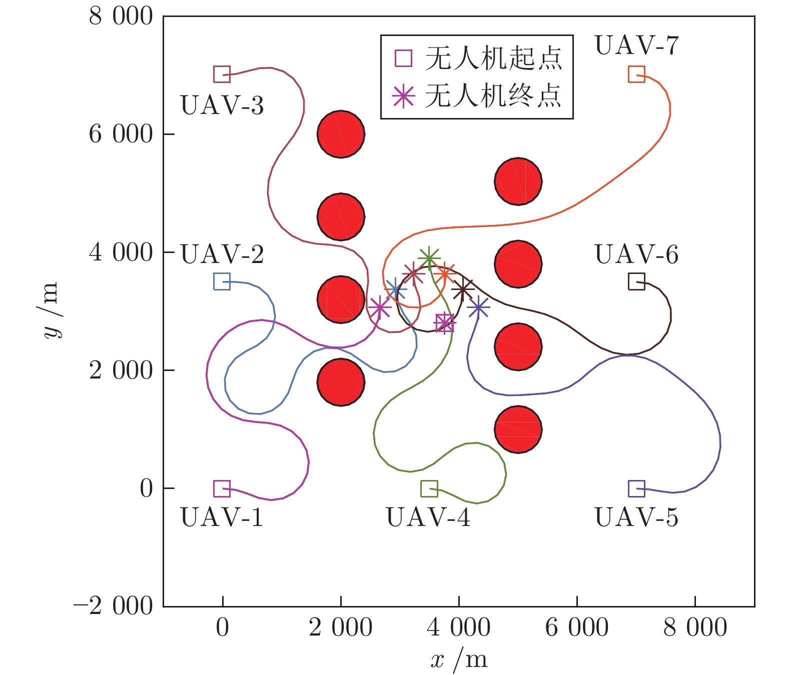
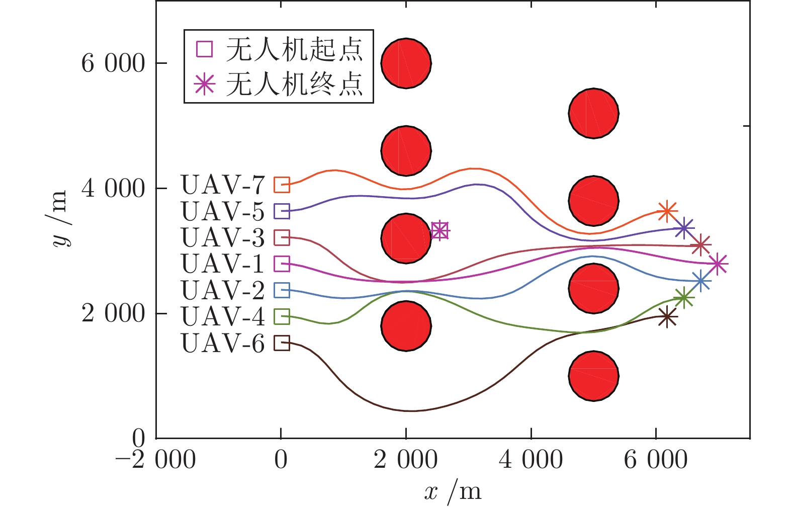 图 7 编队重构协同轨迹规划二维结果图Fig. 7 Cooperative trajectories in 2D for formation reconfiguration
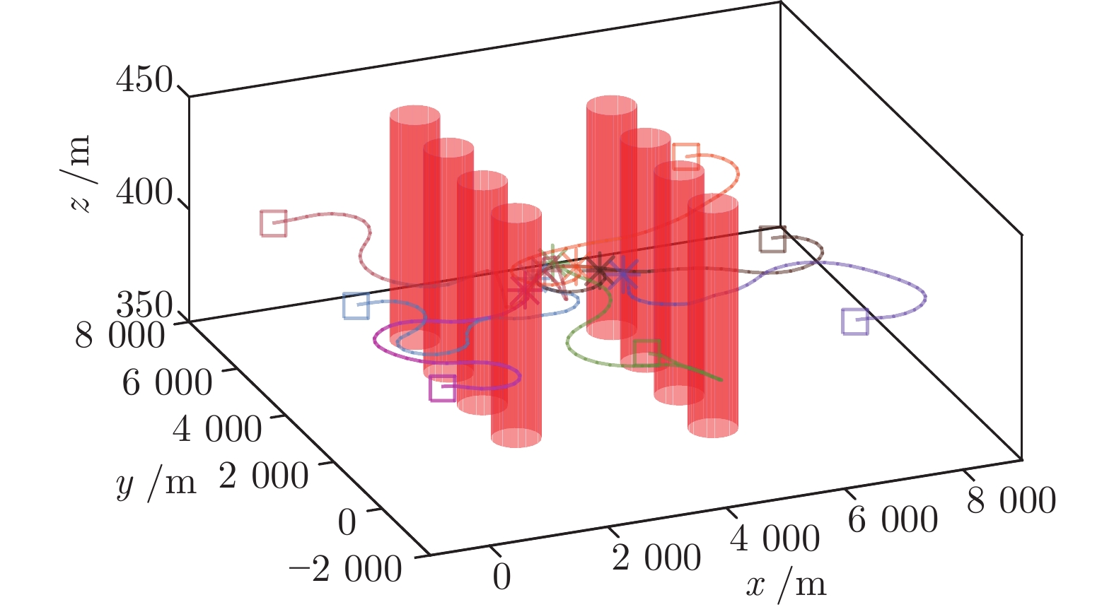
 图 8 编队重构协同轨迹规划三维结果图Fig. 8 Cooperative trajectories in 3D for formation reconfiguration
图9和图10给出了编队飞行过程中无人机间最短距离的变化曲线. 由图可知, 任意两架无人机间的距离始终大于设定的最小安全距离, 可见定制内点法生成的协同轨迹能够满足机间避碰约束, 实现空间协同.
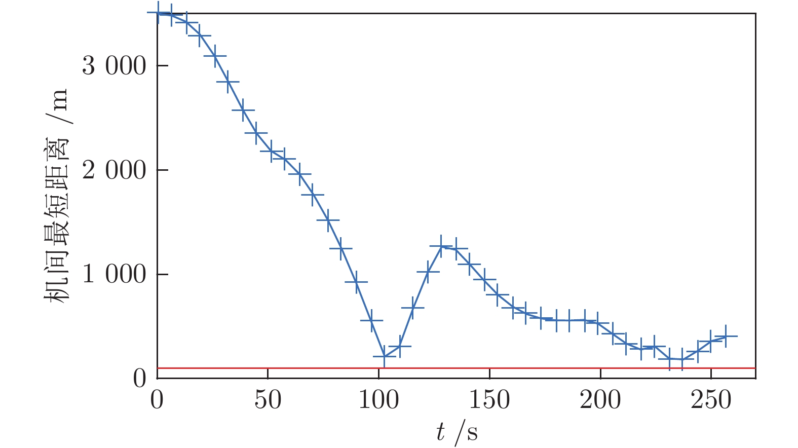 图 9 编队集结任务无人机间最短距离变化曲线Fig. 9 Variation curve of minimum distance between UAVs for formation rendezvous
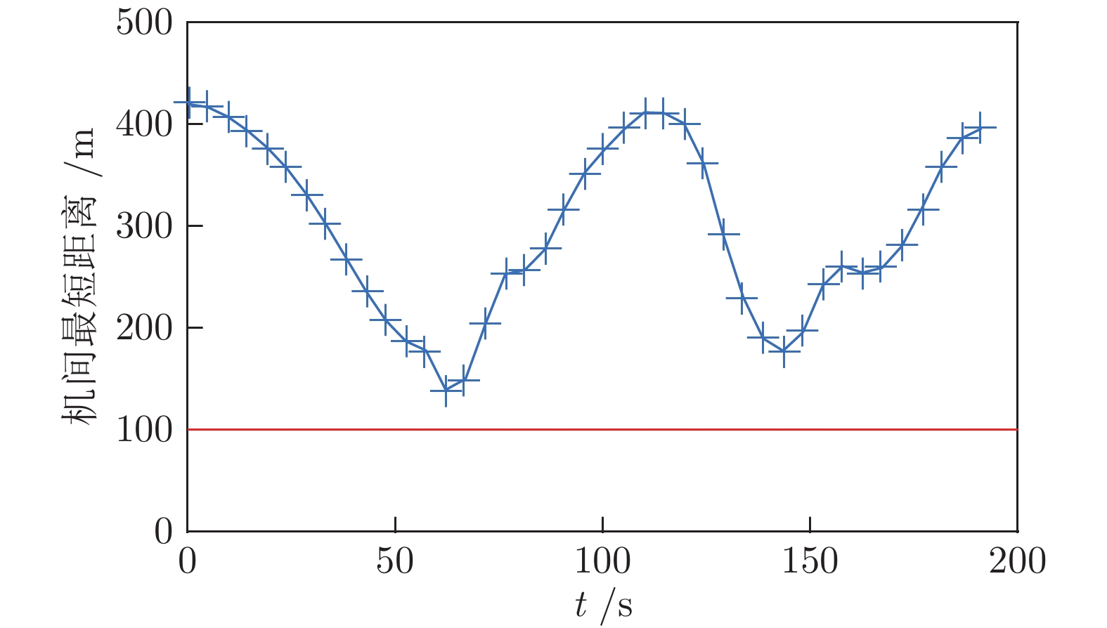 图 10 编队重构任务无人机间最短距离变化曲线Fig. 10 Variation curve of minimum distance between UAVs for formation reconfiguration
因此, 在解耦SCP框架下, 采用定制内点法对凸优化子问题进行求解, 能够规划生成满足约束的无人机编队协同轨迹.
2)算法性能对比测试
在验证定制内点法有效性的基础上, 开展算法对比仿真实验, 比较定制内点法和SeDuMi工具包中一般内点法的轨迹规划性能. 针对编队集结和重构任务, 编队无人机数量由1逐渐增加至7, 子问题求解分别采用定制内点法和SeDuMi, 对获得的协同轨迹规划结果和计算耗时进行统计.
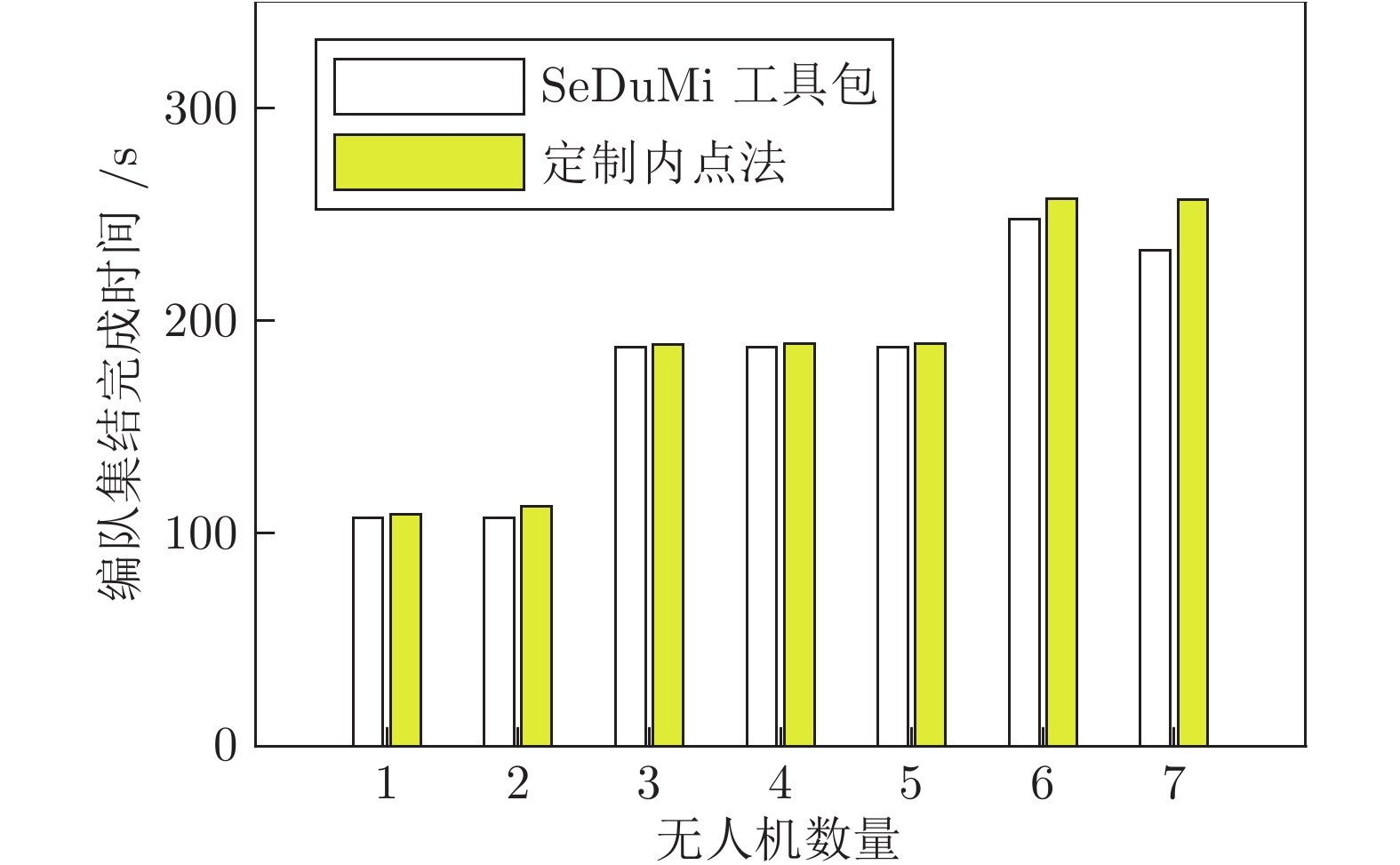
针对编队任务完成时间即飞行时间, 定制内点法和SeDuMi优化得到的编队集结时间如图11所示, 编队重构时间如图12所示. 不同编队规模下, SeDuMi获得的集结时间均值为179.67 s, 定制内点法为186.11 s, 两者相差约3.6%; SeDuMi获得的重构时间均值为187.34 s, 定制内点法为188.67 s, 两者相差约0.7%. 如式(1)所示, 本文以任务完成时间最短为优化目标, 因此定制内点法的寻优能力与SeDuMi基本相当.
针对7机编队集结任务, 图13和图14给出了SeDuMi和定制内点法规划结果对应的速度、高度和过载变化曲线. 根据7机集结平均速度统计结果, SeDuMi为34.27 m/s, 定制内点法为33.08 m/s. 这与图11中的7机集结时间结果相符, SeDuMi所得集结时间(232.86 s)少于定制方法(256.63 s).
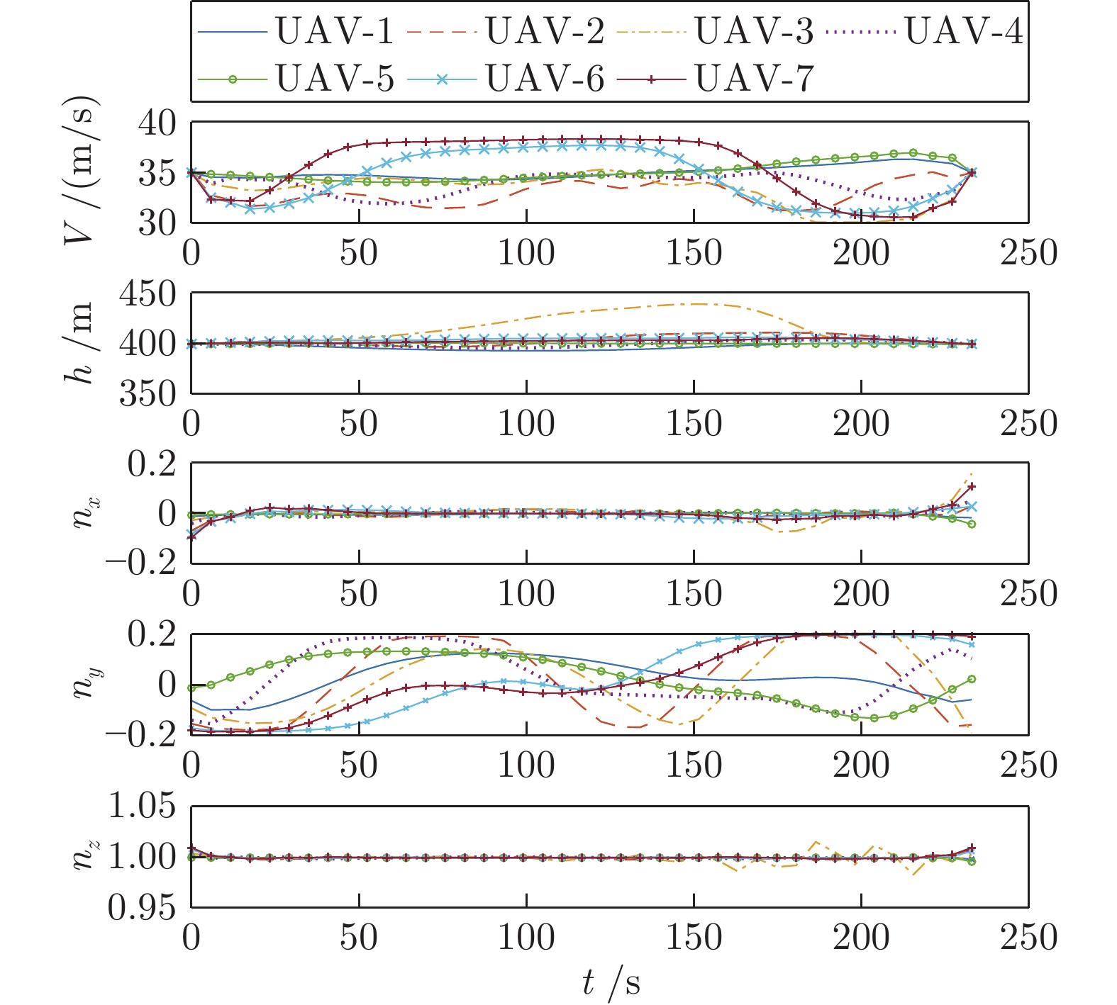 图 13 基于SeDuMi的编队集结轨迹规划结果Fig. 13 Trajectory planning results using SeDuMi for formation rendezvous
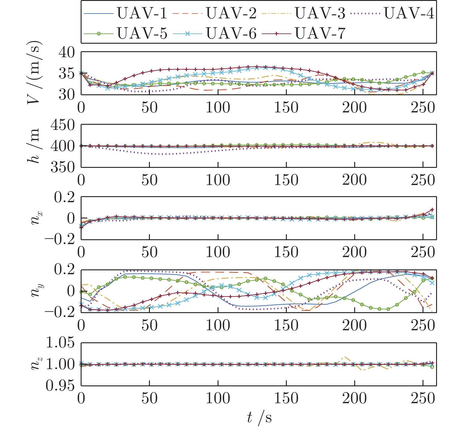 图 14 基于定制内点法的编队集结轨迹规划结果Fig. 14 Trajectory planning results using customized interior-point method for formation rendezvous
对无人机集结过程中速度和高度的标准差进行计算, 再统计获得编队的整体均值, 其中SeDuMi结果为1.78 m/s和4.33 m, 定制内点法结果为1.49 m/s和2.36 m. 可见定制内点法生成轨迹的状态变化稍平滑, 更易于轨迹跟踪控制, 但两者差距不大.
对无人机过载的绝对值之和进行统计, 该值可近似反映无人机控制能耗的大小关系. 其中铅垂方向以$(n_2-1) $进行统计. 根据统计, SeDuMi所得协同轨迹的三轴过载绝对值之和为(3.77, 33.04, 0.91), 定制内点法为(3.66, 37.30, 0.97). 可见, 两种方法所生成轨迹对应的控制能耗大小相当, 按定制内点法结果飞行所需的控制能耗略高.
图15和图16分别给出了7机编队重构想定下SeDuMi和定制内点法规划轨迹的速度、高度和过载变化曲线. SeDuMi生成轨迹的编队平均速度为35.71 m/s, 定制内点法则为36.08 m/s. 根据图12的7机编队重构时间结果, SeDuMi获得的重构时间(191.91 s)相应地也大于定制内点法结果(191.24 s).
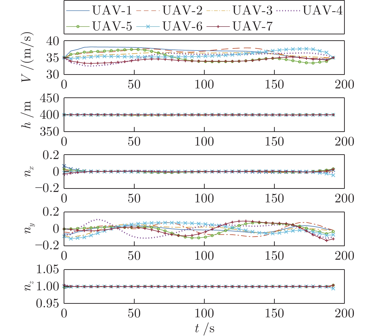 图 15 基于SeDuMi的编队重构轨迹规划结果Fig. 15 Trajectory planning results using SeDuMi for formation reconfiguration
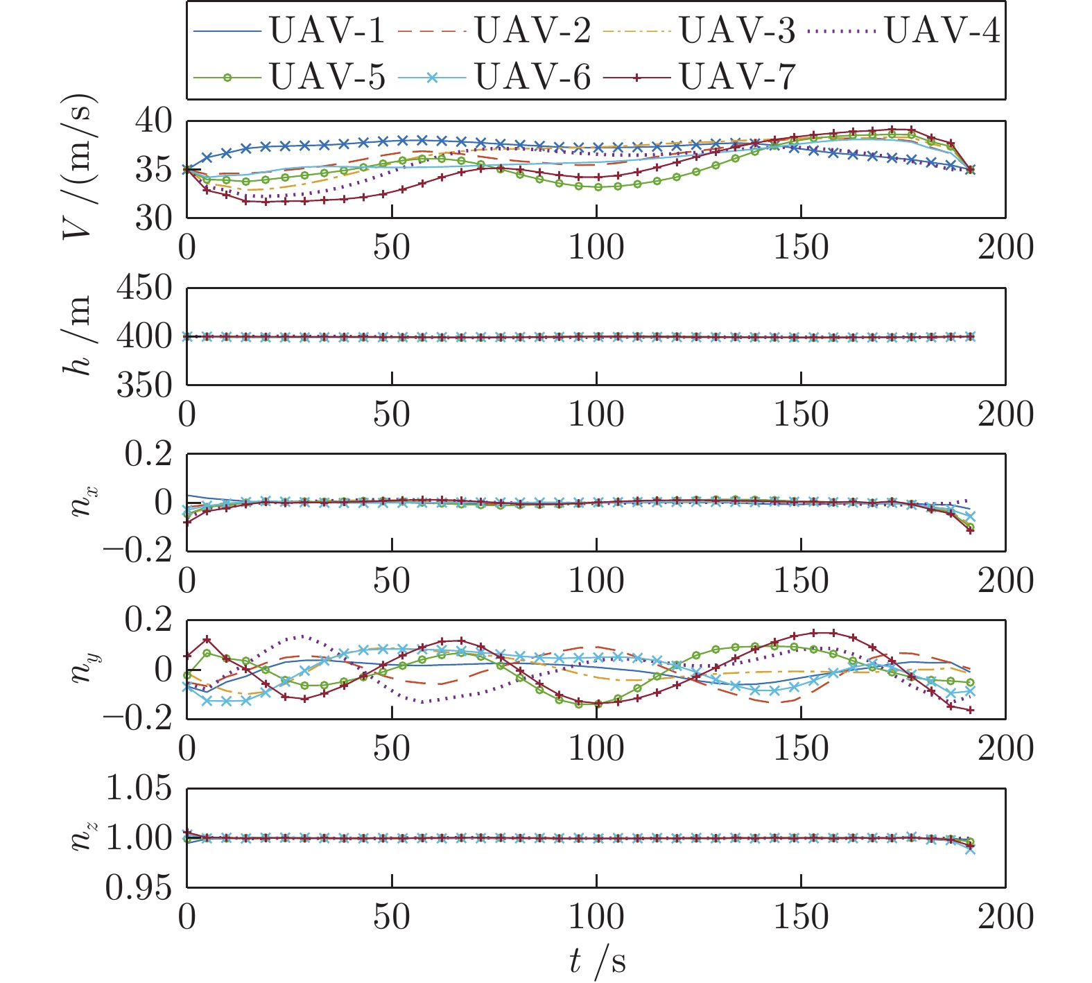 图 16 基于定制内点法的编队重构轨迹规划结果Fig. 16 Trajectory planning results using customized interior-point method for formation reconfiguration
根据编队无人机速度标准差和高度标准差的均值统计结果, SeDuMi为1.02 m/s和0.36 m, 定制内点法为1.64 m/s和0.34 m. 可见两种方法生成重构轨迹的平滑性相当, 都变化不大, 易于进行轨迹跟踪控制.
根据7机编队重构轨迹的过载统计结果, SeDuMi生成轨迹对应的三轴过载绝对值之和为(1.41, 13.84, 0.16), 定制内点法则为(2.72, 18.60, 0.33), 可见定制内点法所得轨迹对应的控制能耗略高于SeDuMi所得轨迹.
综合编队集结和重构的实验结果及分析, 在任务完成时间最优性、轨迹可实现性和轨迹控制能耗方面, 定制内点法所得轨迹结果与SeDuMi结果基本相当, 即两种方法在上述轨迹指标中相互不存在明显优势.
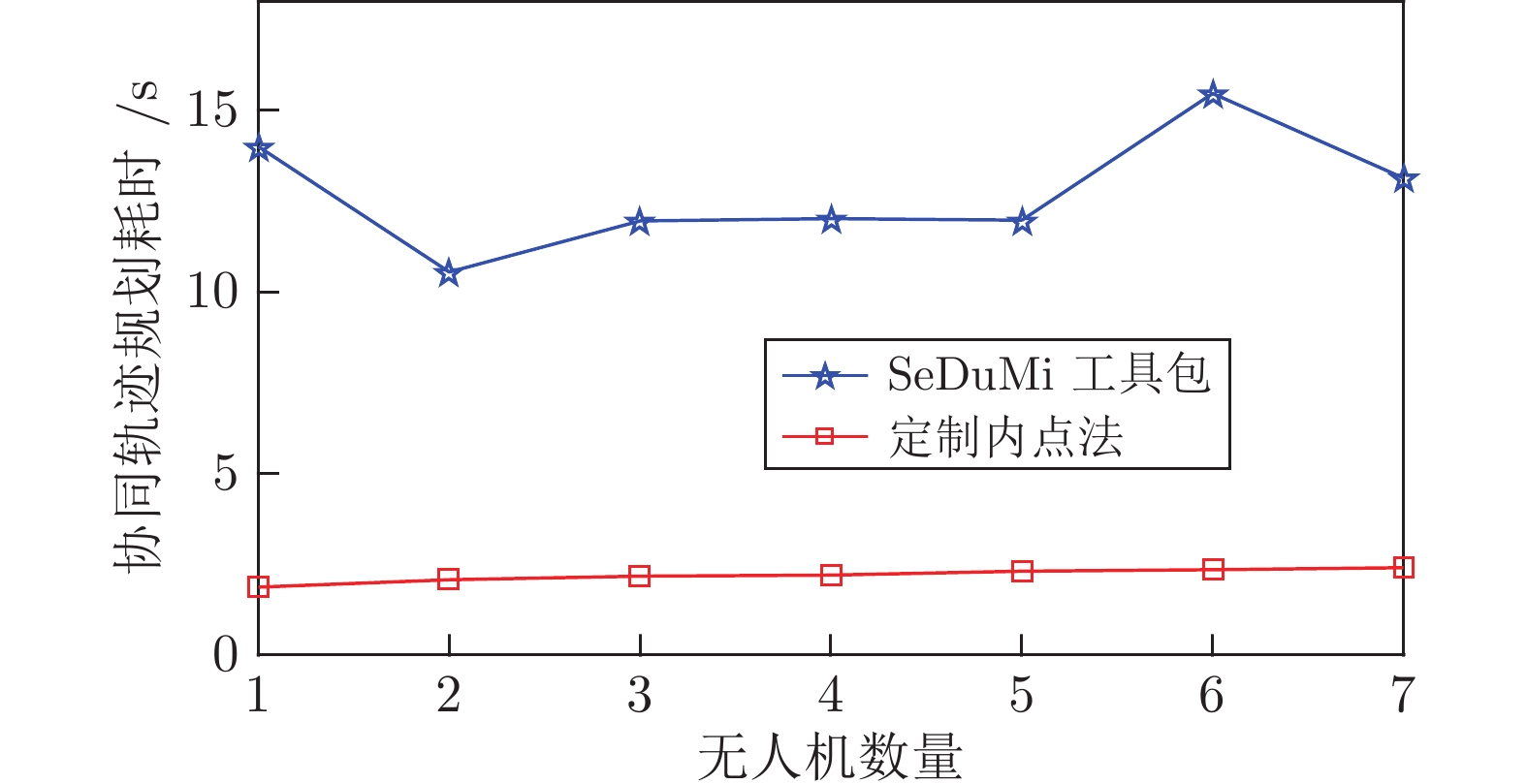
基于定制内点法和SeDuMi进行编队轨迹规划的计算耗时统计结果如图17和图18所示. 由图可见, 在所有想定下, 定制内点法的规划效率都优于SeDuMi. 其中, 对于7机集结和重构轨迹规划问题, 基于SeDuMi的轨迹规划耗时分别为19.0 s和13.1 s, 而基于定制内点法的耗时仅为3.0 s和2.4 s. 不同规模下编队集结和编队重构规划结果的统计数据表明, 基于定制内点法的轨迹规划平均耗时约为SeDuMi求解耗时的1/7和1/6.
同时, 对于上述编队集结和重构轨迹规划问题, 单机解耦规划时凸优化的变量维度nX和约束数量nA约为103和2×10³, 结合表1给出的计算复杂度表达式, 此时定制内点法在子优化问题求解时的计算复杂度约为一般内点法的1/10. 但除了子问题求解, 轨迹规划还需要完成子问题构建、协同约束生成等计算, 这些过程的计算耗时对于定制内点法和一般内点法是基本相同的. 因此, 定制内点法完成协同轨迹规划的耗时与一般内点法耗时的比值会大于1/10, 这与仿真实验获得的计算耗时统计结果是一致的.
另外, 根据文献[15]给出的伪谱法解耦协同轨迹规划结果, 上述编队集结和重构的平均计算耗时为100.7 s和111.0 s. 可见, 相比于广泛应用的伪谱法, 本文提出的定制内点法可显著提高轨迹规划的效率.
根据上述轨迹结果分析和计算时效性对比可知, 定制内点法生成的编队轨迹结果最优性与一般内点法相当, 但采用定制内点法可将协同轨迹规划的计算耗时降低一个数量级, 即从十秒级降低到秒级. 对于7机编队轨迹规划问题, 在解耦SCP规划架构下, 定制内点法可以在3 s内生成安全可行的编队协同轨迹.
6. 结束语
针对基于解耦SCP的多机协同轨迹规划中需迭代求解的凸优化子问题, 通过引入松弛变量构建等价形式, 并利用协同轨迹规划问题的模型特征, 定制子问题求解的高效内点法, 以降低子问题计算耗时, 进而提高协同轨迹规划效率. 在计算复杂度分析的基础上, 通过数值仿真对定制内点法的有效性和性能优势进行验证. 仿真结果表明, 在轨迹寻优能力、轨迹可实现性和轨迹控制能耗方面, 定制内点法可以获得与SeDuMi相当的轨迹结果, 但定制内点法完成轨迹规划的计算耗时相比SeDuMi可以降低一个数量级, 即由十秒级降至秒级.
-
图 1 多无人机协同轨迹规划问题示意图
Fig. 1 Illustration of multi-UAV cooperative trajectory planning problems
图 4 原对偶搜索方向计算复杂度变化图
Fig. 4 Variations of computation complexity for primal-dual search direction
图 7 编队重构协同轨迹规划二维结果图
Fig. 7 Cooperative trajectories in 2D for formation reconfiguration
图 8 编队重构协同轨迹规划三维结果图
Fig. 8 Cooperative trajectories in 3D for formation reconfiguration
图 9 编队集结任务无人机间最短距离变化曲线
Fig. 9 Variation curve of minimum distance between UAVs for formation rendezvous
图 10 编队重构任务无人机间最短距离变化曲线
Fig. 10 Variation curve of minimum distance between UAVs for formation reconfiguration
图 13 基于SeDuMi的编队集结轨迹规划结果
Fig. 13 Trajectory planning results using SeDuMi for formation rendezvous
图 14 基于定制内点法的编队集结轨迹规划结果
Fig. 14 Trajectory planning results using customized interior-point method for formation rendezvous
图 15 基于SeDuMi的编队重构轨迹规划结果
Fig. 15 Trajectory planning results using SeDuMi for formation reconfiguration
图 16 基于定制内点法的编队重构轨迹规划结果
Fig. 16 Trajectory planning results using customized interior-point method for formation reconfiguration
表 1 原对偶搜索方向计算复杂度
Table 1 Computation complexity for primal-dual search direction
计算方法 计算成本 方法 I 0.33$n_{{X}}^3$+ 3$n_A^3$+$n_{{X}}^2{n_A}$+${n_{{X}}}n_A^2$ 方法 II 2.67$n_{{X}}^3$+ 3$n_A^3$+$n_{{X}}^2{n_A}$+${n_{{X}}}n_A^2$ 方法III 2.67 (${n_{{X}}}$+2${n_A}$)3  下载: 导出CSV
-
[1] 沈林成, 牛轶峰, 朱华勇. 多无人机自主协同控制理论与方法. 北京: 国防工业出版社, 2013. 1−9Shen Lin-Cheng, Niu Yi-Feng, Zhu Hua-Yong. Theories and Methods of Autonomous Cooperative Control for Multiple UAVs. Beijing: National Defense Industry Press, 2013. 1−9 [2] Liu X F, Lu P, Pan B F. Survey of convex optimization for aerospace applications. Astrodynamics, 2017, 1(1): 23-40 doi: 10.1007/s42064-017-0003-8 [3] Boyd S, Vandenberghe L. Convex Optimization. Cambridge: Cambridge University Press, 2004. 1−15 [4] Liu X F, Lu P. Solving nonconvex optimal control problems by convex optimization. Journal of Guidance, Control, and Dynamics 2014, 37(3): 750-765 doi: 10.2514/1.62110 [5] Schulman J, Duan Y, Ho J, Lee A, Awwal I, Bradlow H, et al. Motion planning with sequential convex optimization and convex collision checking. The International Journal of Robotics Research, 2014, 33(9): 1251-1270 doi: 10.1177/0278364914528132 [6] Misra G, Bai X L. Optimal path planning for free-flying space manipulators via sequential convex programming. Journal of Guidance, Control, and Dynamics, 2017, 40(11): 3019-3026 doi: 10.2514/1.G002487 [7] 刘延杰, 朱圣英, 崔平远. 序列凸优化的小天体附着轨迹优化. 宇航学报, 2018, 39(2): 177-183 doi: 10.3873/j.issn.1000-1328.2018.02.008Liu Yan-Jie, Zhu Sheng-Ying, Cui Ping-Yuan. Soft landing trajectory optimization on asteroids by convex programming. Journal of Astronautics, 2018, 39(2): 177-183 doi: 10.3873/j.issn.1000-1328.2018.02.008 [8] 王劲博, 崔乃刚, 郭继峰, 徐大富. 火箭返回着陆问题高精度快速轨迹优化算法. 控制理论与应用, 2018, 35(3): 389-398 doi: 10.7641/CTA.2017.70730Wang Jin-Bo, Cui Nai-Gang, Guo Ji-Feng, Xu Da-Fu. High precision rapid trajectory optimization algorithm for launch vehicle landing. Control Theory & Applications, 2018, 35(3): 389-398 doi: 10.7641/CTA.2017.70730 [9] Zhang Z, Li J X, Wang J. Sequential convex programming for nonlinear optimal control problems in UAV path planning. Aerospace Science and Technology, 2018, 76: 280-290 doi: 10.1016/j.ast.2018.01.040 [10] Zhou D, Zhang Y Q, Li S L. Receding horizon guidance and control using sequential convex programming for spacecraft 6-DOF close proximity. Aerospace Science and Technology, 2019, 87: 459-477 doi: 10.1016/j.ast.2019.02.041 [11] Augugliaro F, Schoellig A P, D'Andrea R. Generation of collision-free trajectories for a quadrocopter fleet: A sequential convex programming approach. In: Proceedings of the IEEE/RSJ International Conference on Intelligent Robots and Systems. Vilamoura-Algarve, Portugal: IEEE, 2012. 1917−1922 [12] Chen Y F, Cutler M, How J P. Decoupled multiagent path planning via incremental sequential convex programming. In: Proceedings of the IEEE International Conference on Robotics and Automation (ICRA). Seattle, USA: IEEE, 2015. 5954−5961 [13] Morgan D, Subramanian G P, Chung S J, Hadaegh F. Swarm assignment and trajectory optimization using variable-swarm, distributed auction assignment and sequential convex programming. The International Journal of Robotics Research, 2016, 35(10): 1261-1285 doi: 10.1177/0278364916632065 [14] 王祝, 刘莉, 龙腾, 温永禄. 基于罚函数序列凸规划的多无人机轨迹规划. 航空学报, 2016, 37(10): 3149-3158Wang Zhu, Liu Li, Long Teng, Wen Yong-Lu. Trajectory planning for multi-UAVs using penalty sequential convex programming. Acta Aeronautica et Astronautica Sinica 2016, 37(10): 3149-3158 [15] Wang Z, Liu L, Long T. Minimum-time trajectory planning for multi-unmanned-aerial-vehicle cooperation using sequential convex programming. Journal of Guidance, Control, and Dynamics, 2017, 40(11): 2976-2982 doi: 10.2514/1.G002349 [16] Wang Z, Liu L, Long L, Xu G T. Efficient unmanned aerial vehicle formation rendezvous trajectory planning using Dubins path and sequential convex programming. Engineering Optimization, 2019, 51(8): 1412-1429 doi: 10.1080/0305215X.2018.1524461 [17] Sturm J F. Using SeDuMi 1.02, a matlab toolbox for optimization over symmetric cones. Optimization Methods and Software, 1999, 11(1-4): 625-653 doi: 10.1080/10556789908805766 [18] Andersen E D, Roos C, Terlaky T. On implementing a primal-dual interior-point method for conic quadratic optimization. Mathematical Programming, 2003, 95(2): 249-277 doi: 10.1007/s10107-002-0349-3 [19] Dueri D, Açıkmeşe B, Scharf D P, Harris M W. Customized real-time interior-point methods for onboard powered-descent guidance. Journal of Guidance, Control, and Dynamics, 2017, 40(2): 197-212 doi: 10.2514/1.G001480 [20] Xu G T, Long T, Wang Z, Cao Y. Matrix structure driven interior point method for quadrotor real-time trajectory planning. IEEE Access, 2019, 7: 90941-90953 doi: 10.1109/ACCESS.2019.2926782 [21] Mehrotra S. On the implementation of a primal-dual interior point method. SIAM Journal on Optimization, 1992, 2(4): 575-601 doi: 10.1137/0802028 [22] Duff I S. MA57-A code for the solution of sparse symmetric definite and indefinite systems. ACM Transactions on Mathematical Software, 2004, 30(2): 118-144 doi: 10.1145/992200.992202 [23] Mehrotra S. Asymptotic convergence in a generalized predictor-corrector method. Mathematical Programming, 1996, 74(1): 11-28. doi: 10.1007/BF02592143 [24] Mao Y Q, Szmuk M, Açıkmeşe B. Successive convexification of non-convex optimal control problems and its convergence properties. In: Proceedings of the 55th IEEE Conference on Decision and Control (CDC). Las Vegas, USA: IEEE, 2016. 3636−3641 期刊类型引用(5)
1. Jing SUN,Guangtong XU,Zhu WANG,Teng LONG,Jingliang SUN. Safe flight corridor constrained sequential convex programming for efficient trajectory generation of fixed-wing UAVs. Chinese Journal of Aeronautics. 2025(01): 542-555 .  必应学术
必应学术2. 王祝,张振鹏,张梦通,徐广通. 安全走廊约束的无人机轨迹序列凸优化方法. 系统仿真学报. 2025(01): 134-144 . 百度学术3. 冯子鑫,薛文超,张冉,齐洪胜. 可回收火箭大气层内动力下降的多阶段鲁棒优化制导方法. 自动化学报. 2024(03): 505-517 . 本站查看4. 王子恒,李伊陶,熊兴中. 基于分布式模型预测控制的实时可交互无人机群编队方法. 计算机应用研究. 2024(12): 3600-3606 . 百度学术5. 郑纪彬,杨志伟,杨洋,刘宏伟,张田仓,杨娟. 集群无人机载雷达阵列波束合成. 雷达科学与技术. 2023(01): 24-34+39 . 百度学术其他类型引用(3)
-

 下载:
下载:


计量
- 文章访问数: 1796
- HTML全文浏览量: 741
- PDF下载量: 307
- 被引次数: 8
