

Simultaneous Feature Selection Optimization Based on Hybrid Sooty Tern Optimization Algorithm and Genetic Algorithm
-
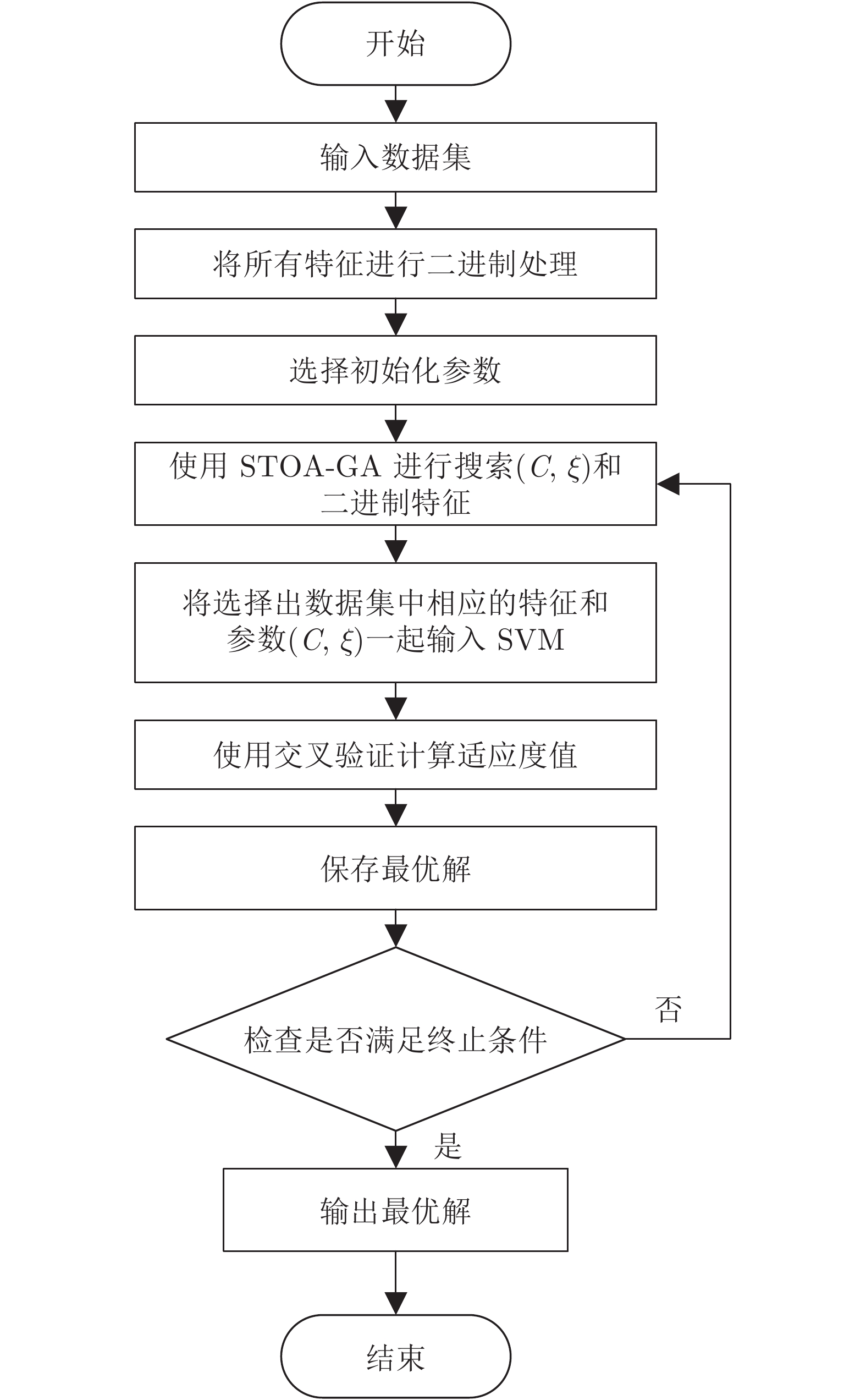
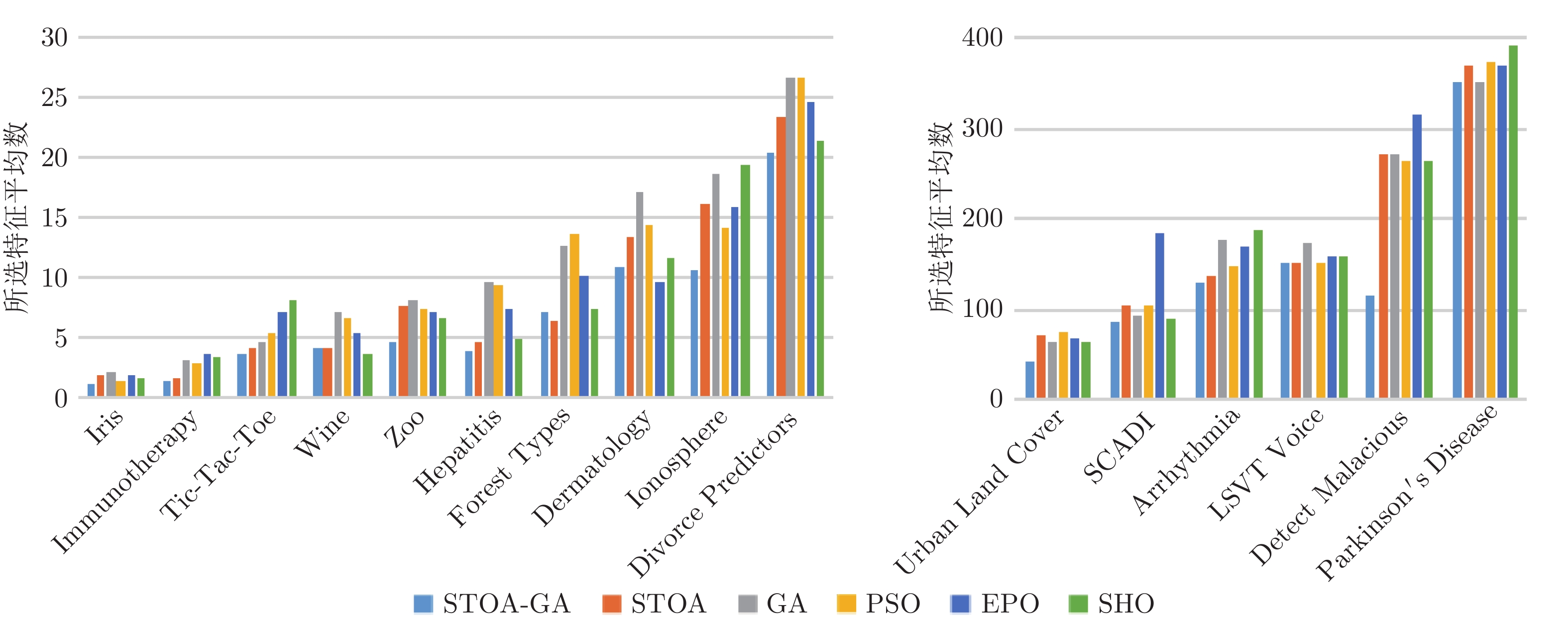
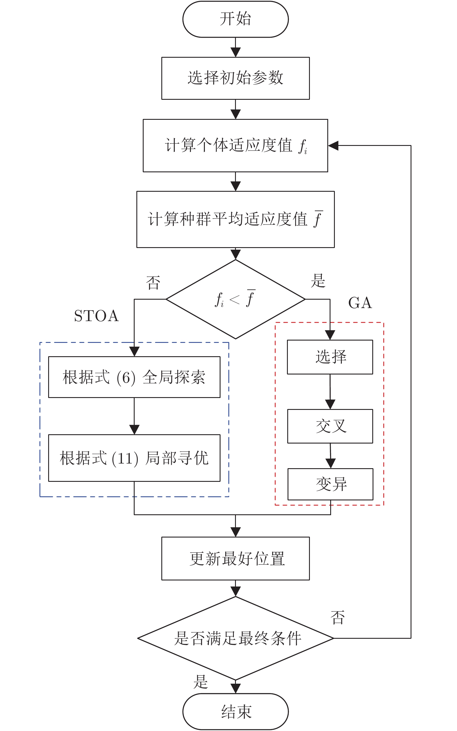
摘要: 针对传统支持向量机方法用于数据分类存在分类精度低的不足问题, 将支持向量机分类方法与特征选择同步结合, 并利用智能优化算法对算法参数进行优化研究. 首先将遗传算法(Genetic algorithm, GA)和乌燕鸥优化算法(Sooty tern optimization algorithm, STOA)进行混合, 先通过对平均适应度值进行评估, 当个体的适应度函数值小于平均值时采用遗传算法对其进行局部搜索的加强, 否则进行乌燕鸥本体优化过程, 同时将支持向量机内核函数和特征选择目标共同作为优化对象, 利用改进后的STOA-GA寻找最适应解, 获得所选的特征分类结果. 其次, 通过16组经典UCI数据集和实际乳腺癌数据集进行数据分类研究, 在最佳适应度值、所选特征个数、特异性、敏感性和算法耗时方面进行对比研究, 实验结果表明, 该算法可以更加准确地处理数据, 避免冗余特征干扰, 在数据挖掘领域具有更广阔的工程应用前景.Abstract: In view of the shortcomings of traditional support vector machine in data classification, this paper combines support vector machine classification with feature selection synchronously, and uses intelligent optimization algorithm to optimize algorithm parameters. Firstly, the genetic algorithm (GA) is mixed with the sooty tern optimization algorithm (STOA). In this paper, the average fitness value is evaluated first. When the fitness function value of the individual is less than the average value, the GA is used to deepen the local search. Otherwise, the optimization process of the STOA itself is carried out.The SVM kernel function and the feature selection target are taken as the optimization object. The improved STOA-GA is used to find the most suitable solution and get the selected feature classification results. Secondly, through the data classification research of sixteen groups of classic UCI data sets and real breast cancer data sets, the best fitness value, the number of selected features, specificity, sensitivity and algorithm time-consuming are compared. The experimental results show that the algorithm proposed in this paper can deal with data more accurately, avoid redundant feature interference, and have a broader work in the field of data mining application prospect of the project.
-
表 1 实验数据集
Table 1 The data sets used in the experiments
序号 数据集 特征数 样本数 类别数 1 Iris 4 150 3 2 Immunotherapy 8 90 2 3 Tic-Tac-Toe 9 958 2 4 Wine 13 178 3 5 Zoo 17 101 7 6 Hepatitis 19 155 2 7 Forest Types 27 326 4 8 Dermatology 33 366 6 9 Ionosphere 34 351 2 10 Divorce Predictors 54 170 2 11 Urban Land Cover 148 168 9 12 SCADI 206 70 7 13 Arrhythmia 279 452 16 14 LSVT Voice Rehabilitation 309 126 2 15 Detect Malacious Executable (AntiVirus) 513 373 2 16 Parkinson's Disease 754 756 2  下载: 导出CSV
表 2 对比算法的参数
Table 2 Parameters of the compared algorithms
算法 参数 设定值 STOA-GA 控制变量${C_f}$ 2 随机变量${C_B}$ [0, 0.5] 螺旋常数$u,v$ 1 交叉概率$Pc$ 0.95 变异概率$Pm$ 0.05 STOA[29] 控制变量${C_f}$ 2 随机变量${C_B}$ [0, 0.5] 螺旋常数$u,v$ 1 GA[32] 交叉概率$Pc$ 0.95 变异概率$Pm$ 0.05 PSO[15] 学习因子${c_1},{c_2}$ 1.5 权重因子$\omega $ 0.75 速度$v$ [0, 1] 常数${\rm{a}}$ 2 SHO[16] 控制因子$h$ [0, 5] 随机向量$M$ [0.5, 1] EPO[17] 移动参数$M$ 2 控制参数$f$ [2, 3] 控制参数$l$ [1.5, 2]
下载: 导出CSV
表 3 各算法运行时间平均值(s)
Table 3 The average time of each algorithm (s)
数据集 STOA-GA STOA GA PSO EPO SHO Iris 12.71 12.09 18.49 14.36 15.28 14.41 Immunotherapy 7.09 6.95 13.89 7.52 10.23 9.22 Tic-Tac-Toe 169.67 169.29 180.41 171.52 181.08 189.53 Wine 40.23 39.67 50.34 39.67 48.81 51.26 Zoo 16.95 16.25 19.96 16.49 20.38 19.45 Hepatitis 22.90 22.48 26.62 24.51 28.24 27.51 Forest Types 120.54 120.35 122.63 115.57 120.82 119.60 Dermatology 97.69 93.76 120.28 97.74 117.21 115.87 Ionosphere 74.74 71.91 84.92 85.09 86.96 81.92 Divorce Predictors 29.17 27.26 45.24 32.63 42.41 32.87 Urban Land Cover 186.15 185.79 186.19 188.76 192.15 207.50 SCADI 45.54 42.27 61.18 58.72 61.47 61.06 Arrhythmia 4132.40 4286.94 5382.19 4802.38 4582.08 5129.23 LSVT Voice 110.32 104.39 110.07 105.10 103.71 102.43 Detect Malacious 151.86 109.94 466.58 837.45 664.20 829.48 Parkinson's Disease 138.06 135.02 149.29 145.62 146.73 144.75
下载: 导出CSV
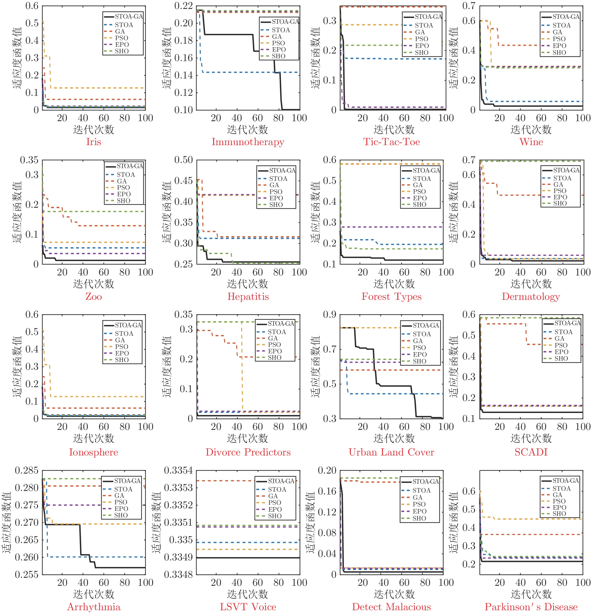
表 4 各算法适应度函数平均值
Table 4 The average fitness of each algorithm
数据集 STOA-GA STOA GA PSO EPO SHO Iris 0.0138 0.0231 0.0637 0.1294 0.0277 0.0202 Immunotherapy 0.101 0.1431 0.2125 0.2129 0.2163 0.2172 Tic-Tac-Toe 0.004 0.1731 0.3477 0.2305 0.0118 0.2164 Wine 0.0282 0.0593 0.4352 0.2945 0.2925 0.2849 Zoo 0.0131 0.0563 0.1292 0.0744 0.0351 0.1767 Hepatitis 0.2551 0.3123 0.4532 0.4156 0.4174 0.2549 Forest Types 0.1256 0.1953 0.5817 0.5841 0.2799 0.1742 Dermatology 0.0221 0.0384 0.4647 0.0367 0.0614 0.6913 Ionosphere 0.0334 0.0681 0.3547 0.3508 0.0505 0.3561 Divorce Predictors 0.0113 0.0226 0.2088 0.0262 0.0226 0.3269 Urban Land Cover 0.3012 0.4443 0.5807 0.8244 0.6257 0.6422 SCADI 0.1316 0.1607 0.4573 0.1607 0.1647 0.5844 Arrhythmia 0.2564 0.2603 0.2801 0.2699 0.2766 0.2823 LSVT Voice 0.3349 0.3350 0.3357 0.3349 0.3352 0.3352 Detect Malacious 0.0048 0.0104 0.1777 0.0129 0.0124 0.1855 Parkinson's Disease 0.2628 0.2838 0.3936 0.4676 0.2817 0.2872
下载: 导出CSV
表 5 各算法适应度函数标准差
Table 5 The standard deviation of fitness of each algorithm
数据集 STOA-GA STOA GA PSO EPO SHO Iris 0.0042 0.0067 0.0322 0.1 0.0067 0.0089 Immunotherapy 0.0206 0.1031 0.1821 0.2032 0.1988 0.0976 Tic-Tac-Toe 0.0067 0.0127 0.0148 0.0286 0.0174 0.0053 Wine 0.0101 0.0153 0.0218 0.0279 0.0101 0.0129 Zoo 0.0077 0.01 0.0272 0.0301 0.0089 0.0103 Hepatitis 0.0288 0.0429 0.2157 0.2891 0.1038 0.0302 Forest Types 0.0177 0.0282 0.0139 0 0.0234 0.0356 Dermatology 0.0133 0.0211 0.3036 0.0167 0.0314 0.3781 Ionosphere 0 0.0038 0.0287 0.0107 0.0183 0.0046 Divorce Predictors 0.0067 0.0133 0.1367 0.0083 0.0087 0.1492 Urban Land Cover 0.1044 0.1253 0.2517 0.1021 0.2089 0.2182 SCADI 0.0681 0.1372 0.1879 0.0706 0.1041 0.1645 Arrhythmia 0.1267 0.1146 0.1028 0.1382 0.1256 0.1474 LSVT Voice 0.0010 0 0.0012 0 0.0017 0.0039 Detect Malacious 0 0.0024 0.0147 0.0037 0 0.0183 Parkinson's Disease 0.0923 0.1032 0.1373 0.2104 0.1342 0.1567
下载: 导出CSV
表 6 各算法特异性(%)
Table 6 The specificity of each algorithm (%)
数据集 DT NB KNN SVM 本文方法 Ionosphere 89.64 79.67 96.03 93.84 97.67 Tic-Tac-Toe 90.56 84.32 99.43 98.54 100 Hepatitis 72.17 60.51 78.34 74.23 77.34 Immunotherapy 80.89 76.55 86.56 84.99 90.76 Divorce Predictors 91.32 85.33 98.76 93.67 100
下载: 导出CSV
表 8 各算法精确度(%)
Table 8 The accuracy of each algorithm (%)
数据集 DT NB KNN SVM 本文方法 Ionosphere 89.23 78.15 93.47 92.18 96.87 Tic-Tac-Toe 89.63 83.92 97.14 95.26 100 Hepatitis 72.04 57.43 77.54 72.31 75.19 Immunotherapy 79.65 74.69 85.71 82.97 90.00 Divorce Predictors 90.18 84.22 97.91 92.36 100
下载: 导出CSV
表 7 各算法敏感性(%)
Table 7 The sensitivity of each algorithm (%)
数据集 DT NB KNN SVM 本文方法 Ionosphere 88.67 76.37 91.78 90.13 95.48 Tic-Tac-Toe 87.13 83.67 95.43 93.27 99.54 Hepatitis 71.96 55.82 76.71 69.38 73.11 Immunotherapy 79.34 73.13 84.52 80.26 89.05 Divorce Predictors 89.03 84.01 95.39 91.67 98.75
下载: 导出CSV
表 9 乳腺癌数据集特征信息
Table 9 The breast cancer data set feature information
序号 英文简称 说明 1 Age 年龄, [10, 99]岁, 每10岁为1个区间, 共9个区间 2 Menopause 绝经期, 分为未绝经、40岁之后绝经、40岁之前绝经 3 Tumor-size 肿瘤大小, [0, 59]mm, 每5为1个区间, 共12个区间 4 Inv-nodes 淋巴结个数, [0, 39], 每3个为1个区间, 共13个区间 5 Node-caps 结节冒有无 6 Deg-malig 肿瘤恶性程度, 分为1、2、3三种, 3恶性程度最高 7 Breast 分为左和右两部分 8 Breast-quad 分为左上、左下、右上、右下4个区域 9 Irradiat 是否有放射性治疗经历
下载: 导出CSV
表 10 STOA-GA算法的10次实验运行结果
Table 10 The results of 10 experiments of STOA-GA
序号 分类准确
率 (%)选择特征
个数适应度值 时间 (s) 特异性
(%)敏感性
(%)1 97.62 5 0.0291 64.08 97.87 96.83 2 97.56 4 0.0286 63.83 97.75 96.12 3 96.74 5 0.0378 35.57 97.98 91.53 4 97.48 5 0.0305 64.15 98.64 96.05 5 98.21 4 0.0222 62.09 98.51 97.66 6 97.56 4 0.0286 60.49 97.87 96.83 7 97.66 5 0.0287 64.71 97.80 97.45 8 97.98 4 0.0244 62.01 98.03 97.89 9 96.28 5 0.0424 64.71 98.37 91.31 10 98.03 4 0.0239 68.29 98.37 97.76
下载: 导出CSV
表 11 10次实验均入选的特征
Table 11 The selected feature of 10 experiments
序号 特征 3 肿瘤大小 4 淋巴结个数 5 结节冒有无 6 肿瘤恶性程度
下载: 导出CSV
-
[1] 于洪, 何德牛, 王国胤, 李劼, 谢永芳. 大数据智能决策. 自动化学报, 2020, 46(5): 878-896YU Hong, HE De-Niu, WANG Guo-Yin, LI Jie, XIE Yong-Fang. Big Data for Intelligent Decision Making. Acta Automatica Sinica, 2020, 46(5): 878-896 [2] 贾涛, 韩萌, 王少峰, 杜诗语, 申明尧. 数据流决策树分类方法综述. 南京师大学报(自然科学版), 2019, 42(04): 49-60Jia Tao, Han Meng, Wang Shao-Feng, Du Shi-Yu, Shen Ming-Yao. Survey of decision tree classification methods over data streams. Journal of Nanjing Normal University (Natural Science Edition), 2019, 42(04): 49-60 [3] 崔良中, 郭福亮, 宋建新. 基于Map/Reduce的朴素贝叶斯数据分类算法研究. 海军工程大学学报, 2019, 31(04): 7-10 doi: 10.7495/j.issn.1009-3486.2019.04.002Cui Liang-Zhong, Guo Fu-Liang, Song Jian-Xin. Research on native Bayesian data classification algorithm based on Map/Reduce. Journal of Naval University of Engineering, 2019, 31(04): 7-10 doi: 10.7495/j.issn.1009-3486.2019.04.002 [4] 王景文, 李伟, 李永彬. 基于KNN的中医胃疼病患者分类研究 电脑与信息技术, 2019, 27(05): 40-43 doi: 10.3969/j.issn.1005-1228.2019.05.012Wang Jing-Wen, Li Wei, Li Yong-Bin. The research on classification of patients with stomachache in traditional Chinese medicine based on KNN. Computer and Information Technology, 2019, 27(05): 40-43 doi: 10.3969/j.issn.1005-1228.2019.05.012 [5] 丁世涛, 卢军, 洪鸿辉, 黄傲, 郭致远. 基于SVM的文本多选择分类系统的设计与实现. 计算机与数字工程, 2020, 48(01): 147-152 doi: 10.3969/j.issn.1672-9722.2020.01.027Ding Shi-Tao, Lu Jun, Hong Hong-Hui, Huang Ao, Guo Zhi-Yuan. Design and Implementation of Chinese web page multiple choice classification system based on support vector machine. Computer and Digital Engineering, 2020, 48(01): 147-152 doi: 10.3969/j.issn.1672-9722.2020.01.027 [6] Chapelle O, Vapnik V, Bousquet O, Mukherjee S. Choosing multiple parameters for support vector machines. Machine Learning, 2002, 46(1-3): 131-159 [7] 刘昌平, 范明钮, 王光卫, 马素丽. 基于梯度算法的支持向量机参数优化方法. 控制与决策. 2008, 23(11): 1291-1295 doi: 10.3321/j.issn:1001-0920.2008.11.019Liu Chang-Ping, Fan Ming-Yu, Wang Guang-Wei, Ma Su-Li. Optimizing parameters of support vector machine based on gradient algorithm. Contro l and Decision, 2008, 23(11): 1291-1295 doi: 10.3321/j.issn:1001-0920.2008.11.019 [8] 刘东平, 单甘霖, 张岐龙, 段修生. 基于改进遗传算法的支持向量机参数优化. 网络新媒体技术. 2010, 31(5): 11-15 doi: 10.3969/j.issn.2095-347X.2010.05.003Liu Dong-Ping, Shan Gan-Lin, Zhang Qi-Long, Duan Xiu-Sheng. Parameters optimization of support vector machine based on improved genetic algorithm. Microcomputer Applications, 2010, 31(5): 11-15 doi: 10.3969/j.issn.2095-347X.2010.05.003 [9] 王振武, 孙佳骏, 尹成峰. 改进粒子群算法优化的支持向量机及其应用. 哈尔滨工程大学学报, 2016, 37(12): 1728-1733Wang Zhen-Wu, Sun Jia-Jun, Yin Cheng-Feng. A support vector machine based on an improved particle swarm optimization algorithm and its application. Journal of Harbin Engineering University, 2016, 37(12): 1728-1733 [10] 石勇, 李佩佳, 汪华东. L2损失大规模线性非平行支持向量顺序回归模型. 自动化学报, 2019, 45(03): 505-517Shi Yong, Li Pei-Jia, Wang Hua-Dong. L2-loss large-scale linear nonparallel support vector ordinal regression. Acta Automatica Sinica, 2019, 45(03): 505-517 [11] Yu X, Chu Y, Jiang F, Guo Y, Gong D W. SVMs Classification Based Two-side Cross Domain Collaborative Filtering by inferring intrinsic user and item features. Knowledge-Based Systems, 2018, 141: 80-91 doi: 10.1016/j.knosys.2017.11.010 [12] Zhang Y, Gong D W, Cheng J. Multi-Objective Particle Swarm Optimization Approach for Cost-Based Feature Selection in Classification. IEEE/ACM Transactions on Computational Biology and Bioinformatics, 2017, 14(1): 64-75 doi: 10.1109/TCBB.2015.2476796 [13] Zhang Y, Song X F, Gong D W. A return-cost-based binary firefly algorithm for feature selection, Information Sciences, 2017, 418–419: 561-574 [14] 张文杰, 蒋烈辉. 一种基于遗传算法优化的大数据特征选择方法. 计算机应用研究, 2020, 37(01): 50-52+56Zhang Wen-Jie, Jiang Lie-Hui. Using genetic algorithm for feature selection optimization on big data processing. Application Research of Computers, 2020, 37(01): 50-52+56 [15] 李炜, 巢秀琴. 改进的粒子群算法优化的特征选择方法. 计算机科学与探索, 2019, 13(06): 990-1004Li Wei, Chao Xiu-Qin. Improved particle swarm optimization method for feature selection. Journal of Frontiers of Computer Science and Technology, 2019, 13(06): 990-1004 [16] Jia H M, Li J D, Song W L, Peng X X, Lang C B, Li Y. Spotted hyena optimization algorithm with simulated annealing for feature selection. IEEE ACCESS, 2019, 7: 71943-71962 doi: 10.1109/ACCESS.2019.2919991 [17] Baliarsingh S K, Ding W, Vipsita S, Bakshi S. A memetic algorithm using emperor penguin and social engineering optimization for medical data classification. Applied Soft Computing, 2019, 85: 1568-4946 [18] Zhang Y, Wang Q, Gong D W, Song X F. Nonnegative Laplacian embedding guided subspace learning for unsupervised feature selection. Pattern Recognition, 2019, 93: 337-352 doi: 10.1016/j.patcog.2019.04.020 [19] 齐子元, 房立清, 张英堂. 特征选择与支持向量机参数同步优化研究. 振动. 测试与诊断, 2010, 30(02): 111-114+205Qi Zi-Yuan, Fang Li-Qing, Zhang Ying-Tang, Synchro-Optimization of Feature Selection and Parameters of Support Vector Machine. Journal of Vibration, Measurement& Diagnosis, 2010, 30(02): 111-114+205 [20] 沈永良, 宋杰, 万志超. 基于改进烟花算法的SVM特征选择和参数优. 微电子学与计算机, 2018, 35(01): 21-25Shen Yong-Liang, Song Jie, Wan Zhi-Chao. Improved Fireworks Algorithm for Support Vector Machine Feature Selection and Parameters Optimization. Microelectronics & Computer, 2018, 35(01): 21-25 [21] Ibrahim A, Ala’ M A, Hossam F, Mohammad A H, Seyedali M, Heba S. Simultaneous feature selection and support vector machine optimization using the grasshopper optimization algorithm. Cognitive Computation, 2018, 10(3): 478-495 doi: 10.1007/s12559-017-9542-9 [22] 肖辉辉, 万常选, 段艳明, 谭黔林. 基于引力搜索机制的花朵授粉算法. 自动化学报, 2017, 43(4): 576-594Xiao Hui-Hui, Wan Chang-Xuan, Duan Yan-Ming, Tan Qian-Lin. Flower pollination algorithm based on gravity search mechanism. Acta Automatica Sinica, 2017, 43(4): 576-594 [23] Fraser A S. Simulation of Genetic Systems by Automatic Digital Computers Ⅱ. Effects of Linkage on Rates of Advance under Selection. Australian Journal of Biological Sciences, 1957, 10(4): 492-500 doi: 10.1071/BI9570492 [24] 马炫, 李星, 唐荣俊, 刘庆. 一种求解符号回归问题的粒子群优化算法. 自动化学报, 2020, 46(8): 1714-1726Ma Xuan, Li Xing, Tang Rong-Jun, Liu Qing. A particle swarm optimization approach for symbolic regression. Acta Automatica Sinica, 2020, 46(8): 1714-1726 [25] Mirjalili S, Lewis A. The whale optimization algorithm. Advances in Engineering Software, 2016, 95(1): 51-67 [26] Wolpert D H, Macready W G. No free lunch theorems for optimization. IEEE Trans on Evolutionary Computation, 1997, 1(1): 67-82 doi: 10.1109/4235.585893 [27] 唐晓娜, 张和生. 一种混合粒子群优化遗传算法的高分影像特征优化方法. 遥感信息, 2019, 34(06): 113-118 doi: 10.3969/j.issn.1000-3177.2019.06.018Tang Xiao-Na, Zhang He-Sheng. A hybrid particle swarm optimization genetic algorithm for high score image feature optimization. Remote Sensing Information, 2019, 34(06): 113-118 doi: 10.3969/j.issn.1000-3177.2019.06.018 [28] 卓雪雪, 苑红星, 朱苍璐, 钱鹏. 蚁群遗传混合算法在求解旅行商问题上的应用. 价值工程, 2020, 39(02): 188-193Zhuo Xue-Xue, Yuan Hong-Xing, Zhu Cang-Lu, Qian Peng. The application of ant colony and genetic hybrid algorithm on TSP. Value Engineering, 2020, 39(02): 188-193 [29] Dhiman G, Kaur A. STOA: A bio-inspired based optimization algorithm for industrial engineering problems. Engineering Applications of Artificial Intelligence, 2019, 82: 148-174 doi: 10.1016/j.engappai.2019.03.021 [30] Tamura K, Yasuda K. The Spiral Optimization Algorithm: Convergence Conditions and Settings. IEEE Transactions on Systems, Man & Cybernetics, 2017, 1−16 [31] Guo P, Wang X, Han Y. The enhanced genetic algorithms for the optimization design. In: Proceedings of the 2010 3rd International Conference on Biomedical Engineering and Informatics, Yantai, China: 2010. 2990−2994 [32] Junghans L, Darde N. Hybrid single objective genetic algorithm coupled with the simulated annealing optimization method for building optimization. Energy and Buildings, 2015, 86: 651-662 doi: 10.1016/j.enbuild.2014.10.039 [33] Jia H M, Li Y, Lang C B, Peng X X, Sun K J, Li J D. Hybrid grasshopper optimization algorithm and differential evolution for global optimization. Journal of Intelligent & Fuzzy Systems, 2019, 37(5): 1-12 [34] Cortes C, Vapnik V. Support-vector networks. Machine learning, 1995, 20: 273-297 [35] Cai Zhi-ling, Zhu W. Feature selection for multi-label classification using neighborhood preservation. IEEE/CAA Journal of Automatica Sinica, 2018, 5(1): 320-330 doi: 10.1109/JAS.2017.7510781 [36] Dash M, Liu H, Feature selection for classificarion. Intelligent Data Analysis, 1997, 1: 131-156. doi: 10.3233/IDA-1997-1302 [37] 孙亮, 韩崇昭, 沈建京, 戴宁. 集成特征选择的广义粗集方法与多分类器融合. 自动化学报, 2008, 34(3): 298-304Sun Liang, Han Chong-Zhao, Shen Jian-Jing, Dai Ning. Generalized rough set method for ensemble feature selection and multiple classifier fusion. Acta Automatica Sinica, 2008, 34(3): 298-304 [38] 林达坤, 黄世国, 林燕红, 洪铭淋. 基于差分进化和森林优化混合的特征选择. 小型微型计算机系统, 2019, 40(6): 1210-1214Lin Da-Kun, Huang Shi-Guo, Lin Yan-Hong, Hong Ming-Lin. Feature selection based on hybrid differential evolution and forest optimization. Journal of Chinese Computer Systems, 2019, 40(6): 1210-1214 [39] 丁胜, 张进, 李波. 改进的MEA进行特征选择及SVM参数同步优化. 计算机工程与应用, 2017, 53(08): 120-125+179Ding Sheng, Zhang Jin, Li Bo. Improved MEA for feature selection and SVM parameters optimization. Computer Engineering and Applications, 2017, 53(08): 120-125+179. [40] Blake C, UCI Repository of Machine Learning Databases. [Online], available: http://www.ics.uci.edu/?mlearn/MLRepository.html, July 5, 2020 [41] Emary E, Zawbaa H M, Hassanien A E. Binary ant lion approaches for feature selection, Neurocomputing, 2016, 213: 54-65 doi: 10.1016/j.neucom.2016.03.101 -

 下载:
下载:


计量
- 文章访问数: 2211
- HTML全文浏览量: 736
- PDF下载量: 241
- 被引次数: 0
