

-
摘要: 双目深度估计的在线适应是一个有挑战性的问题, 其要求模型能够在不断变化的目标场景中在线连续地自我调整并适应于当前环境. 为处理该问题, 提出一种新的在线元学习适应算法(Online meta-learning model with adaptation, OMLA), 其贡献主要体现在两方面: 首先引入在线特征对齐方法处理目标域和源域特征的分布偏差, 以减少数据域转移的影响; 然后利用在线元学习方法调整特征对齐过程和网络权重, 使模型实现快速收敛. 此外, 提出一种新的基于元学习的预训练方法, 以获得适用于在线学习场景的深度网络参数. 相关实验分析表明, OMLA和元学习预训练算法均能帮助模型快速适应于新场景, 在KITTI数据集上的实验对比表明, 本文方法的效果超越了当前最佳的在线适应算法, 接近甚至优于在目标域离线训练的理想模型.Abstract: This work tackles the problem of online adaptation for stereo depth estimation, that consists in continuously adapting a deep network to a target video recorded in an environment different from that of the source training set. To address this problem, we propose a novel online meta-learning model with adaptation (OMLA). Our proposal is based on two main contributions. First, to reduce the domain-shift between source and target feature distributions we introduce an online feature alignment procedure derived from batch normalization. Second, we devise a meta-learning approach that exploits feature alignment for faster convergence in an online learning setting. Additionally, we propose a meta-pre-training algorithm in order to obtain initial network weights on the source dataset which facilitate adaptation on future data streams. Experimentally, we show that both OMLA and meta-pre-training help the model to adapt faster to a new environment. Our proposal is evaluated on the KITTI dataset, where we show that our method outperforms both algorithms trained on the target data in an offline setting and state-of-the-art adaptation methods.
-
Key words:
- Depth estimation /
- online learning /
- meta-learning /
- domain adaptation /
- deep neural network
-
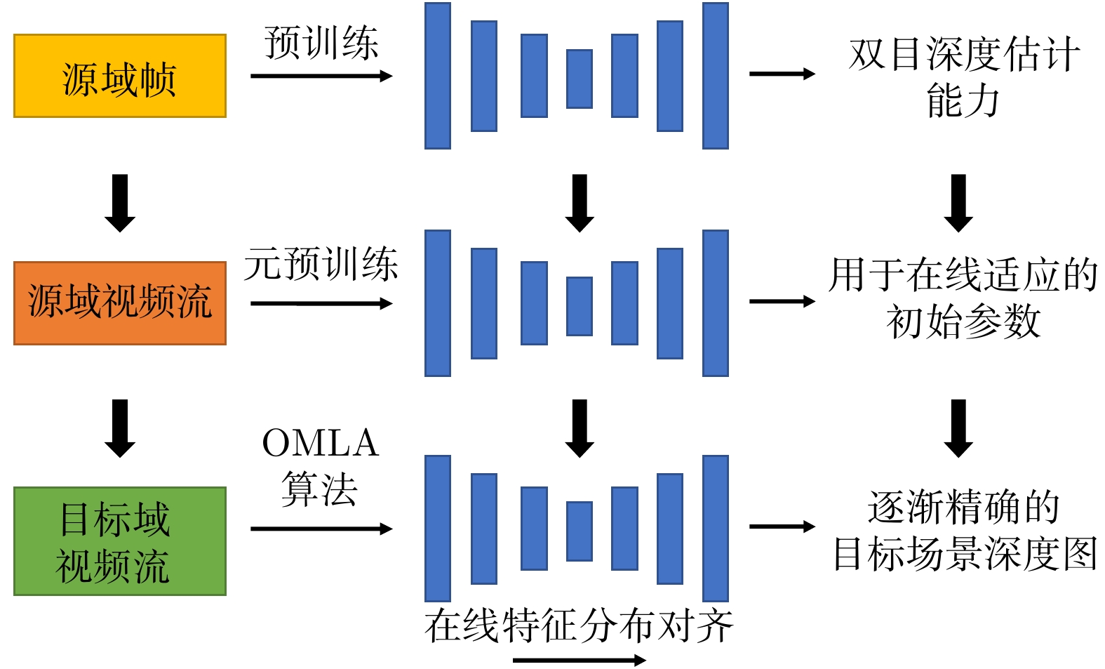
图 1 本文提出的基于元学习的深度估计在线适应算法框架
Fig. 1 The proposed meta-learning framework for online stereo adaptation
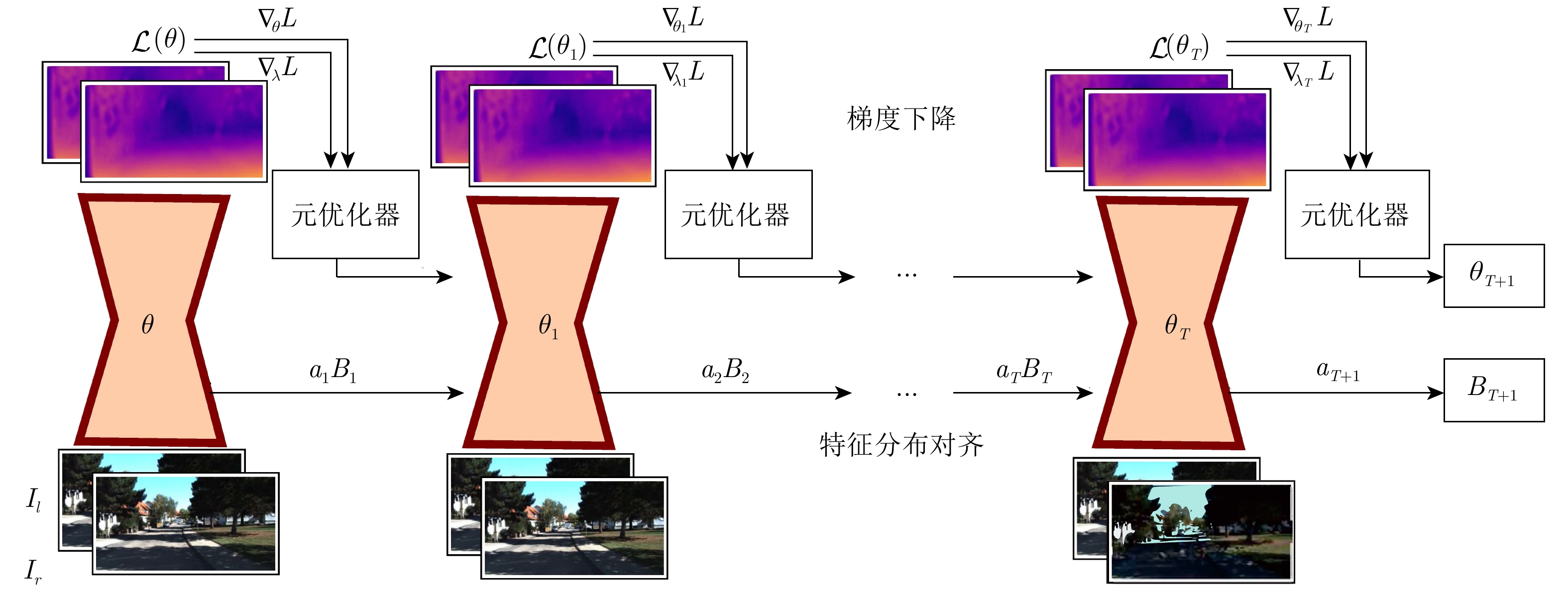
图 2 本文提出的在线元学习适应方法
Fig. 2 The proposed online meta-learning with adaptation (OMLA) method

图 3 在KITTI Eigen测试集中3个不同视频序列上的效果 (为了展示模型的在线适应效果随时间的变化, 此处展示了视频初始, 中段和末段时刻的深度估计效果)
Fig. 3 Performance on three different videos of KITTI Eigen test (We illustrated predictions of initial, medium, and last frames)
表 1 KITTI Eigen测试集的算法消融实验 (仅评估 50 m之内的深度估计效果)
Table 1 Ablation study on KITTI Eigen test set (the results are evaluated within 50 m)
方法 预训练方式 平均得分 最后 20% 帧的平均得分 RMSE Abs Rel Sq Rel ${\rm{RMSE} }_{ {\rm{log} } }$ RMSE Abs Rel Sq Rel ${\rm{RMSE} }_{ {\rm{log} } }$ 基准方法 无 12.2012 0.4357 5.5672 1.3598 12.2874 0.4452 5.5213 1.3426 基准方法 标准预训练方法 9.0518 0.2499 3.2901 0.9503 9.0309 0.2512 3.3104 0.9495 仅在线特征分布对齐 3.6135 0.1250 0.6972 0.2041 3.5857 0.1031 0.6887 0.1910 OMLA 算法 3.5027 0.0923 0.6611 0.1896 3.3986 0.0882 0.6579 0.1735 基准方法 元预训练方法 8.8230 0.2305 3.0578 0.9324 8.7061 0.2273 2.9804 0.9065 仅在线特征分布对齐 3.5043 0.0950 0.6627 0.1992 3.4831 0.0896 0.6545 0.1921 OMLA 算法 ${\bf{ {3.4051}}}$ ${\bf{ 0.0864}}$ ${\bf{{0.6256}}}$ ${\bf{ 0.1852}}$ ${\bf{ 3.3803 }}$ ${\bf{ 0.0798}}$ ${\bf{{0.6176}}}$ ${\bf{{0.1801}}}$  下载: 导出CSV
表 2 不同网络模型和数据库上的结果对比
Table 2 Comparison on different network architectures and datasets
网络模型 方法 预训练于 Synthia[20] 预训练于 Scene Flow Driving[41] 帧速率 (帧/s) RMSE Abs Rel Sq Rel ${\rm{RMSE} }_{ {\rm{log} } }$ RMSE Abs Rel Sq Rel ${\rm{RMSE} }_{ {\rm{log} } }$ ResNet[9] 基准方法 9.0518 0.2499 3.2901 0.8577 9.0893 0.2602 3.3896 0.8901 ${\bf{ 5.06}}$ OMLA + 元预训练 ${\bf{ 3.4051}}$ ${\bf{ 0.0864}}$ ${{\bf{{0.6256}}}}$ ${\bf{ 0.1852}}$ ${\bf{ 4.0573}}$ ${\bf{ 0.1231}}$ ${\bf{ 1.1532}}$ ${\bf{ 0.1985}}$ 3.40 MADNet[15] 基准方法 8.8650 0.2684 3.1503 0.8233 8.9823 0.2790 3.3021 0.8350 ${\bf{ 12.05}}$ OMLA + 元预训练 ${\bf{ 4.0236}}$ ${\bf{ 0.1756}}$ ${\bf{ 1.1825}}$ ${\bf{ 0.2501}}$ ${\bf{ 4.2179}}$ ${\bf{ 0.1883}}$ ${\bf{ 1.2761}}$ ${\bf{ 0.2523}}$ 9.56 DispNet[41] 基准方法 9.0222 0.2710 4.3281 0.9452 9.1587 0.2805 4.3590 0.9528 ${\bf{ 5.42}}$ OMLA + 元预训练 ${\bf{ 4.5201}}$ ${\bf{ 0.2396}}$ ${\bf{ 1.3104}}$ ${\bf{ 0.2503}}$ ${\bf{ 4.6314}}$ ${\bf{ 0.2457}}$ ${\bf{ 1.3541}}$ ${\bf{ 0.2516}}$ 4.00
下载: 导出CSV
表 3 与理想模型和当前最优方法的比较 (仅比较实际深度值小于50 m的像素点)
Table 3 Comparison with ideal models and state-of-the-art method (Results are only evaluated within 50 m)
网络模型 在线适应算法 预训练域 RMSE Abs Rel Sq Rel ${\rm{RMSE}}_{{\rm{log}}}$ $\alpha>1.25$ $\alpha>1.25^2$ $\alpha>1.25^3$ ResNet[9] 无 目标域 3.6975 0.0983 1.1720 0.1923 0.9166 0.9580 0.9778 基准方法 目标域 3.4359 ${\bf{ 0.0850}}$ 0.6547 0.1856 ${{\bf{{0.9203}}}}$ 0.9612 0.9886 L2A[35] 源域 3.5030 0.0913 0.6522 ${\bf{ 0.1840}}$ 0.9170 0.9611 0.9882 OMLA+元预训练 源域 ${\bf{ 3.4051}}$ 0.0864 ${\bf{ 0.6256 }}$ 0.1852 0.9170 ${\bf{ 0.9623}}$ ${\bf{ 0.9901}}$ MADNet[15] 无 目标域 ${{\bf{{3.8965}}}}$ 0.1793 1.2369 ${{\bf{{0.2457}}}}$ 0.9147 0.9601 0.9790 基准方法 目标域 3.9023 0.1760 1.1902 0.2469 ${\bf{ 0.9233}}$ 0.9652 0.9813 L2A[35] 源域 4.1506 0.1788 1.1935 0.2533 0.9131 0.9443 0.9786 OMLA+元预训练 源域 4.0236 ${{\bf{{0.1756}}}}$ ${{\bf{{1.1825}}}}$ 0.2501 0.9022 ${\bf{ 0.9658}}$ ${\bf{ 0.9842}}$ DispNet[41] 无 目标域 4.5210 0.2433 ${{\bf{{1.2801}}}}$ ${{\bf{{0.2490}}}}$ 0.9126 0.9472 ${{\bf{{0.9730}}}}$ 基准方法 目标域 4.5327 ${\bf{ 0.2368}}$ 1.2853 0.2506 ${\bf{ 0.9178}}$ ${\bf{ 0.9600}}$ 0.9725 L2A[35] 源域 4.6217 0.2410 1.2902 0.2593 0.9062 0.9513 0.9688 OMLA+元预训练 源域 ${{\bf{{4.5201}}}}$ 0.2396 1.3104 0.2503 0.9085 0.9460 0.9613
下载: 导出CSV
-
[1] Eigen D, Fergus R. Predicting depth, surface normals and semantic labels with a common multi-scale convolutional architecture. In: Proceedings of the IEEE International Conference on Computer Vision (ICCV). Santiago, Chile: IEEE, 2015. 2650−2658 [2] Laina I, Rupprecht C, Belagiannis V, Tombari F, Navab N. Deeper depth prediction with fully convolutional residual networks. In: Proceedings of the 4th International Conference on 3D Vision (3DV). Stanford, USA: IEEE, 2016. 239−248 [3] Fu H, Gong M M, Wang C H, Batmanghelich K, Tao D C. Deep ordinal regression network for monocular depth estimation. In: Proceedings of the IEEE/CVF Conference on Computer Vision and Pattern Recognition. Salt Lake City, USA: IEEE, 2018. 2002−2011 [4] Xu D, Wang W, Tang H, Liu H, Sebe N, Ricci E. Structured attention guided convolutional neural fields for monocular depth estimation. In: Proceedings of the IEEE/CVF Conference on Computer Vision and Pattern Recognition. Salt Lake City, USA: IEEE, 2018. 3917−3925 [5] Zhang Z Y, Cui Z, Xu C Y, Jie Z Q, Li X, Yang J. Joint task-recursive learning for semantic segmentation and depth estimation. In: Proceedings of the 15th European Conference on Computer Vision. Munich, Germany: Springer, 2018. 235−251 [6] Wofk D, Ma F C, Yang T J, Karaman S, Sze V. FastDepth: Fast monocular depth estimation on embedded systems. In: Proceedings of the International Conference on Robotics and Automation (ICRA). Montreal, Canada: IEEE, 2019. 6101−6108 [7] Ma F C, Karaman S. Sparse-to-dense: Depth prediction from sparse depth samples and a single image. In: Proceedings of the IEEE International Conference on Robotics and Automation (ICRA). Brisbane, Australia: IEEE, 2018. 1−8 [8] Garg R, Kumar B G V, Carneiro G, Reid I. Unsupervised CNN for single view depth estimation: Geometry to the rescue. In: Proceedings of the 14th European Conference on Computer Vision. Amsterdam, the Netherlands: Springer, 2016. 740−756 [9] Godard C, Aodha O M, Brostow G J. Unsupervised monocular depth estimation with left-right consistency. In: Proceedings of the IEEE Conference on Computer Vision and Pattern Recognition (CVPR). Honolulu, USA: IEEE, 2017. 270−279 [10] Pilzer A, Xu D, Puscas M, Ricci E, Sebe N. Unsupervised adversarial depth estimation using cycled generative networks. In: Proceedings of the International Conference on 3D Vision (3DV). Verona, Italy: IEEE, 2018. 587−595 [11] Pillai S, Ambruş R, Gaidon A. SuperDepth: Self-supervised, super-resolved monocular depth estimation. In: Proceedings of the International Conference on Robotics and Automation (ICRA). Montreal, Canada: IEEE, 2019. 9250−9256 [12] Mancini M, Karaoguz H, Ricci E, Jensfelt P, Caputo B. Kitting in the wild through online domain adaptation. In: Proceedings of the IEEE/RSJ International Conference on Intelligent Robots and Systems (IROS). Madrid, Spain: IEEE, 2018. 1103−1109 [13] Carlucci F M, Porzi L, Caputo B, Ricci E, Bulò S R. AutoDIAL: Automatic domain alignment layers. In: Proceedings of the IEEE International Conference on Computer Vision (ICCV). Venice, Italy: IEEE, 2017. 5077−5085 [14] Menze M, Geiger A. Object scene flow for autonomous vehicles. In: Proceedings of the IEEE Conference on Computer Vision and Pattern Recognition (CVPR). Boston, USA: IEEE, 2015. 3061−3070 [15] Tonioni A, Tosi F, Poggi M, Mattoccia S, Di Stefano L. Real-time self-adaptive deep stereo. In: Proceedings of the IEEE/CVF Conference on Computer Vision and Pattern Recognition (CVPR). Long Beach, USA: IEEE, 2019. 195−204 [16] Liu F Y, Shen C H, Lin G S, Reid I. Learning depth from single monocular images using deep convolutional neural fields. IEEE Transactions on Pattern Analysis and Machine Intelligence, 2016, 38(10): 2024-2039 doi: 10.1109/TPAMI.2015.2505283 [17] Yang N, Wang R, Stückler J, Cremers D. Deep virtual stereo odometry: Leveraging deep depth prediction for monocular direct sparse odometry. In: Proceedings of the 15th European Conference on Computer Vision. Munich, Germany: Springer, 2018. 835−852 [18] Silberman N, Hoiem D, Kohli P, Fergus R. Indoor segmentation and support inference from RGBD images. In: Proceedings of the 12th European Conference on Computer Vision. Florence, Italy: Springer, 2012. 746−760 [19] Geiger A, Lenz P, Urtasun R. Are we ready for autonomous driving? The KITTI vision benchmark suite. In: Proceedings of the IEEE Conference on Computer Vision and Pattern Recognition. Providence, USA: IEEE, 2012. 3354−3361 [20] Ros G, Sellart L, Materzynska J, Vazquez D, Lopez A M. The SYNTHIA dataset: A large collection of synthetic images for semantic segmentation of urban scenes. In: Proceedings of the IEEE Conference on Computer Vision and Pattern Recognition (CVPR). Las Vegas, USA: IEEE, 2016. 3234−3243 [21] Zhou T H, Brown M, Snavely N, Lowe D G. Unsupervised learning of depth and ego-motion from video. In: Proceedings of the IEEE Conference on Computer Vision and Pattern Recognition (CVPR). Honolulu, USA: IEEE, 2017. 1851−1858 [22] Kundu J N, Uppala P K, Pahuja A, Babu R V. AdaDepth: Unsupervised content congruent adaptation for depth estimation. In: Proceedings of the IEEE/CVF Conference on Computer Vision and Pattern Recognition. Salt Lake City, USA: IEEE, 2018. 2656−2665 [23] Csurka G. Domain adaptation for visual applications: A comprehensive survey. arXiv preprint arXiv: 1702.05374, 2017. [24] Long M S, Zhu H, Wang J M, Jordan M I. Deep transfer learning with joint adaptation networks. In: Proceedings of the 34th International Conference on Machine Learning. Sydney, Australia: JMLR.org, 2017. 2208−2217 [25] Venkateswara H, Eusebio J, Chakraborty S, Panchanathan S. Deep hashing network for unsupervised domain adaptation. In: Proceedings of the IEEE Conference on Computer Vision and Pattern Recognition (CVPR). Honolulu, USA: IEEE, 2017. 5018−5027 [26] Bousmalis K, Irpan A, Wohlhart P, Bai Y F, Kelcey M, Kalakrishnan M, et al. Using simulation and domain adaptation to improve efficiency of deep robotic grasping. In: Proceedings of the IEEE International Conference on Robotics and Automation (ICRA). Brisbane, Australia: IEEE, 2018. 4243−4250 [27] Sankaranarayanan S, Balaji Y, Castillo C D, Chellappa R. Generate to adapt: Aligning domains using generative adversarial networks. In: Proceedings of the IEEE/CVF Conference on Computer Vision and Pattern Recognition. Salt Lake City, USA: IEEE, 2018. 8503−8512 [28] Wulfmeier M, Bewley A, Posner I. Incremental adversarial domain adaptation for continually changing environments. In: Proceedings of the IEEE International Conference on Robotics and Automation (ICRA). Brisbane, Australia: IEEE, 2018. 1−9 [29] Li Y H, Wang N Y, Shi J P, Liu J Y, Hou X D. Revisiting batch normalization for practical domain adaptation. In: Proceedings of the 5th International Conference on Learning Representations. Toulon, France: OpenReview.net, 2017. [30] Mancini M, Porzi L, Bulò S R, Caputo B, Ricci E. Boosting domain adaptation by discovering latent domains. In: Proceedings of the IEEE/CVF Conference on Computer Vision and Pattern Recognition. Salt Lake City, USA: IEEE, 2018. 3771−3780 [31] Tobin J, Fong R, Ray A, Schneider J, Zaremba W, Abbeel P. Domain randomization for transferring deep neural networks from simulation to the real world. In: Proceedings of the IEEE/RSJ International Conference on Intelligent Robots and Systems. Vancouver, Canada: IEEE, 2017. 23−30 [32] Tonioni A, Poggi M, Mattoccia S, Di Stefano L. Unsupervised adaptation for deep stereo. In: Proceedings of the IEEE International Conference on Computer Vision (ICCV). Venice, Italy: IEEE, 2017. 1605−1613 [33] Pang J H, Sun W X, Yang C X, Ren J, Xiao R C, Zeng J, et al. Zoom and learn: Generalizing deep stereo matching to novel domains. In: Proceedings of the IEEE/CVF Conference on Computer Vision and Pattern Recognition. Salt Lake City, USA: IEEE, 2018. 2070−2079 [34] Zhao S S, Fu H, Gong M M, Tao D C. Geometry-aware symmetric domain adaptation for monocular depth estimation. In: Proceedings of the IEEE/CVF Conference on Computer Vision and Pattern Recognition (CVPR). Long Beach, USA: IEEE, 2019. 9788−9798 [35] Tonioni A, Rahnama O, Joy T, Di Stefano L, Ajanthan T, Torr P H S. Learning to adapt for stereo. In: Proceedings of the IEEE/CVF Conference on Computer Vision and Pattern Recognition (CVPR). Long Beach, USA: IEEE, 2019. 9661−9670 [36] Vinyals O, Blundell C, Lillicrap T, Kavukcuoglu K, Wierstra D. Matching networks for one shot learning. In: Proceedings of the 30th International Conference on Neural Information Processing Systems. Barcelona, Spain: Curran Associates Inc., 2016. 3637−3645 [37] Finn C, Abbeel P, Levine S. Model-agnostic meta-learning for fast adaptation of deep networks. In: Proceedings of the 34th International Conference on Machine Learning. Sydney, Australia: JMLR.org, 2017. 1126−1135 [38] Guo Y H, Shi H H, Kumar A, Grauman K, Rosing T, Feris R. SpotTune: Transfer learning through adaptive fine-tuning. In: Proceedings of the IEEE/CVF Conference on Computer Vision and Pattern Recognition (CVPR). Long Beach, USA: IEEE, 2019. 4805−4814 [39] Park E, Berg A C. Meta-tracker: Fast and robust online adaptation for visual object trackers. In: Proceedings of the 15th European Conference on Computer Vision. Munich, Germany: Springer, 2018. 587−604 [40] Wang P, Shen X H, Lin Z, Cohen S, Price B, Yuille A. Towards unified depth and semantic prediction from a single image. In: Proceedings of the IEEE Conference on Computer Vision and Pattern Recognition (CVPR). Boston, USA: IEEE, 2015. 2800−2809 [41] Mayer N, Ilg E, Häusser P, Fischer P, Cremers D, Dosovitskiy A, et al. A large dataset to train convolutional networks for disparity, optical flow, and scene flow estimation. In: Proceedings of the IEEE Conference on Computer Vision and Pattern Recognition (CVPR). Las Vegas, USA: IEEE, 2016. 4040−4048 [42] Paszke A, Gross S, Chintala S, Chanan G, Yang E, DeVito Z, et al. Automatic differentiation in PyTorch. In: Proceedings of the 31st Conference on Neural Information Processing Systems. Long Beach, USA: 2017. [43] Ioffe S, Szegedy C. Batch normalization: Accelerating deep network training by reducing internal covariate shift. In: Proceedings of the 32nd International Conference on International Conference on Machine Learning. Lille, France: JMLR.org, 2015. 448−456 [44] Kingma D P, Ba J. Adam: A method for stochastic optimization. In: Proceedings of the 3rd International Conference on Learning Representations. San Diego, USA: 2015. -

 下载:
下载:

计量
- 文章访问数: 1833
- HTML全文浏览量: 709
- PDF下载量: 255
- 被引次数: 0
