

Multi-scale Quantum Harmonic Oscillator Algorithm Based on Subpopulation Number Adaptive
-
摘要: 优化算法中多种群采样方式可转化为蒙特卡洛对当前函数积分的评估, 针对不同子种群对整体评估的差异性, 提出子种群规模 (个体数) 自适应的改进策略, 并用于多尺度量子谐振子优化算法(Multi-scale quantum harmonic oscillator algorithm, MQHOA) 的改进, 同时阐述多种群策略所具有的量子特性以及量子隧道效应与寻优性能的相关性. 已有的优化算法忽视了动态调节子种群规模对寻优能力的影响, 该策略通过动态调节子种群规模, 提高适应度差的子种群发生量子隧道效应的概率, 增强了算法的寻优能力. 将改进后的算法MQHOA-d (Multi-scale quantum harmonic oscillator algorithm based on dynamic subpopulation) 与 MQHOA 及其他优化算法在 CEC2013 测试集上进行测试, 结果表明原算法 MQHOA“早熟”问题在 MQHOA-d 中得到解决, 且 MQHOA-d 对多峰函数和复合函数优化具有显著优势, 求解误差和计算时间均小于几种经典优化算法.Abstract: The optimization algorithm of multiple subpopulations of sampling can be converted Monte Carlo evaluation function definite integral, because of the differences between different subpopulations in the overall evaluation, an adaptive strategy of subpopulation size (number of individuals) is proposed, which is used to improve multi-scale quantum harmonic oscillator optimization algorithm (MQHOA). The quantum properties of multi-population strategy and the correlation between quantum tunneling effect and optimization performance are discussed. The performance of existing optimization algorithm ignores the dynamic adjustment of subpopulation size influence on optimization ability, this strategy by dynamically adjusting population size, improve fitness poor child population incidence of quantum tunnel effect, increase the optimization ability of the algorithm. Compared the improved algorithm multi-scale quantum harmonic oscillator algorithm based on dynamic subpopulation (MQHOA-d) with MQHOA and other optimization algorithms on CEC2013 standard test functions. The experimental results show that the improved algorithm is more efficient in the optimization of basic multimodal functions and composition functions and the experimental results are better than several classical optimization algorithms and premature convergence problem has been solved.
-
Key words:
- Optimization algorithm /
- quantum tunneling effect /
- dynamic population /
- multi-populations /
- Monte Carlo
-
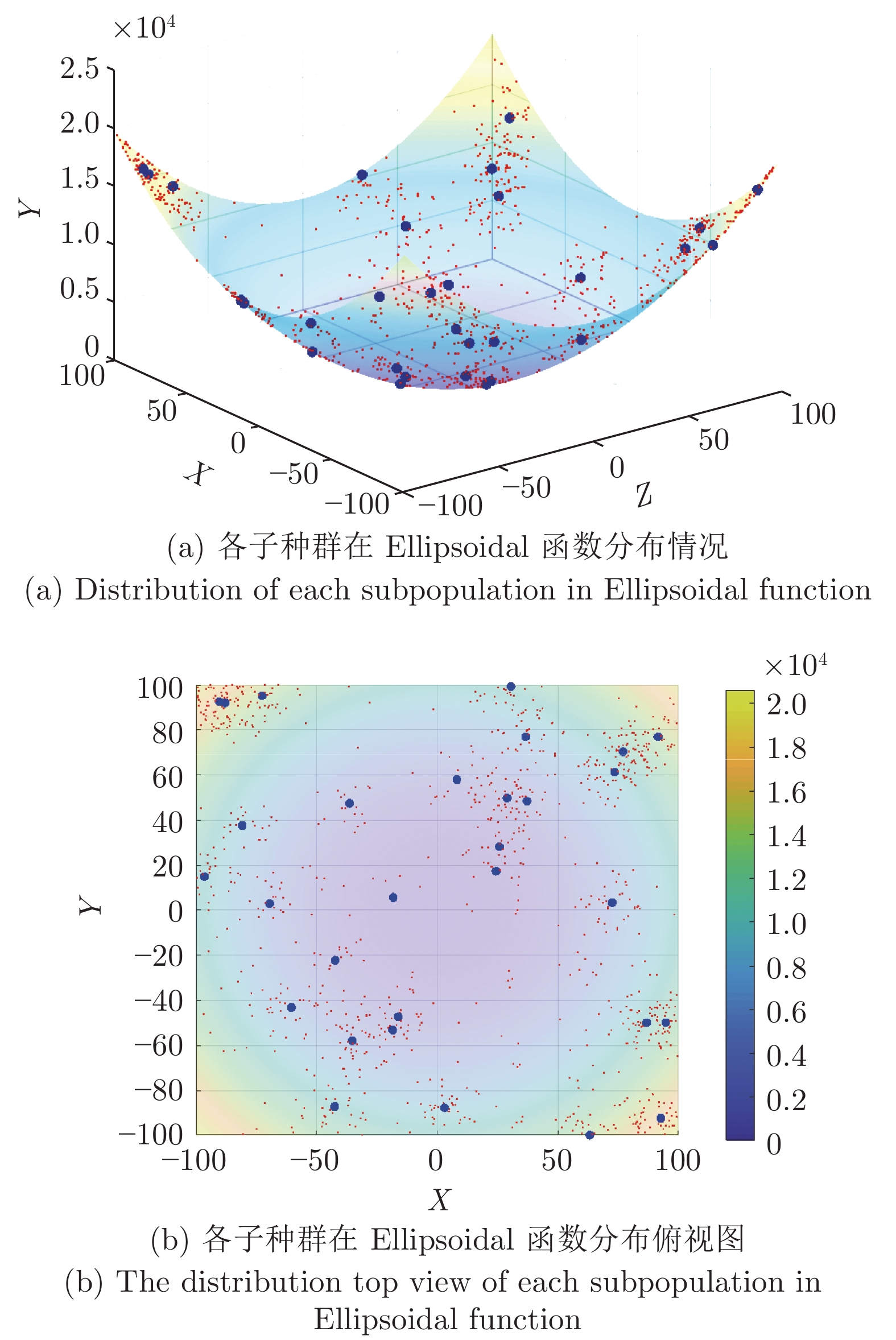
图 2 MQHOA-d所生成种群在Ellipsoidal函数二维空间分布示意图
Fig. 2 Schematic diagram of spatial distribution of subpopulations generated by MQHOA-d in Ellipsoidal function of 2D
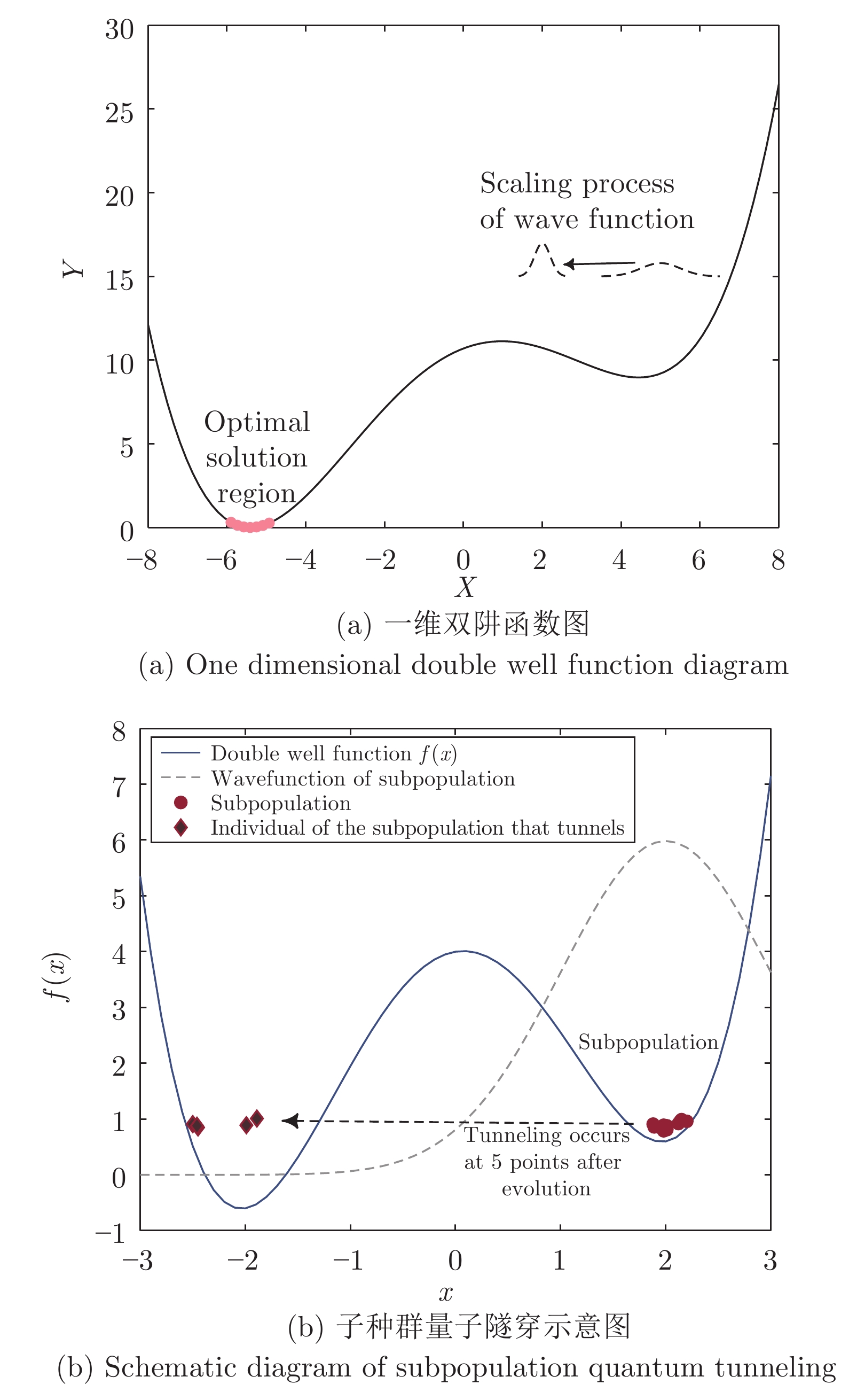
图 3 一维双阱函数图与隧道效应示意图
Fig. 3 One dimensional double well function diagram and tunnel effect diagram

图 4 MQHOA-d与MQHOA发生隧道效应点数量与迭代次数关系图
Fig. 4 The relationship between the number of tunneling points and the number of iterations between MQHOA-d and MQHOA
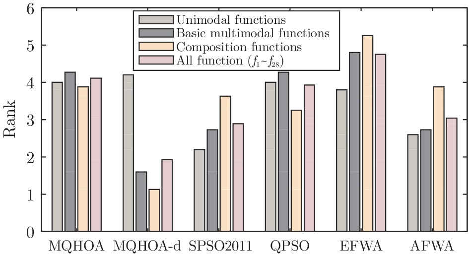
图 5 CEC2013测试集上各算法误差等级图(维度为30, 重复51次)
Fig. 5 Rank sum test results of all algorithms on CEC2013 test set (repeated 51 times in the 30-dimensional case)
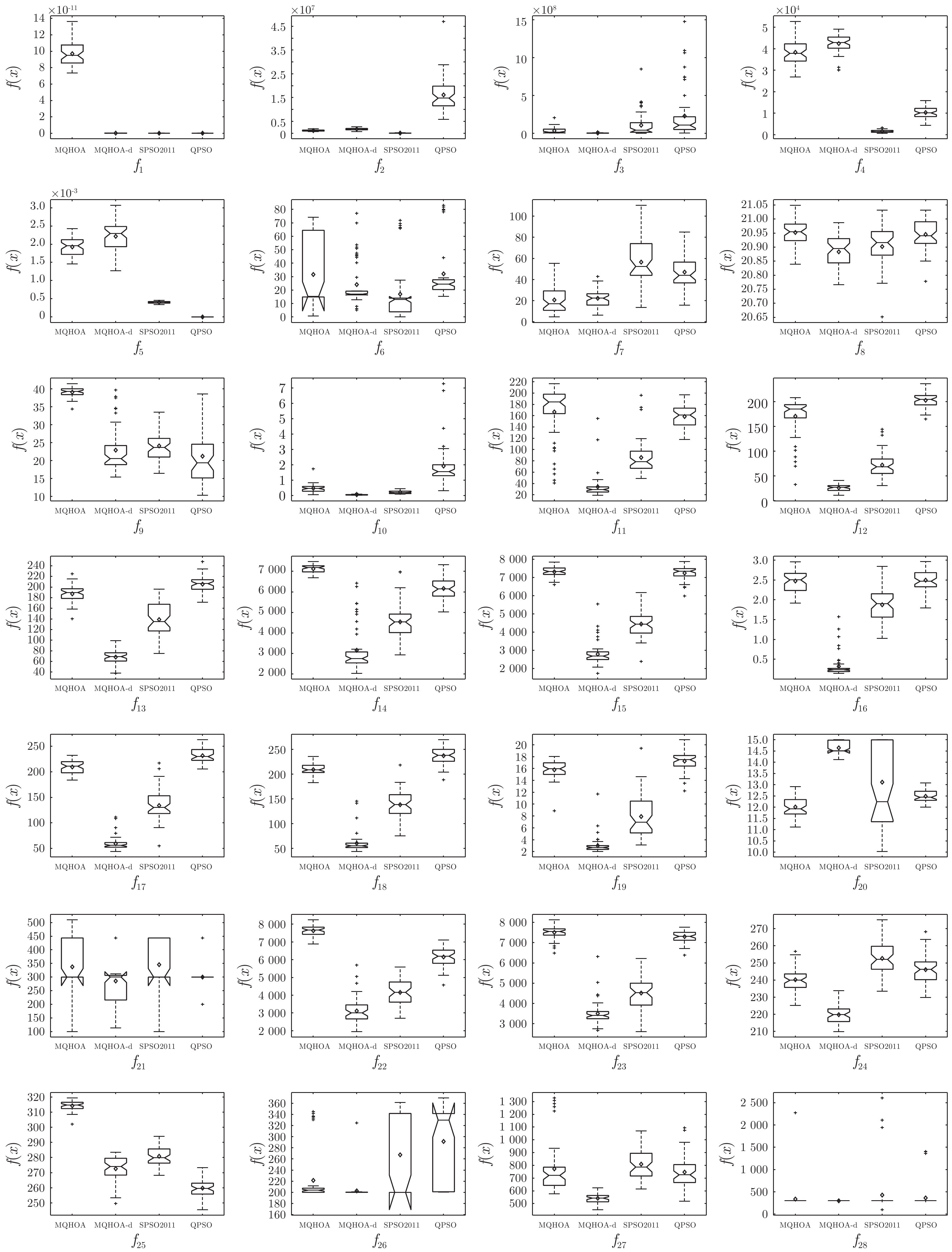
图 6 CEC2013测试函数在30维情况下重复51次实验箱体图
Fig. 6 Boxplots of CEC2013 benchmark functions repeated 51 times in the 30-dimensional case
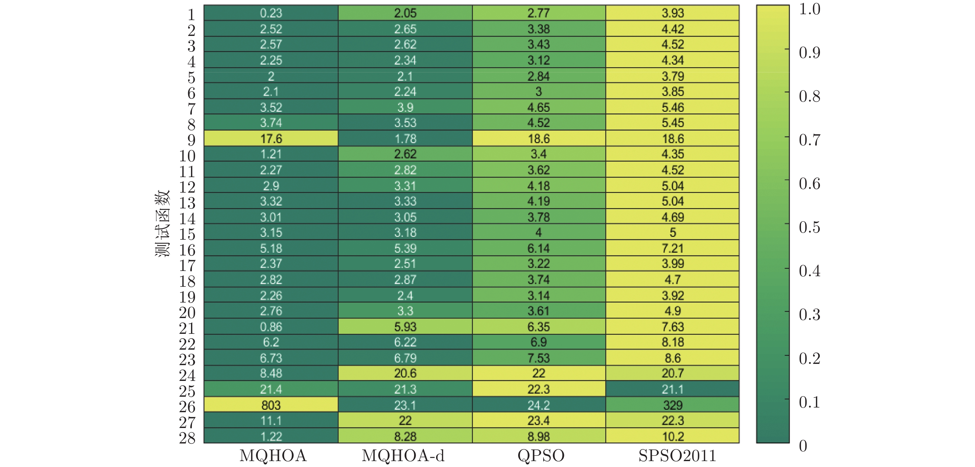
图 7 CEC2013测试函数在30维情况下各算法重复51次实验平均时间消耗热力图
Fig. 7 Rank of mean time consumption on CEC2013 repeated 51 times in the 30-dimensional case
表 1 量子理论与优化算法的对应关系
Table 1 The relationship between quantum theory and optimization algorithm
量子理论 优化算法 说明 势能评估/势能最低点 $f(x)/f(x)$ 的全局最小值 量子系统下将函数优化问题转化为寻找势能最低点问题 波函数 解的概率分布 量子系统下波函数对优化问题的概率描述 势阱等效 优化问题目标函数的近似方法 如QPSO中用Delta势阱逼近目标函数, MQHOA以谐振子逼近目标函数 势垒宽度 子种群位置到最优解的相对距离 势垒宽度越大, 隧道效应概率越低 量子隧道效应 跳出局部最优能力 波函数计算隧道效应概率, 增加迭代过程中发生隧道效应的采样点数量, 可提高算法性能  下载: 导出CSV
表 2 CEC2013测试函数维度为30情况下各算法51次重复实验的平均误差和标准差
Table 2 Mean errors and standard deviation of each algorithm on CEC2013 repeated 51 times in the 30-dimensional
$ f $ MQHOA MQHOA-d SPSO2011 QPSO EFWA AFWA MeanErr Std MeanErr Std MeanErr Std MeanErr Std MeanErr Std MeanErr Std 1 $9.71\times 10^{-11}$ $1.44\times 10^{-11}$ $3.25\times10^{-13}$ $1.14\times 10^{-13}$ $2.36\times 10^{-13}$ $4.46\times 10^{-14}$ $2.59\times 10^{-13}$ $9.12\times 10^{-14}$ $7.82\times 10^{-2}$ $1.31\times 10^{-2}$ ${{{\boldsymbol{0.00}}{\boldsymbol{\times}} {\boldsymbol{10}}^{{\boldsymbol{0}}} } }$ ${{{\boldsymbol{0.00}}{\boldsymbol{\times}}{\boldsymbol{10}}^{{\boldsymbol{0}}} } }$ 2 $1.15\times 10^{6}$ $2.65\times 10^{5}$ $1.76\times 10^{6}$ $3.97\times 10^{5}$ ${{{\boldsymbol{9.68}}{\boldsymbol{\times}} {\boldsymbol{10}}^{{\boldsymbol{4}}} } }$ ${{{\boldsymbol{4.82}}\times {\boldsymbol{10}}^{{\boldsymbol{4}}} } }$ $1.62\times 10^{7}$ $7.01\times 10^{6}$ $5.43\times 10^{5}$ $2.04\times 10^{5}$ $8.92\times 10^{5}$ $3.92\times 10^{5}$ 3 $3.32\times 10^{7}$ $ 3.94\times 10^{7} $ ${{{\boldsymbol{3.60}}\times {\boldsymbol{10}}^{{\boldsymbol{6}}} } }$ ${{{\boldsymbol{4.19}}\times {\boldsymbol{10}}^{{\boldsymbol{6}}} } }$ $ 1.07\times 10^{8} $ $ 1.58\times 10^{8} $ $ 2.28\times 10^{8} $ $ 3.23\times 10^{8} $ $ 1.26\times 10^{8} $ $ 2.15\times 10^{8} $ $ 1.26\times 10^{8} $ $ 1.54\times 10^{8} $ 4 $ 3.83\times 10^{4} $ $ 5.80\times 10^{3} $ $ 4.24\times 10^{4} $ $ 4.43\times 10^{3} $ $ 1.55\times 10^{3} $ $ 5.87\times 10^{2} $ $ 1.03\times 10^{4} $ $ 2.49\times 10^{3} $ ${{{\boldsymbol{1.09}}{\boldsymbol{\times}} {\boldsymbol{10^{0}}}}} $ ${{{\boldsymbol{3.53}}{\boldsymbol{\times}} {\boldsymbol{10}}^{{\boldsymbol{-}}{\boldsymbol{1}}} } }$ $ 1.14\times 10^{1} $ $ 6.83\times 10^{0} $ 5 $ 1.92\times 10^{-3} $ $ 2.46\times 10^{-4} $ $ 2.22\times 10^{-3} $ $ 4.23\times 10^{-4} $ $ 4.03\times 10^{-4} $ $ 2.92\times 10^{-5} $ ${{{\boldsymbol{3.40}}{\boldsymbol{\times}} {\boldsymbol{10}}^{{\boldsymbol{-}}{\boldsymbol{7}}} } }$ ${{{\boldsymbol{3.94}}{\boldsymbol{\times}} {\boldsymbol{10}}^{{\boldsymbol{-}}{\boldsymbol{7}}} } }$ $ 7.90\times 10^{-2} $ $ 1.01\times 10^{-2} $ $ 6.04\times 10^{-4} $ $ 9.24\times 10^{-5} $ 6 $ 3.16\times 10^{1} $ $ 2.65\times 10^{1} $ $ 2.41\times 10^{1} $ $ 1.60\times 10^{1} $ ${{{\boldsymbol{1.70}}{\boldsymbol{\times}} {\boldsymbol{10}}^{{\boldsymbol{1}}} } }$ ${{{\boldsymbol{2.02}}{\boldsymbol{\times}} {\boldsymbol{10^{1}}}}} $ $ 3.21\times 10^{1} $ $ 2.15\times 10^{1} $ $ 3.49\times 10^{1} $ $ 2.71\times 10^{1} $ $ 2.99\times 10^{1} $ $ 2.63\times 10^{1} $ 7 ${{{\boldsymbol{2.07}}{\boldsymbol{\times}} {\boldsymbol{10^{1}}} } }$ ${{{\boldsymbol{1.26}}{\boldsymbol{\times}} {\boldsymbol{10^{1}}} } }$ $ 2.23\times 10^{1} $ $ 8.22\times 10^{0} $ $ 5.65\times 10^{1} $ $ 2.03\times 10^{1} $ $ 4.71\times 10^{1} $ $ 1.66\times 10^{1} $ $ 1.33\times 10^{2} $ $ 4.34\times 10^{1} $ $ 9.19\times 10^{1} $ $ 2.63\times 10^{1} $ 8 $ 2.10\times 10^{1} $ $ 4.43\times 10^{-2} $ ${{{\boldsymbol{2.09}}{\boldsymbol{\times}} {\boldsymbol{10}}^{{\boldsymbol{1}}} } }$ ${{{\boldsymbol{5.62}}{\boldsymbol{\times}} {\boldsymbol{10}}^{{\boldsymbol{-}}{\boldsymbol{2}}} } }$ ${{{\boldsymbol{2.09}}{\boldsymbol{\times}} {\boldsymbol{10}}^{{\boldsymbol{1}}} } }$ ${{{\boldsymbol{6.88}}{\boldsymbol{\times}} {\boldsymbol{10}}^{{\boldsymbol{-}}{\boldsymbol{2}}} } }$ ${{{\boldsymbol{2.09}}{\boldsymbol{\times}} {\boldsymbol{10}}^{{\boldsymbol{1}}} } }$ ${{{\boldsymbol{5.15}}{\boldsymbol{\times}} {\boldsymbol{10}}^{{\boldsymbol{-}}{\boldsymbol{2}}} } }$ $ 2.10\times 10^{1} $ $ 4.82\times 10^{-2} $ ${{{\boldsymbol{2.09}}{\boldsymbol{\times}} {\boldsymbol{10}}^{{\boldsymbol{1}}} } }$ ${{{\boldsymbol{7.85}}{\boldsymbol{\times}} {\boldsymbol{10}}^{{\boldsymbol{-}}{\boldsymbol{2}}} } }$ 9 $ 3.91\times 10^{1} $ $ 1.37\times 10^{0} $ $ 2.29\times 10^{1} $ $ 6.38\times 10^{0} $ $ 2.41\times 10^{1} $ $ 4.10\times 10^{0} $ ${{{\boldsymbol{2.12}}{\boldsymbol{\times}} {\boldsymbol{10^{1}}} } }$ ${{{\boldsymbol{7.99}}{\boldsymbol{\times}} {\boldsymbol{10^{0}}} } }$ $ 3.19\times 10^{1} $ $ 3.48\times 10^{0} $ $ 2.48\times 10^{1} $ $ 4.89\times 10^{0} $ 10 $ 4.75\times 10^{-1} $ $ 2.53\times 10^{-1} $ $ 5.43\times 10^{-2} $ $ 2.97\times 10^{-2} $ $ 2.13\times 10^{-1} $ $ 9.54\times 10^{-2} $ $ 1.92\times 10^{0} $ $ 1.26\times 10^{0} $ $ 8.29\times 10^{-1} $ $ 8.42\times 10^{-2} $ ${{{\boldsymbol{4.73}}{\boldsymbol{\times}} {\boldsymbol{10}}^{{\boldsymbol{-}}{\boldsymbol{2}}} } }$ ${{{\boldsymbol{3.44}}{\boldsymbol{\times}} {\boldsymbol{10}}^{{\boldsymbol{-}}{\boldsymbol{2}}} } }$ 11 $ 1.67\times 10^{2} $ $ 4.78\times 10^{1} $ ${{{\boldsymbol{3.41}}{\boldsymbol{\times}} {\boldsymbol{10^{1}}} } }$ ${{{\boldsymbol{2.23}}{\boldsymbol{\times}} {\boldsymbol{10^{1}}} } }$ $ 8.61\times 10^{1} $ $ 3.02\times 10^{1} $ $ 1.59\times 10^{2} $ $ 2.01\times 10^{1} $ $ 4.22\times 10^{2} $ $ 9.26\times 10^{1} $ $ 1.05\times 10^{2} $ $ 3.43\times 10^{1} $ 12 $ 1.71\times 10^{2} $ $ 3.93\times 10^{1} $ ${{{\boldsymbol{2.64}}{\boldsymbol{\times}} {\boldsymbol{10^{1}}} } }$ ${{{\boldsymbol{6.96}}{\boldsymbol{\times}} {\boldsymbol{10^{0}}} } }$ $ 7.21\times 10^{1} $ $ 2.53\times 10^{1} $ $ 2.03\times 10^{2} $ $ 1.51\times 10^{1} $ $ 6.33\times 10^{2} $ $ 1.38\times 10^{2} $ $ 1.52\times 10^{2} $ $ 4.43\times 10^{1} $ 13 $ 1.87\times 10^{2} $ $ 1.58\times 10^{1} $ ${{{\boldsymbol{6.83}}{\boldsymbol{\times}} {\boldsymbol{10^{1}}} } }$ ${{{\boldsymbol{1.40}}{\boldsymbol{\times}} {\boldsymbol{10^{1}}} } }$ $ 1.39\times 10^{2} $ $ 3.02\times 10^{1} $ $ 2.06\times 10^{2} $ $ 1.51\times 10^{1} $ $ 4.51\times 10^{2} $ $ 7.45\times 10^{1} $ $ 2.36\times 10^{2} $ $ 6.06\times 10^{1} $ 14 $ 7.13\times 10^{3} $ $ 2.03\times 10^{2} $ $ 3.16\times 10^{3} $ $ 1.07\times 10^{3} $ $ 4.54\times 10^{3} $ $ 8.04\times 10^{2} $ $ 6.17\times 10^{3} $ $ 5.54\times 10^{2} $ $ 4.16\times 10^{3} $ $ 6.16\times 10^{2} $ ${{{\boldsymbol{2.97}}{\boldsymbol{\times}} {\boldsymbol{10^{3}}} } }$ ${{{\boldsymbol{5.70}}{\boldsymbol{\times}}{\boldsymbol{ 10^{2}}} } }$ 15 $ 7.32\times 10^{3} $ $ 2.59\times 10^{2} $ ${{{\boldsymbol{2.80}}{\boldsymbol{\times}} {\boldsymbol{10^{3}}} } }$ ${{{\boldsymbol{6.30}}{\boldsymbol{\times}} {\boldsymbol{10^{2}}} } }$ $ 4.45\times 10^{3} $ $ 6.60\times 10^{2} $ $ 7.25\times 10^{3} $ $ 3.79\times 10^{2} $ $ 4.13\times 10^{3} $ $ 5.61\times 10^{2} $ $ 3.81\times 10^{3} $ $ 5.03\times 10^{2} $ 16 $ 2.48\times 10^{0} $ $2.67\times 10^{-1}$ ${{{\boldsymbol{3.23}}{\boldsymbol{\times}} {\boldsymbol{10}}^{{\boldsymbol{-}}{\boldsymbol{1}}} } }$ ${{{\boldsymbol{2.85}}{\boldsymbol{\times}} {\boldsymbol{10}}^{{\boldsymbol{-}}{\boldsymbol{1}}} } }$ $ 1.88\times 10^{0} $ $ 3.94\times 10^{-1} $ $ 2.50\times 10^{0} $ $ 2.67\times 10^{-1} $ $ 5.92\times 10^{-1} $ $ 2.30\times 10^{-1} $ $ 4.97\times 10^{-1} $ $ 2.56\times 10^{-1} $ 17 $ 2.10\times 10^{2} $ $ 1.33\times 10^{1} $ ${{{\boldsymbol{5.94}}{\boldsymbol{\times}}{\boldsymbol{ 10^{1}}} } }$ ${{{\boldsymbol{1.33}}{\boldsymbol{\times}} {\boldsymbol{10^{1} }}} }$ $ 1.34\times 10^{2} $ $ 3.06\times 10^{1} $ $ 2.32\times 10^{2} $ $ 1.44\times 10^{1} $ $ 3.10\times 10^{2} $ $ 6.52\times 10^{1} $ $ 1.45\times 10^{2} $ $ 2.55\times 10^{1} $ 18 $ 2.09\times 10^{2} $ $ 1.21\times 10^{1} $ ${{{\boldsymbol{6.02}}{\boldsymbol{\times}} {\boldsymbol{10^{1}}} } }$ ${{{\boldsymbol{2.00}}{\boldsymbol{\times}}{\boldsymbol{ 10^{1}}} } }$ $ 1.38\times 10^{2} $ $ 2.48\times 10^{1} $ $ 2.38\times 10^{2} $ $ 1.64\times 10^{1} $ $ 1.75\times 10^{2} $ $ 3.81\times 10^{1} $ $ 1.75\times 10^{2} $ $ 4.92\times 10^{1} $ 19 $ 1.58\times 10^{1} $ $ 1.58\times 10^{0} $ ${{{\boldsymbol{3.01}}{\boldsymbol{\times}} {\boldsymbol{10^{0} }}} }$ ${{{\boldsymbol{1.46}}{\boldsymbol{\times}} {\boldsymbol{10^{0}}} } }$ $ 7.91\times 10^{0} $ $ 3.37\times 10^{0} $ $ 1.73\times 10^{1} $ $ 1.75\times 10^{0} $ $ 1.23\times 10^{1} $ $ 3.68\times 10^{0} $ $ 6.92\times 10^{0} $ $ 2.37\times 10^{0} $ 20 ${{{\boldsymbol{1.20}}{\boldsymbol{\times}} {\boldsymbol{10^{1}}} } }$ ${{{\boldsymbol{4.32}}{\boldsymbol{\times}} {\boldsymbol{10}}^{{\boldsymbol{-}}{\boldsymbol{1}}} } }$ $ 1.46\times 10^{1} $ $2.32\times 10^{-1}$ $ 1.31\times 10^{1} $ $ 1.91\times 10^{0} $ $ 1.25\times 10^{1} $ $2.55\times 10^{-1}$ $ 1.46\times 10^{1} $ $1.73\times 10^{-1}$ $ 1.30\times 10^{1} $ $9.72\times 10^{-1}$ 21 $ 3.38\times 10^{2} $ $ 7.88\times 10^{1} $ ${{{\boldsymbol{2.86}}{\boldsymbol{\times}} {\boldsymbol{10^{2}}} } }$ ${{{\boldsymbol{7.01}}{\boldsymbol{\times}}{\boldsymbol{ 10^{1}}} } }$ $ 3.46\times 10^{2} $ $ 8.31\times 10^{1} $ $ 3.00\times 10^{2} $ $ 6.99\times 10^{1} $ $ 3.24\times 10^{2} $ $ 9.67\times 10^{1} $ $ 3.16\times 10^{2} $ $ 9.33\times 10^{1} $ 22 $ 7.64\times 10^{3} $ $ 3.03\times 10^{2} $ ${{{\boldsymbol{3.12}}{\boldsymbol{\times}} {\boldsymbol{10^{3} }}} }$ ${{{\boldsymbol{7.19}}{\boldsymbol{\times}} {\boldsymbol{10^{2}}} } }$ $ 4.16\times 10^{3} $ $ 7.19\times 10^{2} $ $ 6.16\times 10^{3} $ $ 5.17\times 10^{2} $ $ 5.75\times 10^{3} $ $ 1.08\times 10^{3} $ $ 3.45\times 10^{3} $ $ 7.44\times 10^{2} $ 23 $ 7.51\times 10^{3} $ $ 3.35\times 10^{2} $ ${{{\boldsymbol{3.50}}{\boldsymbol{\times}} {\boldsymbol{10^{3}}} } }$ ${{{\boldsymbol{5.83}}{\boldsymbol{\times}} {\boldsymbol{10^{2}}} } }$ $ 4.52\times 10^{3} $ $ 8.56\times 10^{2} $ $ 7.30\times 10^{3} $ $ 2.83\times 10^{2} $ $ 5.74\times 10^{3} $ $ 7.59\times 10^{2} $ $ 4.70\times 10^{3} $ $ 8.98\times 10^{2} $ 24 $ 2.40\times 10^{2} $ $ 7.21\times 10^{0} $ ${{{\boldsymbol{2.20}}{\boldsymbol{\times}} {\boldsymbol{10^{2}}} } }$ ${{{\boldsymbol{4.94}}{\boldsymbol{\times}} {\boldsymbol{10^{0}}} } }$ $ 2.53\times 10^{2} $ $ 9.33\times 10^{0} $ $ 2.46\times 10^{2} $ $ 7.35\times 10^{0} $ $ 3.37\times 10^{2} $ $ 7.33\times 10^{1} $ $ 2.70\times 10^{2} $ $ 1.31\times 10^{1} $ 25 $ 3.14\times 10^{2} $ $ 3.34\times 10^{0} $ $ 2.73\times 10^{2} $ $ 8.64\times 10^{0} $ $ 2.81\times 10^{2} $ $ 6.78\times 10^{0} $ ${{{\boldsymbol{2.60}}{\boldsymbol{\times}} {\boldsymbol{10^{2}}} } }$ ${{{\boldsymbol{6.08}}{\boldsymbol{\times}} {\boldsymbol{10^{0}}} } }$ $ 3.56\times 10^{2} $ $ 2.80\times 10^{1} $ $ 2.99\times 10^{2} $ $ 1.24\times 10^{1} $ 26 $ 2.22\times 10^{2} $ $ 4.67\times 10^{1} $ ${{{\boldsymbol{2.03}}{\boldsymbol{\times }}{\boldsymbol{10^{2}}} } }$ ${{{\boldsymbol{1.74}}{\boldsymbol{\times}} {\boldsymbol{10^{1}}} } }$ $ 2.67\times 10^{2} $ $ 7.25\times 10^{1} $ $ 2.91\times 10^{2} $ $ 6.83\times 10^{1} $ $ 3.21\times 10^{2} $ $ 9.04\times 10^{1} $ $ 2.73\times 10^{2} $ $ 8.51\times 10^{1} $ 27 $ 7.73\times 10^{2} $ $ 2.03\times 10^{2} $ ${{{\boldsymbol{5.42}}{\boldsymbol{\times}} {\boldsymbol{10^{2}}} } }$ ${{{\boldsymbol{3.92}}{\boldsymbol{\times}} {\boldsymbol{10^{1}}} } }$ $ 8.10\times 10^{2} $ $ 1.11\times 10^{2} $ $ 7.47\times 10^{2} $ $ 1.26\times 10^{2} $ $ 1.28\times 10^{3} $ $ 1.10\times 10^{2} $ $ 9.72\times 10^{2} $ $ 1.33\times 10^{2} $ 28 $ 3.39\times 10^{2} $ $ 2.76\times 10^{2} $ ${{{\boldsymbol{3.00}}{\boldsymbol{\times}} {\boldsymbol{10^{2}}} } }$ ${{{\boldsymbol{6.97}}{\boldsymbol{\times}} {\boldsymbol{10}}^{{\boldsymbol{-}}{\boldsymbol{11}}} } }$ $ 4.29\times 10^{2} $ $ 5.27\times 10^{2} $ $ 3.64\times 10^{2} $ $ 2.59\times 10^{2} $ $ 4.34\times 10^{3} $ $ 2.08\times 10^{3} $ $ 4.37\times 10^{2} $ $ 4.67\times 10^{2} $
下载: 导出CSV
-
[1] Shi Y H, Eberhart R C. Parameter selection in particle swarm optimization. In: Proceedings of the 7th International Conference on Evolutionary Programming VII. San Diego, USA: Springer, 1998. 591−600 [2] Clerc M, Kennedy J. The particle swarm-explosion, stability, and convergence in a multidimensional complex space. IEEE Transactions on Evolutionary Computation, 2002, 6(1): 58-73 doi: 10.1109/4235.985692 [3] 王东风, 孟丽. 粒子群优化算法的性能分析和参数选择. 自动化学报, 2016, 42(10): 1552-1561 doi: 10.16383/j.aas.2016.c150774Wang Dong-Feng, Meng Li. Performance analysis and parameter selection of PSO algorithms. Acta Automatica Sinica, 2016, 42(10): 1552-1561 doi: 10.16383/j.aas.2016.c150774 [4] 王丽芳, 曾建潮. 基于微粒群算法与模拟退火算法的协同进化方法. 自动化学报, 2006, 32(4): 630-635 doi: 10.16383/j.aas.2006.04.019Wang Li-Fang, Zeng Jian-Chao. A cooperative evolutionary algorithm based on particle swarm optimization and simulated annealing algorithm. Acta Automatica Sinica, 2006, 32(4): 630-635 doi: 10.16383/j.aas.2006.04.019 [5] Chang D X, Zhang X D, Zheng C W, Zhang D M. A robust dynamic niching genetic algorithm with niche migration for automatic clustering problem. Pattern Recognition, 2010, 43(4): 1346-1360 doi: 10.1016/j.patcog.2009.10.020 [6] Luo R H, Pan T S, Tsai P W, Pan J S. Parallelized artificial bee colony with ripple-communication strategy. In: Proceedings of the 4th International Conference on Genetic and Evolutionary Computing. Shenzhen, China: IEEE, 2010. 350−353 [7] 王大志, 闫杨, 汪定伟, 王洪峰. 基于OpenMP求解无容量设施选址问题的并行PSO算法.北大学学报(自然科学版), 2008, 29(12): 1681-1684Wang Da-Zhi, Yan Yang, Wang Ding-Wei, Wang Hong-Feng. OpenMP-based multi-population PSO algorithm to solve the uncapacitated facility location problem. Journal of Northeastern University (Natural Science), 2008, 29(12): 1681-1684 [8] Roshanzamir M, Balafar M A, Razavi S N. A new hierarchical multi group particle swarm optimization with different task allocations inspired by holonic multi agent systems. Expert Systems With Applications, 2020, 149: Article No. 113292 doi: 10.1016/j.eswa.2020.113292 [9] Kennedy J, Eberhart R C. Particle swarm optimization. In: Proceedings of the ICNN'95 —— International Conference on Neural Networks. Perth, Australia: IEEE, 1995. 1942−1948 [10] Črepinšek M, Liu S H, Mernik M. Exploration and exploitation in evolutionary algorithms: A survey. ACM Computing Surveys, 2013, 45(3): Article No. 35 [11] Finnila A B, Gomez M A, Sebenik C, Stenson C, Doll J D. Quantum annealing: A new method for minimizing multidimensional functions. Chemical Physics Letters, 1994, 219(5-6): 343-348 doi: 10.1016/0009-2614(94)00117-0 [12] 方伟, 孙俊, 谢振平, 须文波. 量子粒子群优化算法的收敛性分析及控制参数研究. 物理学报, 2010, 59(6): 3686-3694 doi: 10.7498/aps.59.3686Fang Wei, Sun Jun, Xie Zhen-Ping, Xu Wen-Bo. Convergence analysis of quantum-behaved particle swarm optimization algorithm and study on its control parameter. Acta Physica Sinica, 2010, 59(6): 3686-3694 doi: 10.7498/aps.59.3686 [13] Sun J, Fang W, Wu X J, Palade V, Xu W B. Quantum-behaved particle swarm optimization: Analysis of individual particle behavior and parameter selection. Evolutionary Computation, 2012, 20(3): 349-393 doi: 10.1162/EVCO_a_00049 [14] 王鹏, 黄焱, 任超, 郭又铭. 多尺度量子谐振子高维函数全局优化算法. 电子学报, 2013, 41(12): 2468-2473 doi: 10.3969/j.issn.0372-2112.2013.12.023Wang Peng, Huang Yan, Ren Chao, Guo You-Ming. Multi-scale quantum harmonic oscillator for high-dimensional function global optimization algorithm. Acta Electronica Sinica, 2013, 41(12): 2468-2473 doi: 10.3969/j.issn.0372-2112.2013.12.023 [15] 王鹏, 杨云亭. 基于量子自由粒子模型的优化算法框架. 电子学报, 2020, 48(7): 1348-1354 doi: 10.3969/j.issn.0372-2112.2020.07.013Wang Peng, Yang Yun-Ting. Optimization algorithm framework based on quantum free particle model. Acta Electronica Sinica, 2020, 48(7): 1348-1354 doi: 10.3969/j.issn.0372-2112.2020.07.013 [16] Narayanan A, Moore M. Quantum-inspired genetic algorithms. In: Proceedings of the IEEE International Conference on Evolutionary Computation. Nagoya, Japan: IEEE, 1996. 61−66 [17] Han K H, Kim J H. Genetic quantum algorithm and its application to combinatorial optimization problem. In: Proceedings of the Congress on Evolutionary Computation. CEC00. La Jolla, USA: IEEE, 2000. 1354−1360 [18] Wang L, Niu Q, Fei M R. A novel quantum ant colony optimization algorithm. In: Proceedings of the International Conference on Life System Modeling and Simulation. Shanghai, China: Springer, 2007. 277−286 [19] (李元诚, 李宗圃, 杨立群, 王蓓. 基于改进量子差分进化的含分布式电源的配电网无功优化. 自动化学报, 2017, 43(7): 1280-1288)Li Yuan-Cheng, Li Zong-Pu, Yang Li-Qun, Wang Bei. An improved quantum differential evolution algorithm for optimization and control in power systems including DGs. Acta Automatica Sinica 2017, 43(7): 1280-1288 [20] Wang P, Ye X G, Li B, Cheng K. Multi-scale quantum harmonic oscillator algorithm for global numerical optimization. Applied Soft Computing, 2018, 69: 655-670 doi: 10.1016/j.asoc.2018.05.005 [21] Rosenthal J S. Markov chain Monte Carlo algorithms: Theory and practice. In: Proceedings of the Monte Carlo and Quasi-Monte Carlo Methods 2008. Berlin, Germany: Springer, 2009. 157−169 [22] 王鹏, 黄焱. 多尺度量子谐振子优化算法物理模型. 计算机科学与探索, 2015, 9(10): 1271-1280 doi: 10.3778/j.issn.1673-9418.1502003Wang Peng, Huang Yan. Physical model of multi-scale quantum harmonic oscillator optimization algorithm. Journal of Frontiers of Computer Science and Technology, 2015, 9(10): 1271-1280 doi: 10.3778/j.issn.1673-9418.1502003 [23] Pharr M, Humphreys G. Physically Based Rendering: From Theory to Implementation. Amsterdam: Elsevier, 2004. 489−531 [24] Tan Y, Zhu Y C. Fireworks algorithm for optimization. In: Proceedings of the 1st International Conference on Advances in Swarm Intelligence (ICSI). Beijing, China: Springer, 2010. 355−364 [25] Tan Y, Yu C, Zheng S Q, Ding k. Introduction to fireworks algorithm. International Journal of Swarm Intelligence Research, 2013, 4(4): 39-70 doi: 10.4018/ijsir.2013100103 [26] Zheng S Q, Janecek A, Tan Y. Enhanced fireworks algorithm. In: Proceedings of the IEEE Congress on Evolutionary Computation. Cancun, Mexico: IEEE, 2013. 2069−2077 [27] Li J Z, Zheng S Q, Tan Y. Adaptive fireworks algorithm. In: Proceedings of the IEEE Congress on Evolutionary Computation (CEC). Beijing, China: IEEE, 2014. 3214−3221 [28] Zambrano-Bigiarini M, Clerc M, Rojas R. Standard particle swarm optimisation 2011 at CEC-2013: A baseline for future PSO improvements. In: Proceedings of the IEEE Congress on Evolutionary Computation. Cancun, Mexico: IEEE, 2013. 2337−2344 [29] Sun J, Xu W B, Feng B. A global search strategy of quantum-behaved particle swarm optimization. In: Proceedings of the IEEE Conference on Cybernetics and Intelligent Systems. Singapore: IEEE, 2004. 111−116 [30] Fang L, Zhi G Z. An improved QPSO algorithm and its application in the high-dimensional complex problems. Chemometrics and Intelligent Laboratory Systems, 2014, 132: 82-90 [31] Liang J J, Qu B Y, Suganthan P N, Hernández-Díaz A G. Problem Definitions and Evaluation Criteria for the CEC2013 Special Session on Real-parameter Optimization, Technical Report 201212, Computational Intelligence Laboratory, China, 2013 [32] Li J Z, Tan Y. Loser-out tournament-based fireworks algorithm for multimodal function optimization. IEEE Transactions on Evolutionary Computation, 2018, 22(5): 679-691 doi: 10.1109/TEVC.2017.2787042 [33] 王柳静, 张贵军, 周晓根. 基于状态估计反馈的策略自适应差分进化算法. 自动化学报, 2020, 46(4): 752-766 doi: 10.16383/j.aas.2018.c170338Wang Liu-Jing, Zhang Gui-Jun, Zhou Xiao-Gen. Strategy self-adaptive differential evolution algorithm based on state estimation feedback. Acta Automatica Sinica, 2020, 46(4): 752-766 doi: 10.16383/j.aas.2018.c170338 [34] Andre J, Siarry P, Dognon T. An improvement of the standard genetic algorithm fighting premature convergence in continuous optimization. Advances in Engineering Software 2001, 32(1): 49-60 doi: 10.1016/S0965-9978(00)00070-3 [35] Holland J H. Adaptation in Natural and Artificial Systems. Ann Arbor: University of Michigan Press, 1975. [36] Bertoni A, Dorigo M. Implicit parallelism in genetic algorithms. Artificial Intelligence, 1993, 61(2): 307-314 doi: 10.1016/0004-3702(93)90071-I [37] Codling E A, Plank M J, Benhamou S. Random walk models in biology. Journal of the Royal Society Interface, 2008, 5(25): 813-834 doi: 10.1098/rsif.2008.0014 [38] Shenvi N, Kempe J, Whaley K B. Quantum random-walk search algorithm. Physical Review A, 2003, 67(5): Article No. 052307 -

 下载:
下载:


计量
- 文章访问数: 1318
- HTML全文浏览量: 515
- PDF下载量: 150
- 被引次数: 0
