

Sparse Learning for Load Modeling in Microgrids
-
摘要: 微电网由负载、储能系统和分布式电源互联集成到能源系统中, 微电网系统可以作为一个整体系统与电网并行运行或以孤岛模式运行. 负载建模是微电网运行和管理中的一个基本问题. 本文着重解决以下两个关键问题: 1)协调负载模型结构的合理性和简洁性; 2)负载模型参数的校准. 与常规负载建模方法不同, 本文提出了一类数据驱动建模方法以同时实现负载模型结构选择和参数校准. 具体地, 该方法从量测数据中稀疏学习静态负载模型和动态负载模型, 其关键方法分别来自于稀疏贝叶斯学习方法和交替方向方法, 即从一组备选非线性字典函数中稀疏学习最主要的非线性项以平衡数据拟合度并实现模型学习. 所提出的方法将机器学习与稀疏表示相结合, 旨在对负载模型从物理角度提供机理解释并向配电网系统操作员提供有关负载的动态信息. 在孤岛微电网测试系统中验证并评估了所提出的算法. 研究测例表明所提出算法从量测数据中实现负载稀疏学习的合理性和对于噪声的鲁棒性.Abstract: The microgrid is integrated into the energy system by interconnected loads, energy storage systems and distributed energy sources, which can be operated in parallel with the grid as a whole system or run in island mode. Load modeling is a fundamental issue in the operation and control of the microgrid. This paper focuses on solving following two key problems, one is the coordination of the reasonability and conciseness of load model structure, the other is the parameters calibration of the load model. Different from conventional load modeling methods, this article proposes data-driven modeling methods to achieve structural selection and parameter calibration of load models simultaneously. Specifically, the key methodologies of sparse learning static load models and dynamic load models from measurement data draw from sparse Bayesian learning method and alternating direction method, and select the most dominant nonlinear terms from a pool of dictionary functions, which balance the data fitness and achieve model learning. The proposed methods combine the machine learning technique with sparse representation, aiming to provide physical interpretation for load model and offer insight to the distribution system operators about dynamics of load. We validate and evaluate the proposed algorithms on the islanded microgrid test system. Case studies demonstrate the effectiveness of proposed algorithms in achieving load modeling from measurement data in terms of reasonability and robustness against measurement noises.
-
Key words:
- Static load /
- dynamic load /
- load modeling /
- microgrids /
- machine learning /
- sparse learning
-

图 1 微电网通过公共连接点连接主网
Fig. 1 A generic MG is connected to the main grid at the point of common coupling

图 2 广义Hammerstein模型表示负载功率关系
Fig. 2 A general Hammerstein model represenstation for load power
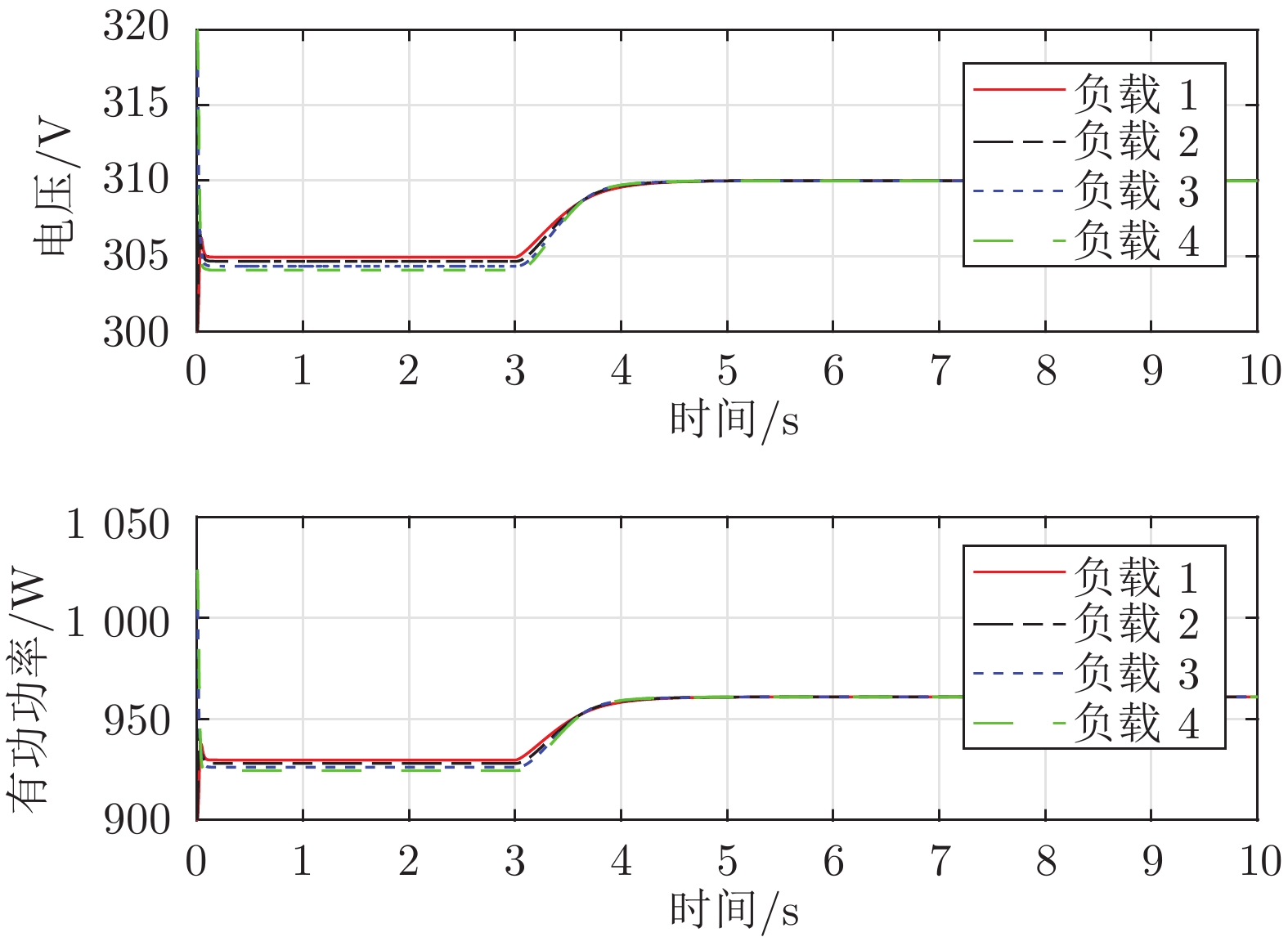
图 4 电压输出和恒定阻抗(Z)负载有功功率辨识结果
Fig. 4 Voltage output and identified real power of constant impedance load

图 5 电压输出和恒定电流(I)负载有功功率辨识结果
Fig. 5 Voltage output and identified real power of constant current load
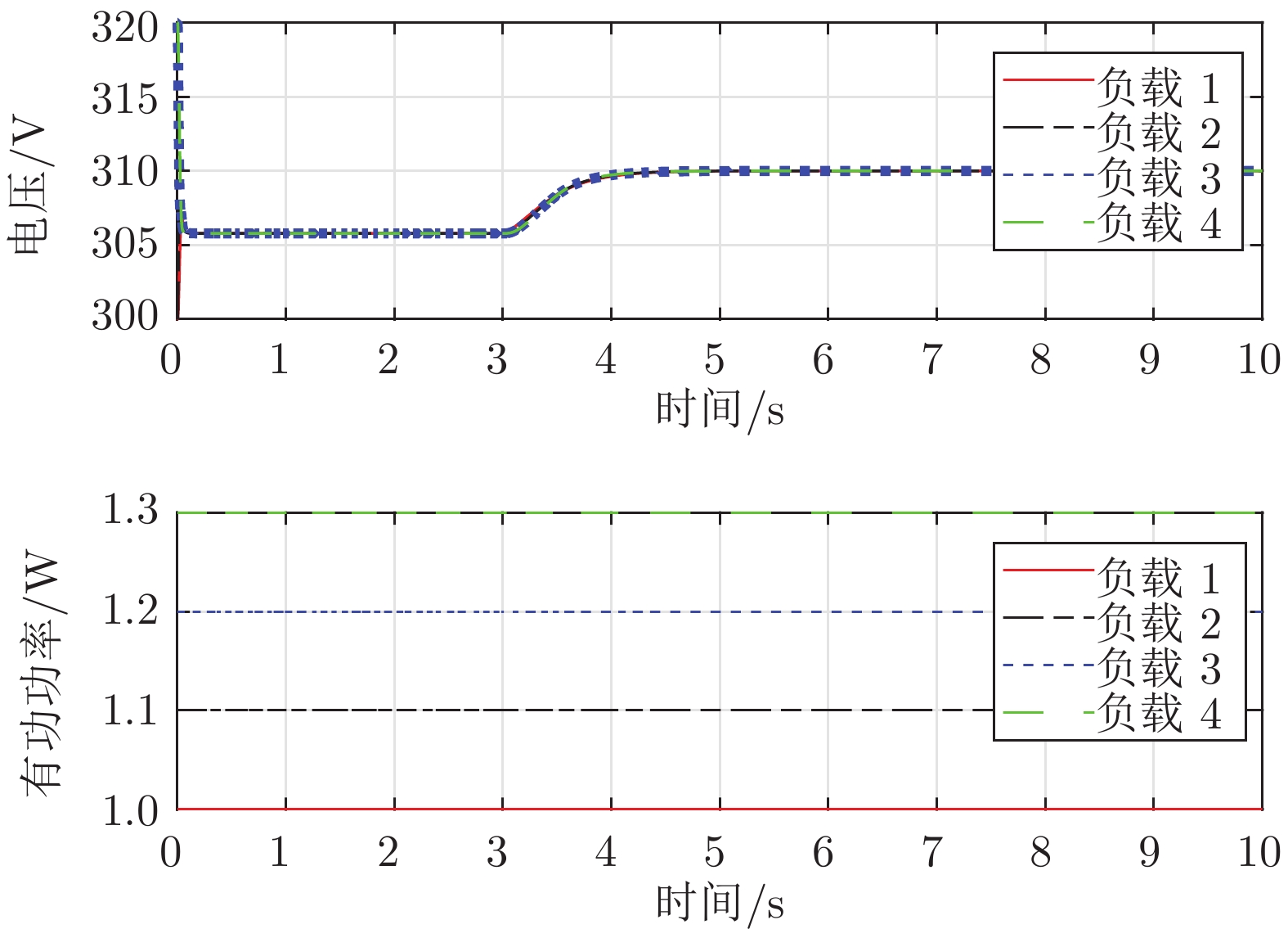
图 6 电压输出和恒定功率(P)负载有功功率辨识结果
Fig. 6 Voltage output and identified real power of constant power load
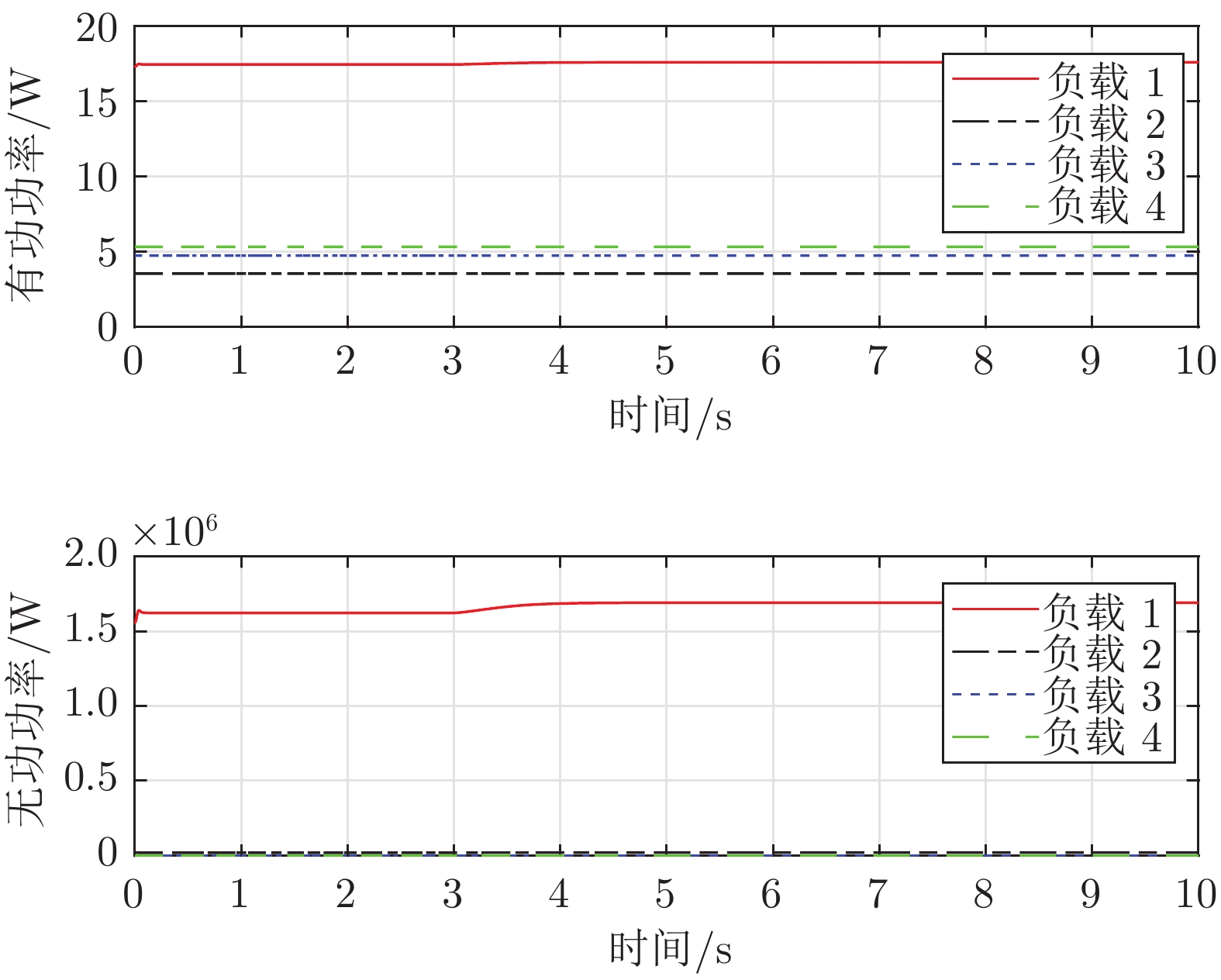
图 9 指数负载有功功率和无功功率辨识结果
Fig. 9 Identified real and reactive power output of exponential load
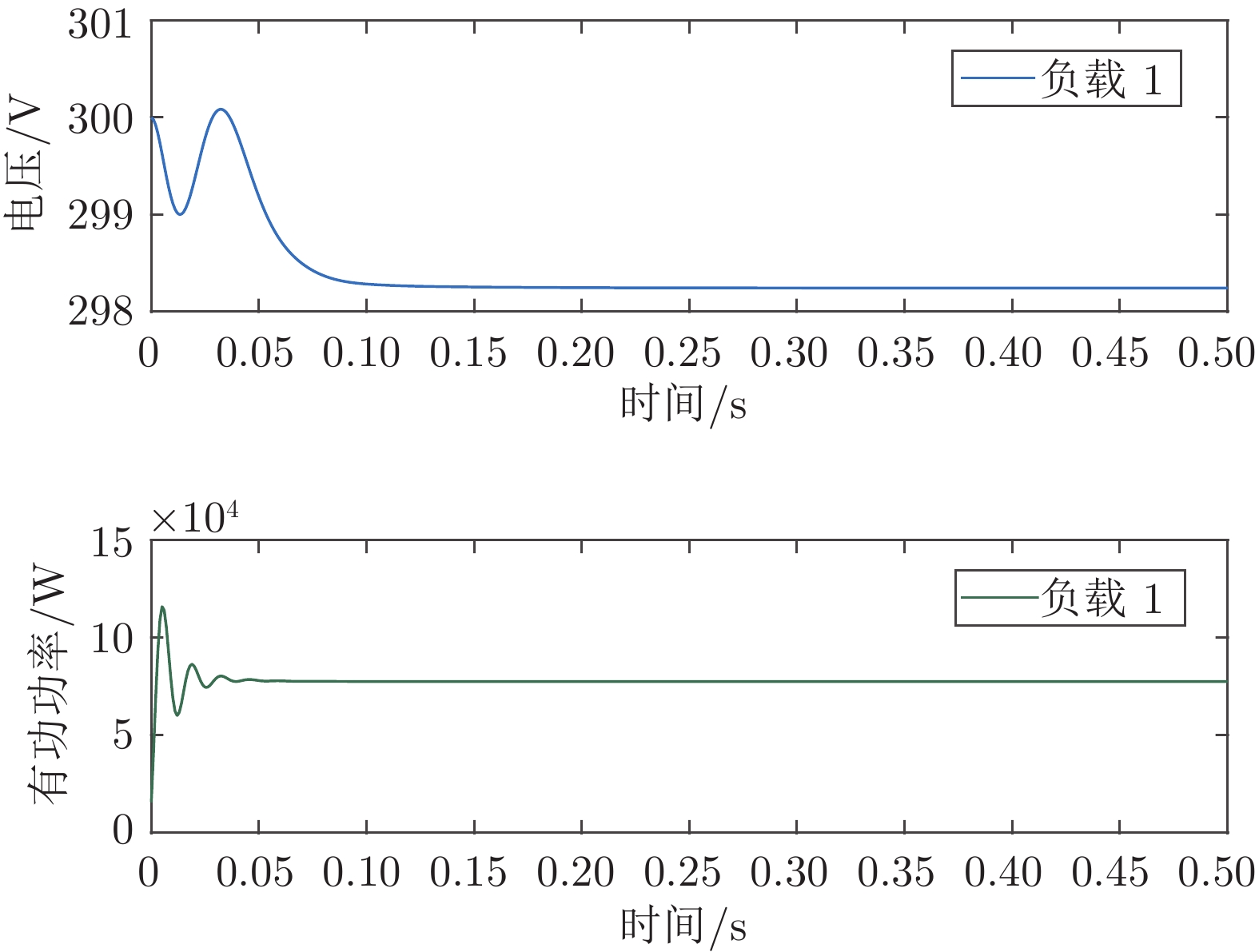
图 10 电压输出和动态负载有功功率辨识结果
Fig. 10 Voltage output and identified real power of dynamic load
表 1 不同负载元件指数值
$ n_p $ 和$ n_q $ [34]Table 1 Values of the exponents
$ n_p $ and$ n_q $ for different load components[34]负载元件/指数值 $ {n_p} $ $ {n_q} $ 空调 $ 0.50 $ $ 2.50 $ 电阻加热器 $ 2.00 $ $ 0.00 $ 灯 $ 1.00 $ $ 3.00 $ 泵机 $ 0.08 $ $ 1.60 $ 大型工业电机 $ 0.05 $ $ 0.50 $ 小型工业电机 $ 0.10 $ $ 0.60 $  下载: 导出CSV
表 2 输电线路参数
Table 2 Parameters of transmission lines
输电线路 线路1 线路2 线路3 $ \Omega^{-1} $ 10 10.67 9.82
下载: 导出CSV
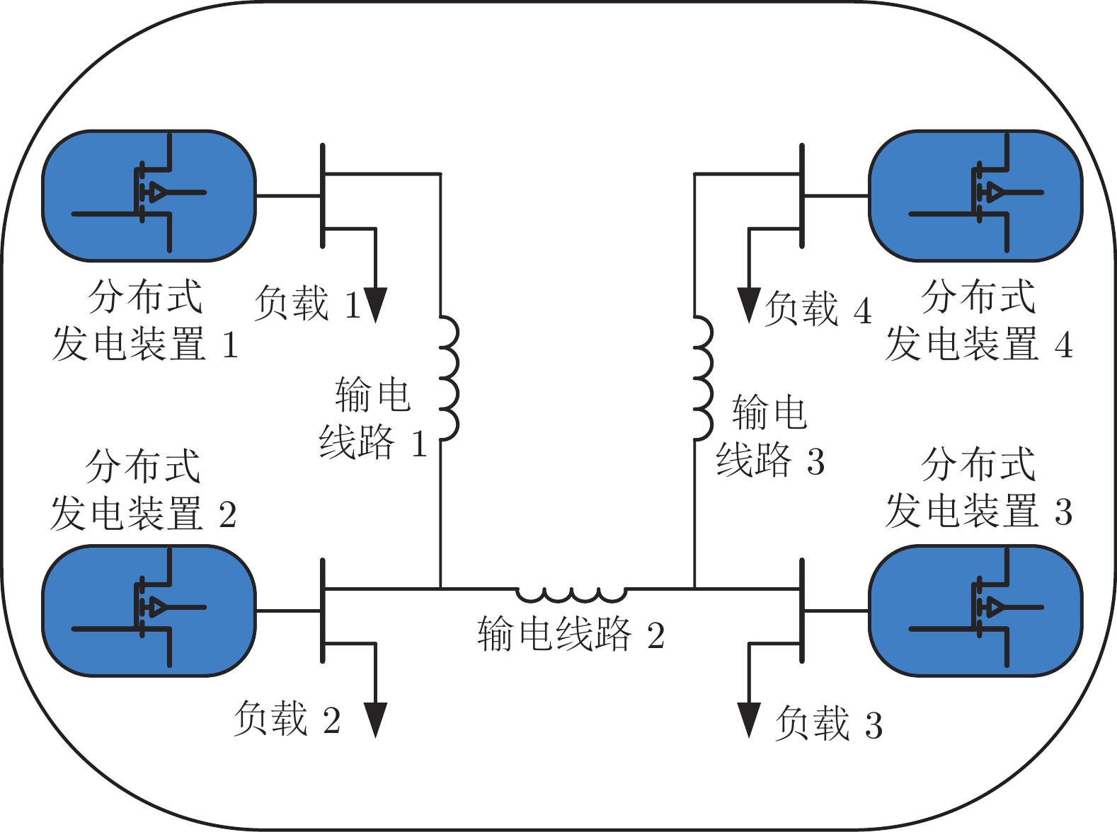
表 3 微电网系统参数
Table 3 Parameters of the islanded microgrid
参数 $ \mu G_1 $ $ \mu G_2 $ $ \mu G_3 $ $ \mu G_4 $ DG $ \tau_{P}(s) $ 0.16 0.16 0.16 0.16 $ K_{P}(s) $ $ 4\times 10^{-5} $ $ 2\times 10^{-5} $ $ 3\times 10^{-5} $ $ 4\times 10^{-5} $ $ \tau_{Q}(s) $ 0.16 0.16 0.16 0.16 $ K_{Q}(s) $ $ 4.2\times 10^{-4} $ $ 4.2\times 10^{-4} $ $ 4.2\times 10^{-4} $ $ 4.2\times 10^{-4} $ Load $ P_{Z} $ 0.01 0.02 0.03 0.04 $ P_{I} $ 1 2 3 4 $ P_{P} $ $ 1\times 10^{4} $ $ 1.1\times 10^{4} $ $ 1.2\times 10^{4} $ $ 1.3\times 10^{4} $ $ Q_{Z} $ 0.01 0.02 0.03 0.04 $ Q_{I} $ 1 2 3 4 $ Q_{P} $ $ 1\times 10^{4} $ $ 1.1\times 10^{4} $ $ 1.2\times 10^{4} $ $ 1.3\times 10^{4} $
下载: 导出CSV
表 4 负载Z, I, P稀疏辨识结果
Table 4 Sparse identification results for Z, I, P load
字典函数 Z I P 1 0 0 $1\times 10^{-4} $ $ V_1 $ 0 1.001 0 $ V_1^2 $ 0.098 0 0 $ V_1^3 $ 0 0 0 $ V_1^4 $ 0 0 0 1 0 0 $1.1\times 10^{-4} $ $ V_2 $ 0 1.998 0 $ V_2^2 $ 0.019 0 0 $ V_2^3 $ 0 0 0 $ V_2^4 $ 0 0 0 1 0 0 $1.2\times 10^{-4} $ $ V_3 $ 0 2.999 0 $ V_3^2 $ 0.031 0 0 $ V_3^3 $ 0 0 0 $ V_3^4 $ 0 0 0 1 0 0 $1.4\times 10^{-4} $ $ V_4 $ 0 3.999 0 $ V_4^2 $ 0.039 0 0 $ V_4^3 $ 0 0 0 $ V_4^4 $ 0 0 0
下载: 导出CSV
表 5 ZIP负载稀疏辨识结果
Table 5 Sparse identification results for ZIP load
字典函数 $ 1 $ $ V $ $ V^2 $ $ V^3 $ $ V^{3.5} $ $ V^4 $ $ V^6 $ 负载1 $1\times 10^{4}$ 1.001 0.011 0 0 0 0 负载2 $1.1\times 10^{4}$ 2.005 0.019 0 0 0 0 负载3 $1.2\times 10^{4}$ 2.993 0.029 0 0 0 0 负载4 $1.3\times 10^{4}$ 4.009 0.041 0 0 0 0
下载: 导出CSV
表 6 指数负载稀疏辨识结果
Table 6 Sparse identification results for exponential load
字典函数 $ 1 $ $ V^{0.05} $ $ V^{0.08} $ $ V^{0.1} $ $ V^{0.5} $ $ V $ $ V^{2.5} $ 空调 0 0 0 0 1 0 0 泵机 0 0 1 0 0 0 0 大型工业电机 0 1 0 0 0 0 0 小型工业电机 0 0 0 1 0 0 0
下载: 导出CSV
表 7 动态负载稀疏辨识结果
Table 7 Sparse identification results for dynamic load
字典函数 有功功率 无功功率 $ y(t) $ 1.0001 1.0001 $ q^{-1}y(t) $ −1.6003 −0.8997 $ q^{-2}y(t) $ 0.7998 0.5003 $ q^{-3}y(t) $ 0 0 $ q^{-4}y(t) $ 0 0 $ 1 $ 0.9002 0.8905 $ V(t) $ 0.4003 0.0984 $ V^2(t) $ 0.1727 0.4447 $ V^3(t) $ 0 0 $ V^4(t) $ 0 0
下载: 导出CSV
-
[1] 孙秋野, 滕菲, 张化光. 能源互联网及其关键控制问题. 自动化学报, 2017, 43(2): 176−194Sun Qiu-Ye, Teng Fei, Zhang Hua-Guang. Energy Internet and Its Key Control Issues. Acta Automatica Sinica, 2017, 43(2): 176−194 [2] R. H. Lasseter. Smart distribution: Coupled microgrids. Proceedings of the IEEE, 2011, 99(6): 1074−1082 doi: 10.1109/JPROC.2011.2114630 [3] Pepermans G, Driesen J, Haeseldonckx D, Belmans R, Dhaeseleer W. Distributed generation: Definition, benefits and issues. Energy Policy, 2005, 33(6): 787−798 doi: 10.1016/j.enpol.2003.10.004 [4] Sun Q Y, Han R K, Zhang H G, Zhou J G, Guerrero J M. A multiagent-based consensus algorithm for distributed coordinated control of distributed generators in the energy internet. IEEE Transactions on Smart Grid, 2015, 6(6): 3006−3019 doi: 10.1109/TSG.2015.2412779 [5] Sun Q Y, Zhang Y B, He H B, Ma D Z, Zhang H W. A novel energy function-based stability evaluation and nonlinear control approach for energy internet. IEEE Transactions on Smart Grid, 2017, 8(3): 1195−1210 doi: 10.1109/TSG.2015.2497691 [6] Zhang Y, Xie L, Ding Q F. Interactive control of coupled microgrids for guaranteed system-wide small signal stability. IEEE Transactions on Smart Grid, 2016, 7(2): 1088−1096 doi: 10.1109/TSG.2015.2495233 [7] Guedes R B L, Silva F H J R, Alberto L F C, Bretas N G. Large disturbance voltage stability assessment using extended Lyapunov function and considering voltage dependent active loads. In: Proceedings of the 2005 IEEE Power Engineering Society General Meeting. San Francisco, CA, USA: IEEE, 2005. 1760−1767 [8] Zhang K Q, Zhu H, Guo S M. Dependency analysis and improved parameter estimation for dynamic composite load modeling. IEEE Transactions on Power Systems, 2017, 32(4): 3287−3297 doi: 10.1109/TPWRS.2016.2623629 [9] Ballanti A, Ochoa L F. Voltage-led load management in whole distribution networks. IEEE Transactions on Power Systems, 2018, 33(2): 1544−1554 doi: 10.1109/TPWRS.2017.2716945 [10] Xu W, Vaahedi E, Mansour Y, Tamby J. Voltage stability load parameter determination from field tests on BC hydro's system. IEEE Transactions on Power Systems, 1997, 12(3): 1290−1297 doi: 10.1109/59.630473 [11] Knyazkin V, Cañizares C, Soder L. On the parameter estimation and modeling of aggregate power system loads. IEEE Transactions on Power Systems, 2004, 19(2): 1023−1031 doi: 10.1109/TPWRS.2003.821634 [12] Jazayeri P, Rosehart W, Westwick D T. Multistage algorithm for identification of nonlinear aggregate power system loads. IEEE Transactions on Power Systems, 2007, 22(3): 1072−1079 doi: 10.1109/TPWRS.2007.901281 [13] Ding F, Liu X P, Liu G J. Identification methods for Hammerstein nonlinear systems. Digital Signal Processing, 2011, 21(2): 215−238 doi: 10.1016/j.dsp.2010.06.006 [14] Karlsson D, Hill D J. Modelling and identification of nonlinear dynamic loads in power systems. IEEE Transactions on Power Systems, 1994, 9(1): 157−166 doi: 10.1109/59.317546 [15] Choi B K, Chiang H D, Li Y H, Li H, Chen Y T, Huang D H, Lauby M G. Measurement-based dynamic load models: Derivation, comparison, and validation. IEEE Transactions on Power Systems, 2006, 21(3): 1276−1283 doi: 10.1109/TPWRS.2006.876700 [16] Ju P, Handschin E, Karlsson D. Nonlinear dynamic loadmodelling: Model and parameter estimation. IEEE Transactions on Power Systems, 1996, 11(4): 1689−1697 doi: 10.1109/59.544629 [17] Rouhani A, Abur A. Real-time dynamic parameter estimation for an exponential dynamic load model. IEEE Transactions on Smart Grid, 2016, 7(3): 1530−1536 doi: 10.1109/TSG.2015.2449904 [18] Regulski P, Vilchis-Rodriguez D S, Djurovic S, Terzija V. Estimation of composite load model parameters using an improved particle swarm optimization method. IEEE Transactions on Power Delivery, 2015, 30(2): 553−560 doi: 10.1109/TPWRD.2014.2301219 [19] Miranian A, Rouzbehi K. Nonlinear power system load identification using local model networks. IEEE Transactions on Power Systems, 2013, 28(3): 2872−2881 doi: 10.1109/TPWRS.2012.2234142 [20] Bostanci M, Koplowitz J, Taylor C W. Identification of power system load dynamics using artificial neural networks. IEEE Transactions on Power Systems, 1997, 12(4): 1468−1473 doi: 10.1109/59.627843 [21] Chang G W, Chen C I, Liu Y J. A neural-network-based method of modeling electric arc furnace load for power engineering study. IEEE Transactions on Power Systems, 2010, 25(1): 138−146 doi: 10.1109/TPWRS.2009.2036711 [22] Lu C H. Wavelet fuzzy neural networks for identification and predictive control of dynamic systems. IEEE Transactions on Industrial Electronics, 2011, 58(7): 3046−3058 doi: 10.1109/TIE.2010.2076415 [23] Kontis E O, Papadopoulos T A, Chrysochos A I, Papagiannis G K. Measurement-based dynamic load modeling using the vector fitting technique. IEEE Transactions on Power Systems, 2018, 33(1): 338−351 doi: 10.1109/TPWRS.2017.2697004 [24] Arif A, Wang Z Y, Wang J H, Mather B, Bashualdo H, Zhao D B. Load modeling—A review. IEEE Transactions on Smart Grid, 2018, 9(6): 5986−5999 doi: 10.1109/TSG.2017.2700436 [25] Majumder R, Chaudhuri B, Ghosh A, Ledwich G, Zare F. Improvement of stability and load sharing in an autonomous microgrid using supplementary droop control loop. IEEE Transactions on Power Systems, 2010, 25(2): 796−808 doi: 10.1109/TPWRS.2009.2032049 [26] 孙秋野, 滕菲, 张化光, 马大中. 能源互联网动态协调优化控制体系构建. 中国电机工程学报, 2015, 35(14): 3667−3677Sun Qiu-Ye, Teng Fei, Zhang Hua-Guang, Ma Da-Zhong. Construction of dynamic coordinated optimization control system for energy internet. Proceedings of the CSEE, 2015, 35(14): 3667−3677 [27] 孙秋野, 王睿, 马大中, 刘振伟. 能源互联网中自能源的孤岛控制研究. 中国电机工程学报, 2017, 37(11): 3087−3098Sun Qiu-Ye, Wang Rui, Ma Da-Zhong, Liu Zhen-Wei. An islanding control strategy research of we-energy in energy internet. Proceedings of the CSEE, 2017, 37(11): 3087−3098 [28] Zhang Y, Xie L. A transient stability assessment framework in power electronic-interfaced distribution systems. IEEE Transactions on Power Systems, 2016, 31(6): 5106−5114 doi: 10.1109/TPWRS.2016.2531745 [29] Kolluri R R, Mareels I, Alpcan T, Brazil M, Hoog J, Thomas D A. Power sharing in angle droop controlled microgrids. IEEE Transactions on Power Systems, 2017, 32(6): 4743−4751 doi: 10.1109/TPWRS.2017.2672569 [30] Kundur P, Power System Stability and Control. New York: McGraw-Hill, 1994. [31] Bokhari A, Alkan A, Doğan R, Diaz-Aguilo M, De Leon F, Czarkowski D, Zabar Z, Birenbaum L. Experimental determination of the ZIP coefficients for modern residential, commercial, and industrial loads. IEEE Transactions on Power Delivery, 2013, 29(3): 1372−1381 [32] Collin A J, Tsagarakis G, Kiprakis A E, McLaughlin S. Development of low-voltage load models for the residential load sector. IEEE Transactions on Power Systems, 2014, 29(5): 2180−2188 doi: 10.1109/TPWRS.2014.2301949 [33] Milanovic J V, Yamashita K, Villanueva S M, Djokic S Z, Korunovic L M. International industry practice on power system load modeling. IEEE Transactions on Power Systems, 2013, 28(3): 3038−3046 doi: 10.1109/TPWRS.2012.2231969 [34] Hatipoglu K, Fidan I, Radman G. Investigating effect of voltage changes on static ZIP load model in a microgrid environment. In: Proceedings of the Conference on North American Power Symposium. Champaign, USA: IEEE, 2012. 1−5 [35] Bao Y, Wang L Y, Wang C S, Wang Y. Hammerstein models and real-time system identification of load dynamics for voltage management. IEEE Access, 2018, 6: 34598−34607 doi: 10.1109/ACCESS.2018.2849002 [36] Pan W, Yuan Y, Goncalves J, Stan G B. A sparse Bayesian approach to the identification of nonlinear state-space systems. IEEE Transactions on Automatic Control, 2016, 61(1): 182−187 doi: 10.1109/TAC.2015.2426291 [37] Qu Q, Sun J, Wright J. Finding a sparse vector in a subspace: linear sparsity using alternating directions. IEEE Transactions on Information Theory, 2016, 62(10): 5855−5880 doi: 10.1109/TIT.2016.2601599 [38] Palmer J A, Kreutz-Delgado K, Wipf D P, Rao B D. Variational EM algorithms for non-Gaussian latent variable models. Advances in Neural Information Processing Systems, 2006, 18: 1059−1066 [39] Zhang Z, Xu Y, Yang J, Li X L, Zhang D. A survey of sparse representation: Algorithms and applications. IEEE Access, 2015, 3(1): 490−530 [40] Guo F H, Wen C Y, Mao J F, Song Y D. Distributed secondary voltage and frequency restoration control of droop-controlled inverter-based microgrids. IEEE Transactions on Industrial Electronics, 2015, 62(7): 4355−4364 doi: 10.1109/TIE.2014.2379211 -

 下载:
下载:


计量
- 文章访问数: 2031
- HTML全文浏览量: 1431
- PDF下载量: 332
- 被引次数: 0
