

Two-order Approximate Spectral Convolutional Model for Semi-Supervised Classification
-
摘要:
近年来, 基于局部一阶近似的谱图卷积方法在半监督节点分类任务上取得了明显优势, 但是在每次更新节点特征表示时, 只利用了一阶邻居节点信息而忽视了非直接邻居节点信息. 为此, 本文结合切比雪夫截断展开式及标准化的拉普拉斯矩阵, 通过推导及简化二阶近似谱图卷积模块, 提出了一种融合丰富局部结构信息的改进图卷积模型, 进一步提高了节点分类性能. 大量的实验结果表明, 本文提出的方法在不同数据集上的表现均优于现有的流行方法, 验证了模型的有效性.
Abstract:In recent years, the spectral convolution method based on local first-order approximation has achieved significant advantages in semi-supervised node classification tasks. However, when updating the node feature representation at each stage, only the first-order neighbor node information is used, while the indirect neighbor node information is ignored. To this end, this paper combines Chebyshev′ s truncated expansion and symmetric normalized Laplacian matrix, and by deducing and simplifying the two-order approximate spectral convolution module, an improved graph convolution model is proposed which fuses rich local structure information. A large number of experimental results show that the method proposed in this paper is superior to the existing popular methods on different datasets, which verifies the effectiveness of the model.
-
Key words:
- Graph theory /
- spectral convolution /
- semi-supervised learning /
- node classification /
- relational data
-

图 1 本文构造的二阶邻域谱图卷积网络描述图
Fig. 1 A schematic diagram of our two-order neighborhood spectral convolution network
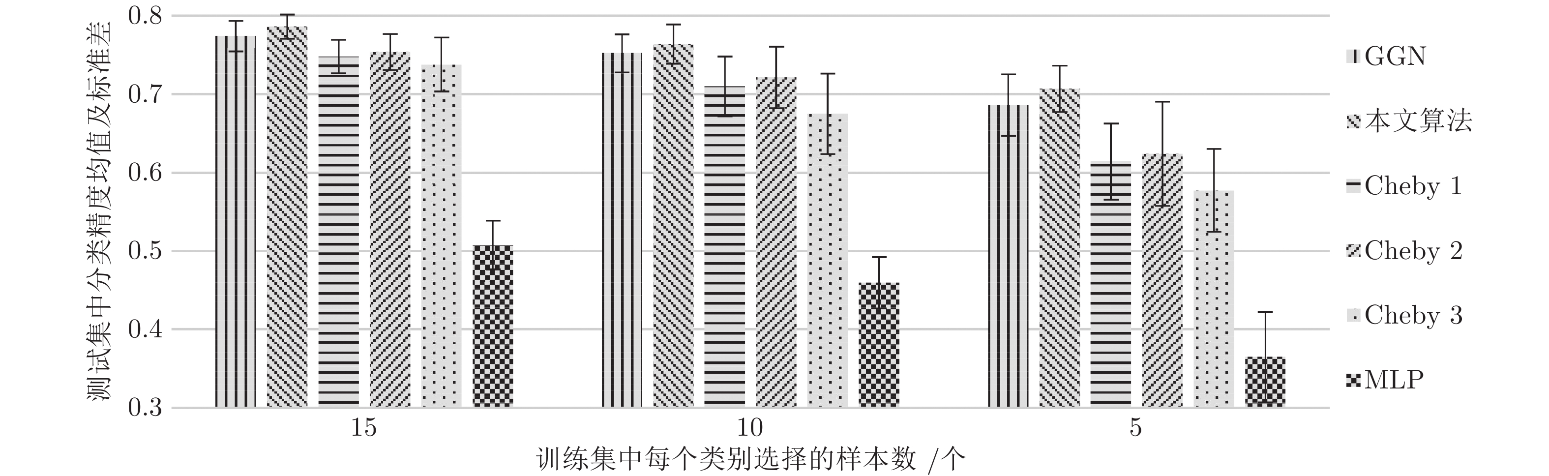
图 2 Cora上不同训练集大小(每个类的标记节点数)的准确率
Fig. 2 Accuracy for different training set sizes (number of labeled nodes per class) on Cora
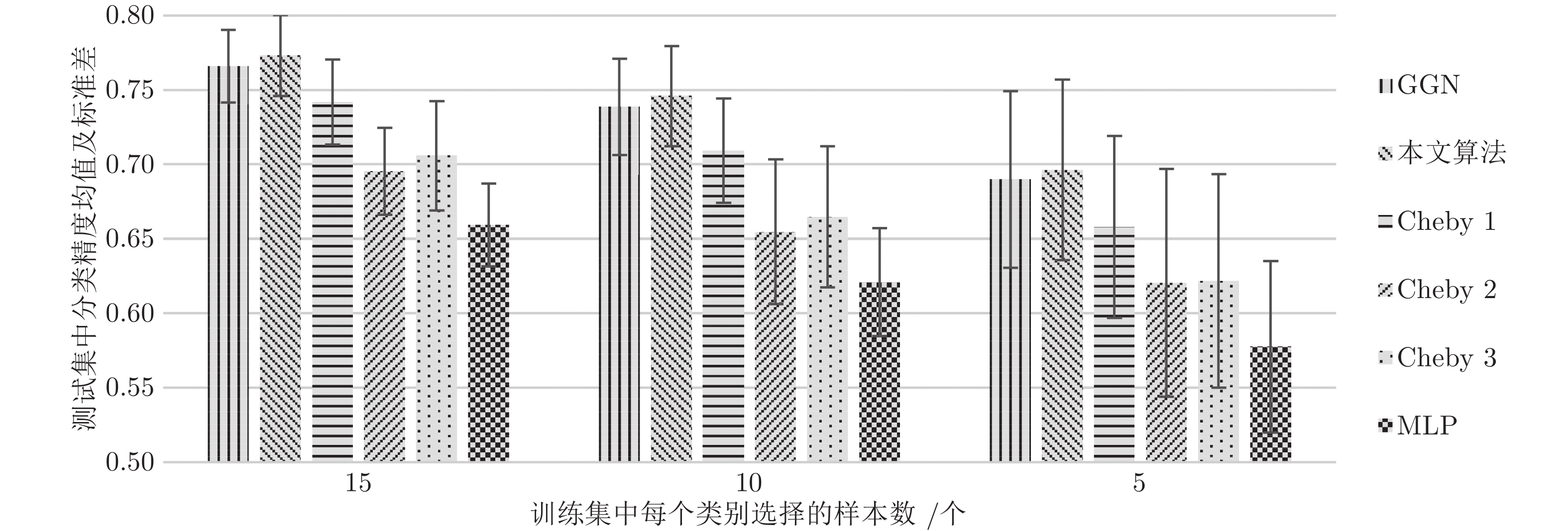
图 4 PubMed上不同训练集大小(每个类的标记节点数)的准确率
Fig. 4 Accuracy for different training set sizes (number of labeled nodes per class) on PubMed

图 3 CiteSeer上不同训练集大小(每个类的标记节点数)的准确率
Fig. 3 Accuracy for different training set sizes (number of labeled nodes per class) on CiteSeer

图 5 目标节点t的一阶及两阶邻域组成的局部网络示意图
Fig. 5 Schematic diagram of local network composed of the first-order and two-order neighborhoods of target node t
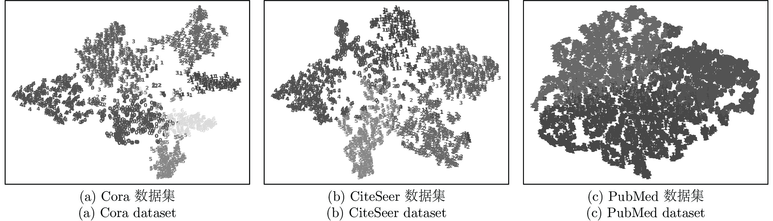
图 6 在3个数据集上模型隐含层学习到的隐特征表示的t-SNE图
Fig. 6 A t-SNE plot of the learned hidden feature representations of the model’s hidden layer on the three datasets
表 1 4个数据集的基本统计信息
Table 1 Basic statistics information for four datasets
数据集 节点 边 特征 类别 CiteSeer 3327 4732 3703 6 Cora 2708 5429 1433 7 PubMed 19717 44338 500 3 NELL 65755 266144 5414 210  下载: 导出CSV
表 2 分类准确率结果汇总(%)
Table 2 Summary of results in terms of classification accuracy (%)
算法 CiteSeer Cora PubMed NELL ManiReg 60.1 59.5 70.7 21.8 SemiEmb 59.6 59.0 71.1 26.7 LP 45.3 68.0 63.0 26.5 DeepWalk 43.2 67.2 65.3 58.1 ICA 69.1 75.1 73.9 23.1 Planetoid 64.7 75.7 77.2 61.9 SpectralCNN 58.9 73.3 73.9 — Cheby-Net 69.8 81.2 74.4 — Monet — 81.7 78.8 — GCN 70.3 81.5 79.0 66.0 本文算法 71.8 82.6 79.8 67.2
下载: 导出CSV
-
[1] Meng Z Q, Liang S S, Bao H Y, Zhang X L. Co-embedding attributed networks. In: Proceedings of the 12th ACM International Conference on Web Search and Data Mining, New York, NY, USA: ACM, 2019. 393−401 [2] Kipf T N, Welling M. Semi-supervised classification with graph convolutional networks. In: Proceedings of the 5th International Conference on Learning Representations, Toulon, France: OpenReview, 2017. 1−14 [3] Liu Z Q, Chen C C, Yang X X, Zhou J, Li X L, Song L. Heterogeneous graph neural networks for malicious account detection. In: Proceedings of the 27th International Conference on Information and Knowledge Management, New York, NY, USA: ACM, 2018. 2077−2085 [4] Zhu X J, Ghahramani Z, Lafferty J D. Semi-supervised learning using Gaussian fields and harmonic functions. In: Proceedings of the 20th International Conference on Machine Learning, Menlo Park, CA, USA: AAAI, 2003. 912−919 [5] Talukdar P P, Crammer K. New regularized algorithms for transductive learning. In: Proceedings of the 2009 European Conference on Machine Learning and Principles and Practice of Knowledge Discovery in Databases, Berlin, Germany: Springer, 2009. 442−457 [6] Belkin M, Niyogi P, Sindhwani V. Manifold regularization: A geometric framework for learning from labeled and unlabeled examples. Journal of Machine Learning Research, 2006, 7(11): 2399−2434 [7] Weston J, Frédéric R, Collobert R. Deep learning via semi-supervised embedding. In: Proceedings of the 25th International Conference on Machine Learning, Berlin, Germany: Springer, 2012. 639−655 [8] Lu Q, Getoor L. Link-based classification. In: Proceedings of the 20th International Conference on Machine Learning, Menlo Park, CA, USA: AAAI, 2003. 496−503 [9] Perozzi B, Al-Rfou R, Skiena S. Deepwalk: Online learning of social representations. In: Proceedings of the 20th ACM SIGKDD International Conference on Knowledge Discovery and Data Mining, New York, NY, USA: ACM, 2014. 701−710 [10] Tang J, Qu M, Wang M Z, Zhang M, Yan J, Mei Q Z. Line: Large-scale information network embedding. In: Proceedings of the 24th International Conference on World Wide Wed, New York, NY, USA: ACM, 2015. 1067−1077 [11] Grover A, Leskovec J. Node2vec: Scalable feature learning for networks. In: Proceedings of the 22nd ACM SIGKDD International Conference on Knowledge Discovery and Data Mining, New York, NY, USA: ACM, 2016. 855−864 [12] Yang Z L, Cohen W W, Salakhutdinov R. Revisiting semi-supervised learning with graph embeddings. In: Proceedings of the 33rd International Conference on Machine Learning, Cambridge, MA, USA: MIT Press, 2016. 40−48 [13] Mikolov T, Sutskever I, Chen K, Corrado G S, Dean J. Distributed representations of words and phrases and their compositionality. In: Proceedings of the 27th Annual Conference on Neural Information Processing Systems, New York, NY, USA: Curran Associates, 2013. 3111−3119 [14] Sun K, Xiao B, Liu D, Wang J D. Deep high-resolution representation learning for human pose estimation. In: Proceedings of the 2019 IEEE Conference on Computer Vision and Pattern Recognition, New York, USA: IEEE, 2019. 5693−5703 [15] Zhang Y, Pezeshki M, Brakel P, Zhang S Z, Laurent C, Bengio Y, et al. Towards end-to end speech recognition with deep convolutional neural networks. In: Proceedings of the 17th Annual Conference of the International Speech Communication Association, New York, USA: Elsevier 2016. 410−414 [16] Niepert M, Ahmed M, Kutzkov K. Learning convolutional neural networks for graphs. In: Proceedings of the 33rd International Conference on Machine Learning, Cambridge, MA, USA: MIT Press, 2016. 2014−2023 [17] Velickovic P, Cucurull G, Casanova A, Romero A, Liò P, Bengio Y. Graph attention networks. In: Proceedings of the 6th International Conference on Learning Representations, Vancouver, BC, Canada: OpenReview, 2018. 1−12 [18] Gao H Y, Wang Z Y, Ji S W. Large-scale learnable graph convolutional networks. In: Proceedings of the 24th ACM SIGKDD International Conference on Knowledge Discovery and Data Mining, New York, NY, USA: ACM, 2018. 1416−1424 [19] Hamilton W L, Ying Z T, Leskovec J. Inductive representation learning on large graphs. In: Proceedings of the 31st Annual Conference on Neural Information Processing Systems, New York, NY, USA: Curran Associates, 2017. 1024−1034 [20] Bruna J, Zaremba W, Szlam A, Lecun Y. Spectral networks and locally connected networks on graphs. In: Proceedngs of the 2nd International Conference on Learning Representations, Banff, AB, Canada: OpenReview, 2014. 1−14 [21] Defferrard M, Bresson X, Vandergheynst P. Convolutional neural networks on graphs with fast localized spectral filtering. In: Proceedings of the 29th Annual Conference on Neural Information Processing Systems, New York, NY, USA: Curran Associates, 2016. 3844−3852 [22] Hammond D K, Vandergheynst P, Rémi G. Wavelets on graphs via spectral graph theory. Applied and Computational Harmonic Analysis, 2012, 30(2): 129−150 [23] Li Q M, Han Z C, Wu X M. Deeper insights into graph convolutional networks for semi-supervised learning. In: Proceedings of the 32nd AAAI Conference on Artificial Intelligence, Menlo Park, CA, USA: AAAI, 2018. 3538−3545 [24] Shuman D I, Narang S K, Frossard P, Ortega A, Vandergheynst P. The emerging field of signal processing on graphs: Extending high-dimensional data analysis to networks and other irregular domains. IEEE Signal Processing Magazine, 2013, 30(3): 83−98 doi: 10.1109/MSP.2012.2235192 [25] Giles C L, Bollacker K, Lawrence S. Citeseer: An automatic citation indexing system. In: Proceedings of the 3rd ACM International Conference on Digital Libraries, New York, NY, USA: ACM, 1998. 89−98 [26] McCallum A, Nigam K, Rennie J, Seymore K. Automating the construction of internet portals with machine learning. Information Retrieval, 2000, 3(2): 127−163 doi: 10.1023/A:1009953814988 [27] Namata G, London B, Getoor L, Huang B. Query-driven active surveying for collective classification. In: Proceedings of the 10th workshop on Mining and Learning with Graphs, Edinburgh, Scotland: ACM, 2012. 1−8 [28] Andrew C, Justin B, Bryan K, Burr S, Estevam R H J, Tom M M. Toward an architecture for never-ending language learning. In: Proceedings of the 24th AAAI Conference on Artificial Intelligence, Menlo Park, CA, USA: AAAI, 2010. 1306−1313 [29] Glorot X, Bengio Y. Understanding the difficulty of training deep feedforward neural networks. In: Proceedings of the 13th International Conference on Artificial Intelligence and Statistics, Cambridge, MA, USA: MIT Press, 2010. 249−256 [30] Kingma D P, Ba J. Adam: A method for stochastic optimization. In: Proceedings of the 3rd International Conference on Learning Representations, San Diego, CA, USA: OpenReview, 2015. 1−15 [31] Srivastava N, Hinton G, Krizhevsky A, Sutskever I, Salakhutdinov R. Dropout: A simple way to prevent neural networks from overfitting. Journal of Machine Learning Research, 2014, 15(1): 1929−1958 [32] Monti F, Boscaini D, Masci J, Rodola E, Svoboda J, Bronstein M M. Geometric deep learning on graphs and manifolds using mixture model CNNs. In: Proceedings of the 2017 IEEE Conference on Computer Vision and Pattern Recognition, New York, USA: IEEE, 2017. 5425−5434 [33] Van der Maaten L, Hinton G. Visualizing data using t-SNE. Journal of Machine Learning Research, 2008, 9(11): 2579−2605 -

 下载:
下载:

计量
- 文章访问数: 945
- HTML全文浏览量: 421
- PDF下载量: 193
- 被引次数: 0
