

Two-order Approximate Spectral Convolutional Model for Semi-Supervised Classification
-
摘要:
近年来, 基于局部一阶近似的谱图卷积方法在半监督节点分类任务上取得了明显优势, 但是在每次更新节点特征表示时, 只利用了一阶邻居节点信息而忽视了非直接邻居节点信息. 为此, 本文结合切比雪夫截断展开式及标准化的拉普拉斯矩阵, 通过推导及简化二阶近似谱图卷积模块, 提出了一种融合丰富局部结构信息的改进图卷积模型, 进一步提高了节点分类性能. 大量的实验结果表明, 本文提出的方法在不同数据集上的表现均优于现有的流行方法, 验证了模型的有效性.
Abstract:In recent years, the spectral convolution method based on local first-order approximation has achieved significant advantages in semi-supervised node classification tasks. However, when updating the node feature representation at each stage, only the first-order neighbor node information is used, while the indirect neighbor node information is ignored. To this end, this paper combines Chebyshev′ s truncated expansion and symmetric normalized Laplacian matrix, and by deducing and simplifying the two-order approximate spectral convolution module, an improved graph convolution model is proposed which fuses rich local structure information. A large number of experimental results show that the method proposed in this paper is superior to the existing popular methods on different datasets, which verifies the effectiveness of the model.
-
Key words:
- Graph theory /
- spectral convolution /
- semi-supervised learning /
- node classification /
- relational data
-
随着信息科技的快速发展与推广, 人们收集、存储数据的能力得到了飞速提升. 在很多实际任务中我们可以很容易地获取大量未标记(Unlabeled)的数据, 而标记数据往往是极其昂贵和耗时的, 因此“标记数据少, 未标记数据多”的现象较为明显. 若只使用少量有标记样本进行学习, 而忽略大量未标记数据是对数据资源的浪费. 此外, 由于图结构能够很自然地用于对社交关系、生物分子结构及出版物引用关系等复杂系统建模, 因此以半监督学习的方式分析基于图建模的这类问题是非常关键且有意义的. 节点分类作为图分析中的一项重要研究, 受到了越来越多研究者的关注, 并广泛用于社交关系网络的用户画像[1]、引文网络的文献分类[2]、风控系统中的异常检测[3]等领域.
近年来, 国内外学者提出了很多基于图的传统的学习方法用来有效地解决节点分类问题, 这类方法通常将问题用一个包括节点及边的图
$ G\left( {V,E} \right) $ 来建模, 图上的节点集$ V $ 表示样本, 每个节点一般会有一些特征描述且与某个固定的类别标签相关联, 而边集$ E $ 一般是有权值的, 并且权值的大小表示样本之间的相似性程度. 当给定部分有标记的图时, 通过使用少量有标记的数据和大量无标记数据的特征信息在已构建的图结构上共同学习一个模型, 从而实现对未标记节点的分类. 基于图的传统分类方法, 在发展过程中主要形成了以下分支, 一类是基于标签传播思想的设计方法[4-8]; 另一类是基于图嵌入的方法[9-12]. 基于标签传播思想的方法主要是将有标记样本的标签信息在图上传播, 并利用图拉普拉斯正则项约束有较大边权重的相邻节点具有相同的类别. Zhu等[4]提出的标签传播(Label propagation)方法, 使用一个约束的标签分配函数, 对每个未标记样本实例选择相邻节点中类别标签数量最多的作为自己的标签类型, 随着类别标签的不断传播, 使得最终紧密相连的节点数据有相同的类别标签. Talukdar等[5]提出的方法是标签传播方法的一种变体, 它允许对已标记节点的预测标签进行改变, 引入了节点的不确定性, 这种设计方式解决了标签传播算法中某些已标记信息是噪声却无法在传播过程中对其进行修复的问题. Belkin等[6]提出了流行正则(Manifold regularization)方法, 目标函数设计时考虑了再生核希尔伯特空间(Reproducing kernel Hilbert spaces, RKHS)中参数化的核函数且正则项中引入了样本的几何边缘分布信息. Weston等[7]提出的半监督嵌入(Semi-supervised embedding)方法将适用于浅层半监督学习技术(如内核方法)的非线性嵌入算法应用到了深层结构中, 并且拓展了目标函数的正则项. 迭代分类算法(Iterative classification algorithm, ICA)[8]则是在评估局部分类器与分配新标签之间采用一个迭代的过程, 在每次迭代时, 根据其相邻节点的当前预测标签对图上节点数据进行分类.基于图嵌入的方法, 其主要动机是希望对每个节点学习一个低维的向量表示, 同时使该向量表示尽可能的保持原来的拓扑结构关系及特征属性. Perozzi等[9]提出的深度游动(Deepwalk)算法作为经典的图嵌入方法, 它在图上利用随机游动的路径构造节点序列, 然后使用SkipGram模型[13]更新学习节点的表示, 最终利用学习到的低维向量实现对图上节点数据的分类. Line[10]和Node2Vec[11]方法则使用更复杂的随机游动模型或广度优先搜索策略进一步拓展了深度游动算法. Yang等[12]提出了基于图嵌入的半监督学习框架, 通过注入类别标签的方式来学习每个节点的嵌入表示, 实现对图上节点的分类.
虽然基于图的传统的分类方法在节点分类任务上已取得了一定的分类效果, 但是这类方法仍存在着一些不足. 例如标签传播等算法在对未标记节点分类时只使用了类别标签和图结构信息, 而没有利用节点本身的特征属性信息. 深度游动等算法只使用了图结构信息来学习低维特征表达, 没有利用标签信息来辅助节点表示的学习. 没有充分利用已有的信息会使最终分类精度及泛化性能受到较大影响.
近几年来, 卷积神经网络在计算机视觉[14]、语音识别[15]等机器学习任务上取得了巨大的成功, 但由于图数据的每个节点邻域大小不一, 基于核的卷积在网格上的平稳性已无法满足, 因此无法直接将卷积神经网络用到图分析问题上, 如何将卷积网络拓展到处理图数据的研究得到了越来越多的关注. 根据卷积定义方式的不同, 将卷积神经网络推广到图数据的方法概括为以下类别: 一类是空间域上的卷积方法[16-19]; 另一类是谱域上的卷积方法[2, 20-21]. 空间域上的卷积方法是在图的节点上直接定义卷积, 该方法遵循了传统卷积神经网络的做法. 对于图上的每个节点, 卷积被定义为对其邻域内所有节点的加权平均函数, 且加权函数表征了邻域对目标节点的影响. 该类方法的主要困难在于如何定义一个卷积算子来处理不同邻域大小的节点数据, 并且保持卷积神经网络权值共享的属性. Niepert等[16]提出了一种从任意图结构中提取局部连通区域的通用方法, 不过其采用的方法是将局部图先转换为一维的序列然后再使用传统的一维卷积进行处理, 该方法的主要缺点是转换序列之前需要首先定义节点的优先顺序. Velickovic等[17]提出图关注网络(Graph attention network)方法, 采用注意力机制学习中心节点与每个相邻节点特征向量之间的相关性来获得不同的权重, 并通过特征权重来聚合相邻节点的特征表示. Gao等[18]提出的大规模可学习图网络(Large-scale learnable GCN)方法, 通过对邻域节点的单个特征值大小排序以实现数据预处理, 训练时采用传统的卷积方法. 图采样与聚合(Graph sample and aggregate)方法[19]从一阶邻居中采样固定数量的邻居节点, 并使用某种聚集方法(如平均值、最大池化或LSTM等)将采样节点信息聚合来更新中心节点的特征表示, 其在大规模图上表现出了较好的性能.
而谱域上的卷积方法基于图傅里叶变换[22]及卷积理论等, 先将图上的节点数据及滤波器变换到谱域中进行运算, 然后再将谱域上得到的乘积结果通过图傅里叶逆变换转回到空间域得到最终卷积结果. 该类方法首先由Bruna等[20]提出, 之后Defferrard等[21]使用多项式近似谱滤波器的方式加速了卷积运算. Kipf等[2]使用一阶线性逼近, 进一步简化了计算, 取得了较好的分类效果. 但是通常该类方法节点的邻域组成较为简单, 每次聚集节点特征时只考虑到直接相连的邻居节点信息, 而忽视了非直接相连的邻域信息, 因此每次提取节点特征时不能够充分利用到丰富的图结构信息, 导致忽略了某些潜在的有利信息. 即使可通过堆叠多层网络实现对二阶及更高阶邻居节点信息的整合, 但是由于图卷积网络采用多层消息聚合的方案, 当堆叠多层网络后往往导致过平滑现象而使分类性能不增反降[23]. 目前GCN通常局限于浅层网络, 一般使用2层网络时分类效果最好, 虽然为了加深网络可以使用残差连接等技巧, 但即使使用了这些技巧, 也只是勉强保持性能不下降, 并没有提高性能.
针对这些问题, 本文希望在保持浅层网络的前提下, 能更好地利用到更丰富的结构信息来实现对节点特征表示的学习, 提升最终的节点分类效果. 本文提出在利用切比雪夫二阶截断展开多项式构造卷积模块的基础上, 精简模型参数, 并进行重标准化等优化处理, 使得构造的二阶近似谱图卷积模块在每次更新节点特征表示时能够更有效地融合二阶邻居节点的特征信息, 从而进一步提高节点分类的精度.
1. 二阶近似谱图卷积网络模型
本文提出了一种用于对图节点分类的二阶邻域近似谱图卷积网络模型, 总体框架描述图如图1所示. 该网络模型共包含两层(隐层和输出层), 网络的输入数据为节点的属性矩阵
${X_{{\rm{in}}}} \in {{\bf{R}}^{N \times C}},$ 它表示含有$ N $ 个节点且每个节点使用$ C $ 维向量进行描述的属性矩阵. 隐层(Hidden layer)使用本文设计的二阶近似谱图卷积模块提取节点的隐特征表示, 然后对得到的隐特征表示做非线性激活, 得到隐层输出Hout$\in {{\bf{R}}^{N \times H}} ,$ 其中H为隐层特征维数, 并把结果送入网络的输出层(Output layer), 在输出层中使用构造的卷积模块对从隐层送入的数据做卷积处理, 然后通过分类函数(Softmax function)预测每个节点的类别分布, 得到Oout$\in {{\bf{R}}^{N \times W}}, $ 其中W为类别个数, 最终实现对节点的分类. 图 1 本文构造的二阶邻域谱图卷积网络描述图Fig. 1 A schematic diagram of our two-order neighborhood spectral convolution network
下面分别从谱图卷积理论基础、二阶近似卷积模块设计、分层前向传播网络实现及模型的损失函数构造等几个方面对本文提出的模型进行详细阐述.
1.1 谱图卷积基础
令
$ G\left( {V,E} \right) $ 表示一个无向权重图, 其中$ V $ 是顶点集,$ E \subseteq V \times V $ 是边集,$ {{A}} \in {{\bf{R}}^{N \times N}} $ 表示图的邻接矩阵,$ {{{x}}} \in {{\bf{R}}^N} $ 表示图信号, 它的第$ i $ 个分量$ {{ x}_i} $ 表示$ V $ 中第$ i $ 个顶点的信号值. 标准化的图拉普拉斯矩阵被定义为$ L={I_N} - {D^{ - \frac{1}{2}}}A{D^{ - \frac{1}{2}}}, $ 其中$ {I_N} $ 是$ N $ 阶的单位矩阵,$ D \in {{\bf{R}}^{N \times N}} $ 是对角矩阵且对角元素值$ {D_{ii}}=\sum\nolimits_j {{A_{ij}}} $ .$ L $ 存在一组正交的特征向量$ \left\{ {{{ {{u}}}_{{i}}}} \right\}_{i=0}^{N - 1} \in $ ${{\bf{R}}^N} $ 和对应的非负特征值$ \left\{ {{\lambda _i}} \right\}_{i=0}^{N - 1} $ . 由于$ L $ 为对称矩阵可对角化, 经谱分解有$L=U\Lambda {U^{\rm{T}}},$ 其中$ \Lambda=$ ${\rm{diag}}\left\{ { {{\lambda _0},{\lambda _1}, \cdots ,{\lambda _{N - 1}}} } \right\}\! \in\! {{\bf{R}}^{N \times N}}.$ 当给定图上的一个信号
${{x}} \in {{\bf{R}}^N},$ $ {{x}} $ 经图傅里叶变换后, 得到$ {\hat{ x}}={U^{\rm{T}}}{{x}} \in {{\bf{R}}^N} $ [24]. 图傅里叶变换使我们能够应用图滤波器$ g $ 实现对图信号$ {{x}} $ 的谱图卷积. 具体表示为$$ {g} * {{{x}}}=Ug\left( \Lambda \right){U^{\rm{T}}}{{{x}}}=Ug\left( \Lambda \right){\hat{ x}} $$ (1) 其中,
$* $ 代表卷积运算,$g(\Lambda )\!=\!{\rm{diag}}\{ g( {{\lambda _0}} ),g( {{\lambda _1}} ), \cdots , $ $ g( {{\lambda _{N - 1}}}) \} ,$ 它控制图信号$ {{x}} $ 中每个分量的频率如何改变. 然而通过式(1)应用图滤波对信号$ {{x}} $ 进行处理, 需要对$ L $ 进行谱分解, 因此需要较高的计算代价.Hammond等[22]首先证明了使用切比雪夫多项式可以较好地近似
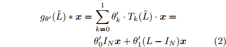
$ g(\lambda ) $ . 之后, Defferrard等[21]使用切比雪夫多项式拟合卷积核构建用于图分类的卷积神经网络. 而GCN方法[2]作为一阶近似谱图卷积方法, 利用切比雪夫一阶截断展开式构造了谱图卷积模型. 首先它利用递推式构造基础卷积模块为$$ \begin{split} {g_{\theta {'}}}({{\tilde L}}) * {{{x}}} =\,&\sum\limits_{k=0}^1 {{\theta '_k} \cdot {T_k}{\rm{(}}{{\tilde L}}{\rm{)}} \cdot {{{x}}}} =\\ &{\theta'_0}{{{I}}_{{N}}}{{{x}}} + {\theta '_1}{\rm{(}}{{L}} - {{{I}}_{{N}}}{\rm{)}}{{{x}}} \end{split} $$ (2) 其中,
$ {{{x}}} \in {{\bf{R}}^N} $ 为图信号,${\theta '_0}$ ,${\theta '_1}$ 为模型参数,$ L $ 是标准化的拉普拉斯矩阵,$ {I_N} $ 为$ N $ 维的单位矩阵,$ A $ 为邻接矩阵,$ D $ 为对角矩阵且元素值${D_{ii}}=\sum\nolimits_j {{A_{ij}}},$ ${{\tilde L}}=\tfrac{{\rm{2}}}{{{\lambda _{{\rm{max}}}}}}{{L}} - {{{I}}_{{N}}} \in \left[ {{\rm{ - }}1,1} \right]$ ,${\lambda _{\max}}$ 为$ L $ 的最大特征值, 由于标准化的拉普拉斯矩阵的特征值范围为$[ 0, $ $ 2] $ , 因此调整范围后的拉普拉斯矩阵${{\tilde L}}=L - {I_N}.$ 经过对基础模型约简及推导, 得到最终卷积模块为
$$ Z={\tilde D^{ - \frac{1}{2}}}\tilde A{\tilde D^{ - \frac{1}{2}}}X\Theta $$ (3) 其中,
$\tilde A\!=\!A \!+\! {I_N}, \tilde D$ 为$ \tilde A $ 的度矩阵且${\tilde D_{ii}}=\!\sum\nolimits_j \!{{{\tilde A}_{ij}}} {\tilde D_{ii}},$ $ X \in {{\bf{R}}^{N \times C}} $ 为节点的属性矩阵,$\Theta$ 为模型学习参数.1.2 二阶近似谱图卷积模块设计
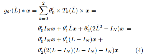
由于切比雪夫多项式具有最佳一致逼近的特性, 在拟合谱图滤波器实现谱图卷积时, 具有较低的拟合误差, 同时避免了对拉普拉斯矩阵的谱分解, 大大降低了计算复杂度. 另外, 一阶GCN节点的邻域组成较为简单, 每次提取节点特征时只考虑到直接相连的邻居节点信息, 而忽视了非直接相连的邻域信息, 因此本文在构造卷积核时, 使用切比雪夫递推式构造二阶截断展开多项式作为设计二阶近似谱图卷积模块的基础, 基础卷积模块为
$$ \begin{split} {g_{\theta {'}}}(\tilde L) * {{{x}}} =\,&\sum\limits_{k=0}^2 {{\theta '_0} \times {T_k}(\tilde L)} \times {{{x}}}=\\ &{{\theta '_0}}{I_N}{{{x}}} + {\theta '_1}\tilde L{{{x}}} + {\theta '_2}(2{{\tilde L}^2} - {I_N}){{{x}}}\,=\\ &{\theta '_0}{I_N}{{{x}}} + {\theta '_1}{\rm{(}}L - {I_N}{\rm{)}}{{{x}}}\;+\\ & {\theta '_2}(2(L - {I_N})(L - {I_N}) - {I_N}){{{x}}} \end{split} $$ (4) 其中,
$ {{{x}}}\in {{\bf{R}}^N} $ 为图信号,$ {\theta '_0} $ ,$ {\theta '_1} $ ,$ {\theta '_2} $ 为模型参数,${{\tilde L}}=L-{I_N}$ 为调整范围后的拉普拉斯矩阵.为了限制模型参数的数量, 减少过拟合, 我们对基础卷积模块的参数个数进行约简, 一方面考虑到不同阶邻居节点对中心节点具有不同影响作用; 另一方面希望后面能进一步对卷积模块作因式分解约简, 使模型更简单有效, 我们令
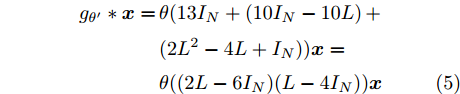
$\theta \!=\!\dfrac{1}{{13}}{\theta '_0}\!=\! - \dfrac{1}{{10}}{\theta '_1}\!=\!{\theta '_2},$ 得到$$ \begin{split} {g_{\theta '}} * {{{x}}} =\,&\theta (13{I_N} + (10{I_N} - 10L)\, +\\ & (2{L^2} - 4L + {I_N})){{{x}}}=\\ &\theta ((2L - 6{I_N})(L - 4{I_N})){{{x}}} \end{split} $$ (5) 将标准化的拉普拉斯矩阵
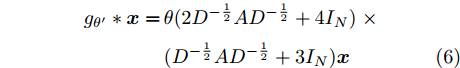
$ L={I_N} - {D^{ - \frac{1}{2}}}A{D^{ - \frac{1}{2}}} $ 代入式(5), 得到$$ \begin{split} {g_{\theta '}} * {{{x}}} =\,&\theta (2{D^{ - \frac{1}{2}}}A{D^{ - \frac{1}{2}}} + 4{I_N})\;\times\\ & ({D^{ - \frac{1}{2}}}A{D^{ - \frac{1}{2}}} + 3{I_N}){{{x}}} \end{split} $$ (6) 由于不同节点边的数量及边的权重幅值不同, 这将会导致边多的(或者边权重幅值大的)节点在聚合后的特征值远远大于边少的(或者边权重幅值小的)节点, 为了消除这一问题, 使构造的卷积模块有助于模型训练时更加稳定有效, 分别对式(6)中的
$ 2{D^{ - \frac{1}{2}}}A{D^{ - \frac{1}{2}}} + 4{I_N} $ 及$ {D^{ - \frac{1}{2}}}A{D^{ - \frac{1}{2}}} + $ $ 3{I_N} $ 两部分进行重新标准化处理并将其表示为$$ 2{D^{ - \frac{1}{2}}}A{D^{ - \frac{1}{2}}} + 4{I_N} \to {\bar D^{ - \frac{1}{2}}}\bar A{\bar D^{ - \frac{1}{2}}} $$ 及其
$$ {D^{ - \frac{1}{2}}}A{D^{ - \frac{1}{2}}} + 3{I_N} \to {{\mathop {D} \limits^ \smallsmile}{} ^{ - \frac{1}{2}}}{\mathop {A} \limits^ \smallsmile} {{\mathop {D} \limits^ \smallsmile}{} ^{ - \frac{1}{2}}} $$ 其中,
${\bar D_{ii}}=\sum\nolimits_j {\bar A}_{ij},$ 且$\bar A=2A + 4{I_N} ;{{\mathop {D} \limits^ \smallsmile} _{ii}}\!=\!\sum\nolimits_j {{{\mathop {A} \limits^ \smallsmile}_{ij}}},$ 且$ {\mathop {A} \limits^ \smallsmile}=A + 3{I_N} $ . 因此得到卷积操作为$$ \begin{array}{l} {g_{\theta '}} * {{{x}}}=\theta ({\bar D^{ - \frac{1}{2}}}\bar A{\bar D^{ - \frac{1}{2}}})({{\mathop {D} \limits^ \smallsmile} {}^{ - \frac{1}{2}}}{\mathop {A} \limits^ \smallsmile} {{\mathop {D} \limits^ \smallsmile}{} ^{ - \frac{1}{2}}}){{{x}}} \end{array} $$ (7) 将该卷积模块推广到具有
$ C $ 个输入通道的信号$ X \in {{\bf{R}}^{N \times C}} $ 和$ F $ 个滤波器上得到最终构造的二阶近似谱图卷积模块为$$ \begin{array}{l} \tilde X=({\bar D^{ - \frac{1}{2}}}\bar A{\bar D^{ - \frac{1}{2}}})({{\mathop {D} \limits^ \smallsmile}{} ^{ - \frac{1}{2}}}{\mathop {A} \limits^ \smallsmile} {{\mathop {D} \limits^ \smallsmile}{} ^{ - \frac{1}{2}}})X{{\Theta }} \end{array} $$ (8) 其中,
$ {{\Theta }} \in {{\bf{R}}^{C \times F}} $ 是一个滤波器参数矩阵,$ \tilde X \in {{\bf{R}}^{N \times F}} $ 表示输入信号卷积之后的结果,$ F $ 为卷积后数据的特征维数. 由式(8)可知, 最终构造的卷积模块在每次更新节点特征表示时能够按照不同权重融合二阶邻域的节点信息, 并且使用重标准化分别对行和列进行归一化处理, 使得模型的训练变得更加稳定有效.1.3 二阶邻域谱图卷积网络前向分层传播过程
为了以端到端的方式将构造的卷积模块用于图节点的分类, 本小节详细阐述二阶邻域谱图卷积网络的前向分层传播过程的实现, 网络输入层的数据
${X_{{\rm{in}}}} \in {{\bf{R}}^{N \times C}}$ 经过隐层(第1个卷积层)卷积运算及非线性激活处理后, 得到节点的隐特征表示${H_{{\rm{out}}}} \in$ $ {{\bf{R}}^{N \times H}} $ , 网络在隐层中的处理过程可以表示为$$ {H_{{\rm{out}}}}=\sigma (\tilde P{X_{{\rm{in}}}}{{{\Theta }}^{\left( 0 \right)}}) $$ (9) 其中,
$\tilde P=({\bar D^{ - \frac{1}{2}}}\bar A{\bar D^{ - \frac{1}{2}}})({{\mathop {D} \limits^ \smallsmile}{} ^{ - \frac{1}{2}}}{\mathop {A} \limits^ \smallsmile} {{\mathop {D} \limits^ \smallsmile}{} ^{ - \frac{1}{2}}}) \in {{\bf{R}}^{N \times N}},$ $ \tilde P $ 为该卷积操作模块的二阶近似卷积算子,$ \sigma \left( \cdot \right) $ 为非线性激活函数, 此处选择ReLU (Rectified linear unit)激活函数用于对数据的非线性化,${{{\Theta }}^{\left( 0 \right)}} \in $ $ {{\bf{R}}^{C \times H}}$ 代表网络在隐层中的可学习权重矩阵, 用于更好地提取节点特征, 其中$ C $ 代表传入该层的输入数据的特征维数,$ H $ 代表数据经过该层卷积及非线性激活后的特征维数.将隐层中得到的节点隐特征表示
${H_{{\rm{out}}}} \in {{\bf{R}}^{N \times H}}$ 送入网络的输出层, 经过输出层的卷积操作及归一化指数函数处理得到每个节点的标签预测结果${O_{{\rm{out}}}} \in {{\bf{R}}^{N \times W}}$ , 网络输出层的处理过程表示为$$ {O_{{\rm{out}}}}={\rm{soft}}\max (\tilde P{H_{{\rm{out}}}}{{{\Theta }}^{\left( 1 \right)}}) $$ (10) 其中,
${\rm{soft}}\max ( \cdot )$ 为归一化指数函数, 用于计算每个节点最终归属于某一类别标签的概率分布, 以此实现对节点的类别标签的预测,$ {{{\Theta }}^{\left( 1 \right)}} \in {{\bf{R}}^{H \times W}} $ 代表网络输出层的可学习权重参数, 其中$ H $ 是每个节点隐特征表示的维数,$ W $ 是数据经过该层卷积及激活操作后的特征维数, 由于该层是网络的输出层, 因此$ W $ 的值设置为与数据集的类别数相等.最终整个谱图卷积网络模型分层传播的过程表示为
$$ {O_{{\rm{out}}}}={\rm{soft}}\max (\tilde P \times \sigma (\tilde P \times {X_{{\rm{in}}}} \times {{{\Theta }}^{\left( 0 \right)}}) \times{{{\Theta }}^{\left( 1 \right)}}) $$ (11) 其中,
$\tilde P=({\bar D^{ - \frac{1}{2}}}\bar A{\bar D^{ - \frac{1}{2}}})({{\mathop {D} \limits^ \smallsmile}{}^ { - \frac{1}{2}}}{\mathop {A} \limits^ \smallsmile} {{\mathop {D} \limits^ \smallsmile} {}^{ - \frac{1}{2}}}) \in {{\bf{R}}^{N \times N}} ,{{{\Theta }}^{\left( 0 \right)}} \in$ $ {{\bf{R}}^{C \times H}} $ ,$ {{{\Theta }}^{\left( 1 \right)}} \in {{\bf{R}}^{H \times W}} $ 为网络的可学习参数矩阵.1.4 二阶邻域谱图卷积网络损失函数设计
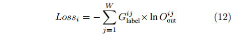
为了引导模型在后向传播过程中对参数的更新, 我们构造交叉熵损失函数来衡量预测数据分布与真实数据分布的差异情况. 将输入数据中的某个有标签的节点数据表示为
$X_{{\rm{in}}}^i \in {{\bf{R}}^C}$ , 则经过模型的前向分层传播过程可得到该节点的预测结果为$O_{{\rm{out}}}^i \!\in\! {{\bf{R}}^W} ,$ 假设该节点真实的类别标签为$G_{{\rm{label}}}^i \!\in \!{{\bf{R}}^W},$ 其中类别标签使用One-Hot编码方式, 则对该节点预测产生的交叉熵损失为$$ Los{s_i}=- \sum\limits_{j=1}^W {G_{{\rm{label}}}^{ij} \times } \ln O_{{\rm{out}}}^{ij} $$ (12) 使用
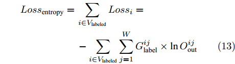
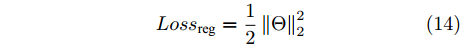
${V_{{\rm{labeled}}}}$ 表示所有给定类别标签的节点数据组成的集合, 则网络对于所有有标签节点数据的交叉熵损失函数为$$ \begin{split} Los{s_{{\rm{entropy}}}} =\,&\sum\limits_{i \in {V_{{\rm{labeled}}}}} {Los{s_i}} =\\ &- \sum\limits_{i \in {V_{{\rm{labeled}}}}} {\sum\limits_{j=1}^W {G_{{\rm{label}}}^{ij} \times \ln O_{{\rm{out}}}^{ij}} } \end{split} $$ (13) 由于模型的复杂度越高, 过拟合的风险也就越大, 因此为了在模型拟合数据能力和模型的复杂度之间取得平衡, 提高模型的泛化性能, 我们在构造损失函数时对模型参数使用
$ {L_2} $ 正则化约束, 并将对模型参数的正则化约束表示为$$ Los{s_{{\rm{reg}}}}=\frac{1}{2}\left\| {{\Theta }} \right\|_2^2 $$ (14) 其中,
$ {{\Theta }} $ 表示模型中的可学习参数,$ {\left\| \cdot \right\|_2} $ 表示矩阵的$ {L_2} $ 范数, 即${\left\| \Theta \right\|_2}=\sqrt {{{\sum\nolimits_i {\sum\nolimits_j {\left( {{\Theta _{ij}}} \right)} } }^2}}$ .最终, 将以上各项结合, 得到模型损失函数为
$$ Los{s_{{\rm{total}}}}=Los{s_{{\rm{entropy}}}} + \omega Los{s_{{\rm{reg}}}} $$ (15) 其中,
$ \omega $ 为超参数, 用于控制正则项大小, 该值越大意味着对模型复杂度的约束越大.2. 实验验证与分析
2.1 实验数据集
本文利用4个公开的标准数据集对模型的有效性进行验证, 具体包括3个引文网络数据集CiteSeer[25], Cora[26], PubMed[27]和1个知识图数据集NELL[28]. 其中CiteSeer数据集主要由计算机相关的科学出版物组成, 包括人工智能、数据库、信息检索及机器语言等相关领域; Cora数据集主要由机器学习相关的论文组成, 涉及到神经网络、遗传算法、概率方法、强化学习等领域; PubMed数据集则主要由生物医学方面的科学出版物构成. 这3个数据集都记录了文献之间的引用及被引用的关系, 并且对于数据集中的每篇文献, 使用去除连接字、标点符号等不能代表文档关键含义的停用词及在文档中出现频率小于10次的词来进行特征描述. NELL(Never ending language learning)数据集是从 NELL知识图[28]中提取出来的数据集, 通过关联选定的NELL实体与ClueWeb09中的文本描述, NELL中的每个关系被描述为一个三元组
$ ({e_h},r,{e_t}), $ 其中$ {e_h} $ 和$ {e_t} $ 分别表示头实体和尾实体,$ r $ 表示两个实体间的关系. 我们遵循文献[2]中的预处理机制, 为每个实体对$ ({e_h},r,{e_t}) $ 分配单独的关系节点$ {r_1} $ 和$ {r_2} $ , 作为$ ({e_h},{r_1}) $ 和$ ({e_t},{r_2}) $ , 以此构成了含有55864个关系节点和9891个实体节点的二分图结构. 另外, 实体节点由5414维稀疏特征向量描述, 通过为每个关系节点分配一个不同的One-Hot向量, 使得每个图节点的特征向量的长度均为5414 + 55864 = 61 278. 4个数据集的详细统计信息见表1.表 1 4个数据集的基本统计信息Table 1 Basic statistics information for four datasets数据集 节点 边 特征 类别 CiteSeer 3327 4732 3703 6 Cora 2708 5429 1433 7 PubMed 19717 44338 500 3 NELL 65755 266144 5414 210 表1中, 对于3个引文网络数据集, 节点表示每个数据集含有科学出版物的总个数, 即图节点的数量; 边表示科学出版物之间的引用与被引用的连接数量, 即图的边数; 特征描述每个出版物特征词的个数, 即图上每个节点的属性信息的维数; 类别代表每一个数据集中包括的出版物的类别数. 对于NELL数据集, 节点表示实体节点与关系节点的总数, 边表示实体节点与关系节点的连接数量, 特征描述每个实体节点的特征词个数, 类别代表数据集中实体节点的类别数.
2.2 实验设置
模型每一层的可学习权值参数按照Glorot & Bengio方式[29]进行初始化, 学习率设为0.01, 并使用Adam优化器[30]对模型参数进行优化, 最大的训练轮次为200, 且当验证集上损失值连续10次的平均值均大于当前损失值时, 模型则自动停止训练. 对于3个引文网络数据集, 隐层节点的个数设置为16, 为了防止过拟合, 设置Dropout rate[31]为0.5,
$ {L_2} $ 正则项系数$ \omega $ 为$ 5 \times {10^{ - 4}} $ , 对于NELL数据集, 隐层节点的个数设置为64, Dropout rate为0.1, 正则项系数$ \omega $ 为$ 1 \times {10^{ - 5}} $ .实验中将本文方法与当前较为经典和流行的方法进行比较, 包括流行正则方法(ManiReg)[6]、半监督嵌入方法(SemiEmb)[7]、深度游动方法(Deep walk)[9]、标签传播方法(Label propagation, LP)[4]、迭代分类算法(ICA)[8]、Planetoid方法(Planetoid)[12]、谱卷积方法(SpectralCNN)[20]、Monet[32]方法、多项式近似卷积的方法(Cheby-Net)[21]以及GCN方法[2].
2.3 客观评价
2.3.1 标准数据集划分下的节点分类结果及分析
本实验中数据集的划分与文献[12]中一致, 对于3个引文网络数据集, 每个类别使用20个有标签节点用于训练, 500个节点用于验证, 1000个节点用于测试. 对于NELL数据集, 每个类别只使用1个有标签节点用于训练, 500个节点用于验证, 969个节点用于测试.
表2中给出了不同方法在不同数据集上的测试结果, 表中数字表示节点分类精度, 所有基准方法的测试结果来自于原论文. 实验结果表明, 本文构造的二阶近似谱图卷积模型在不同数据集上的节点分类任务中的表现均优于其他模型, 这说明在每次更新节点表示时, 通过恰当地融合直接邻域信息和非直接邻域信息能够更加充分地利用到图的结构信息, 从而能够提取到更有效的节点特征表示, 验证了模型对节点分类的有效性. 对于传统的ManiReg、SemiEmd、LP及DeepWalk等方法, 由于不能充分地利用到已知的给定信息(如节点特征信息或者类别标签信息等), 导致分类精度相对较低. 而对于SpectralCNN、Cheby-Net、Monet方法, 由于模型的参数过于冗杂, 容易导致提取到过多的噪声信息使得测试精度下降. GCN方法在每次更新节点特征表示时, 只整合一阶邻居节点的信息而忽略了非直接的邻域结构信息, 导致每次在更新节点特征表示时缺乏丰富的结构信息, 从而降低了分类性能.
表 2 分类准确率结果汇总(%)Table 2 Summary of results in terms of classification accuracy (%)算法 CiteSeer Cora PubMed NELL ManiReg 60.1 59.5 70.7 21.8 SemiEmb 59.6 59.0 71.1 26.7 LP 45.3 68.0 63.0 26.5 DeepWalk 43.2 67.2 65.3 58.1 ICA 69.1 75.1 73.9 23.1 Planetoid 64.7 75.7 77.2 61.9 SpectralCNN 58.9 73.3 73.9 — Cheby-Net 69.8 81.2 74.4 — Monet — 81.7 78.8 — GCN 70.3 81.5 79.0 66.0 本文算法 71.8 82.6 79.8 67.2 2.3.2 低标签率下的节点分类结果及分析
由于真实数据集中的标签率(有标记数据占的比例)通常很低, 因此研究少量标记训练数据下模型的预测性能具有重要意义. 在本小节中, 通过减少训练样本的数量来检验在给定有限数量的标记数据下模型是否仍然表现出良好的分类效果. 具体地, 在实验中对于3个引文网络数据集, 从每个类别中随机选择15, 10, 5个有标签的节点用于模型训练, 随机选择500个节点作为验证集, 1000个节点用于对模型的测试. 为了避免一次随机划分数据带来的偶然性, 在实验中通过20次随机划分数据集对模型进行测试, 并将20次的平均测试结果作为最终的测试精度.
图2 ~ 4中给出了不同方法(MLP, Cheby1, Cheby2, Cheby3, GCN, 本文算法)在不同划分数据集上进行20次实验后节点的平均分类精度(带有标准偏差). 实验结果表明, 在每个数据集上, 随着带标签训练样本个数的减少, 所有模型的分类精度也随之下降, 并且标准差随之增大. 另外可以发现本文提出模型在不同数据集上的不同标签率下均一致性地优于其他模型的测试结果, 且取得了更小的标准差. 这表明在更低标签率下模型也能够表现出更加优越的分类性能, 验证了模型的稳定性.
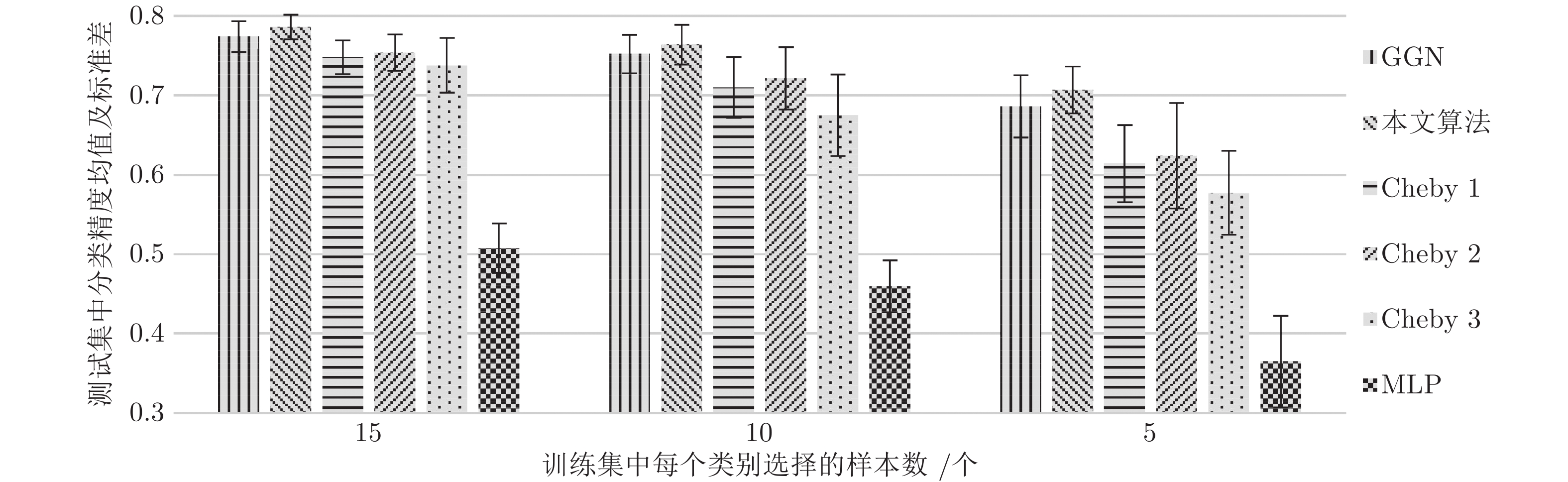 图 2 Cora上不同训练集大小(每个类的标记节点数)的准确率Fig. 2 Accuracy for different training set sizes (number of labeled nodes per class) on Cora
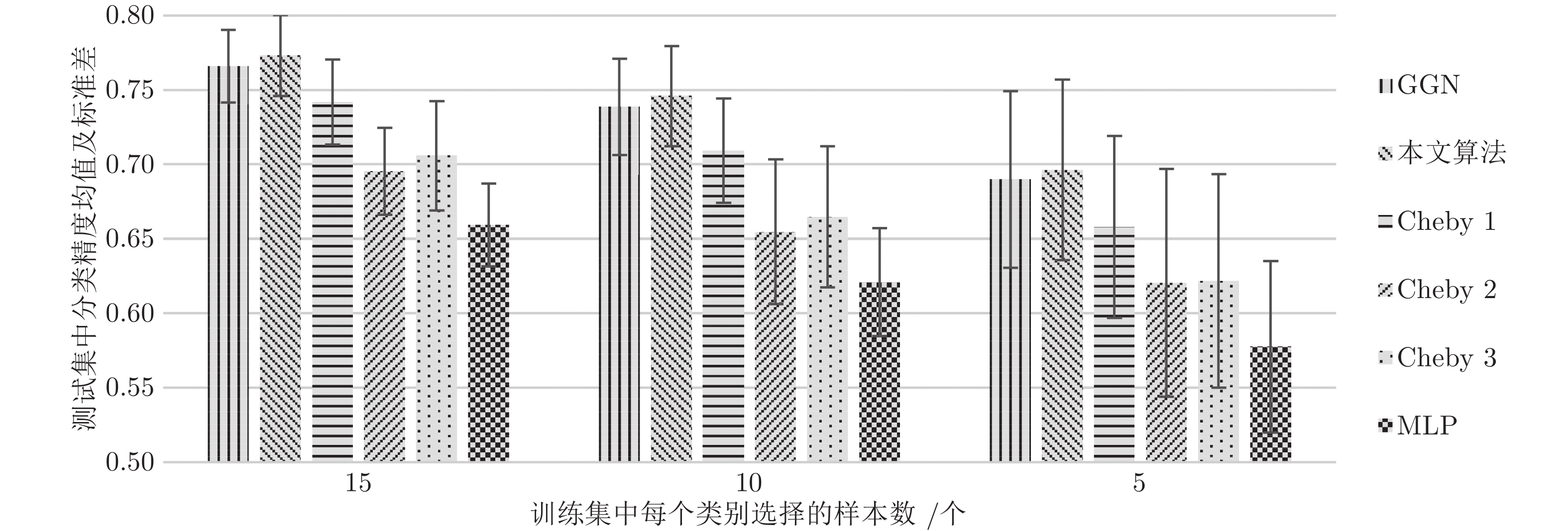 图 4 PubMed上不同训练集大小(每个类的标记节点数)的准确率Fig. 4 Accuracy for different training set sizes (number of labeled nodes per class) on PubMed
 图 3 CiteSeer上不同训练集大小(每个类的标记节点数)的准确率Fig. 3 Accuracy for different training set sizes (number of labeled nodes per class) on CiteSeer
2.3.3 训练模型的计算复杂度分析
我们将本文提出的二阶近似谱图卷积网络模型与一阶GCN模型(GCN)进行比较分析. 具体地, 网络模型的层数均为2, 属性矩阵
$X \in {{\bf{R}}^{N \times C}} ,$ 邻接矩阵使用稀疏矩阵存储, 图中边的个数为$ \left| E \right| $ (图结构添加自环), 顶点个数为$ N $ , 网络第1层得到的特征维数为$ H $ , 网络第2层得到的特征维数为$W$ . 由文献[2]可知, 一阶GCN模型在网络的第1层需要乘法运算次数为$ \left| E \right|H + NCH $ , 网络第2层需要的乘法运算次数为$\left| E \right|W + NHW$ , 共需要乘法运算次数为$\left| E \right| (H + W) + NH(C + W)$ , 模型的计算复杂度为${\rm{O}}(\left| E \right|CHW)$ , 由于CHW均为特征维数, 与问题规模无关, 因此计算复杂度与图中边数呈线性关系. 而本文提出的模型在网络第1层需要乘法运算次数为$ 2\left| E \right|H + NCH $ , 网络的第2层需要乘法运算次数为$2\left| E \right|W + NHW$ , 共需要乘法运算次数为$2\left| E \right|(H + W) + NH(C + W)$ , 模型的计算复杂度为${\rm{O}}(\left| E \right|CHW)$ . 由此可以看出, 本文提出的模型与一阶GCN相比, 在计算复杂度的规模上是相同的, 但是由于本文构造的卷积模块引入了二阶邻居节点的特征信息, 导致相应的增加了一些乘法运算次数.2.4 二阶邻域优势的案例分析
为了更加显式地揭示本文提出的二阶近似谱图卷积模型相比一阶GCN模型[2]的优势, 我们通过案例对模型定性分析. 具体地, 在Cora数据集中随机选择了一个使用本文方法分类正确而使用GCN方法分类错误的节点并记作
$ t $ , 图5(a)绘制了由该节点的一阶邻域组成的局部网络, 图5(b)绘制了由该节点的两阶邻域组成的局部网络. 图中每个节点的值代表它们的真实类别标签, 节点的背景深度代表GCN及本文模型得到的每个节点对目标节点$ t $ 的特征聚合权重, 颜色越深表示权重值越大. 图 5 目标节点t的一阶及两阶邻域组成的局部网络示意图Fig. 5 Schematic diagram of local network composed of the first-order and two-order neighborhoods of target node t
图5(a)展示的情况是对GCN方法分类的一个鲁棒性检测, 这是由于GCN方法预测节点
$ t $ 的标签时, 只利用了$ t $ 的一阶邻居以及自身的信息来进行标签预测, 而在节点$ t $ 的一阶邻居节点中, 类别标签2和5的数量是相同的, 类别标签3的数量最少, 相同标签的节点特征是相近的, 但是自身特征和一阶邻居特征参考的尺度是不同的, GCN方法最终将$ t $ 节点的类别预测为了标签5. 由图5(b)可知, 本文方法通过有效地融合目标节点的二阶邻居信息, 用于增强目标节点的特征表示, 从而正确地预测出了节点$ t $ 的类别标签为3.2.5 节点隐特征表示可视化分析
为了更直观地观测模型提取到的节点特征表示的有效性, 我们使用T-SNE方法[33]对模型在隐层提取到的节点特征表示进行可视化, 如图6所示. 图中不同的数字表示不同的类别标签. 从图中我们不难发现模型提取到的隐特征表示在投影二维空间中均表现出了明显的类簇效果. 具体地, 以图6(a)为例, 图中的这些聚类簇对应了Cora数据集的7个类别标签, 验证了模型对Cora数据集的7个主题类别的区分能力. 同样地, 图6(b)和图6(c)分别表现出了6个和3个主题类别. 说明通过利用丰富的结构信息, 模型在学习过程中提取到了比较有分辨力的节点特征信息.
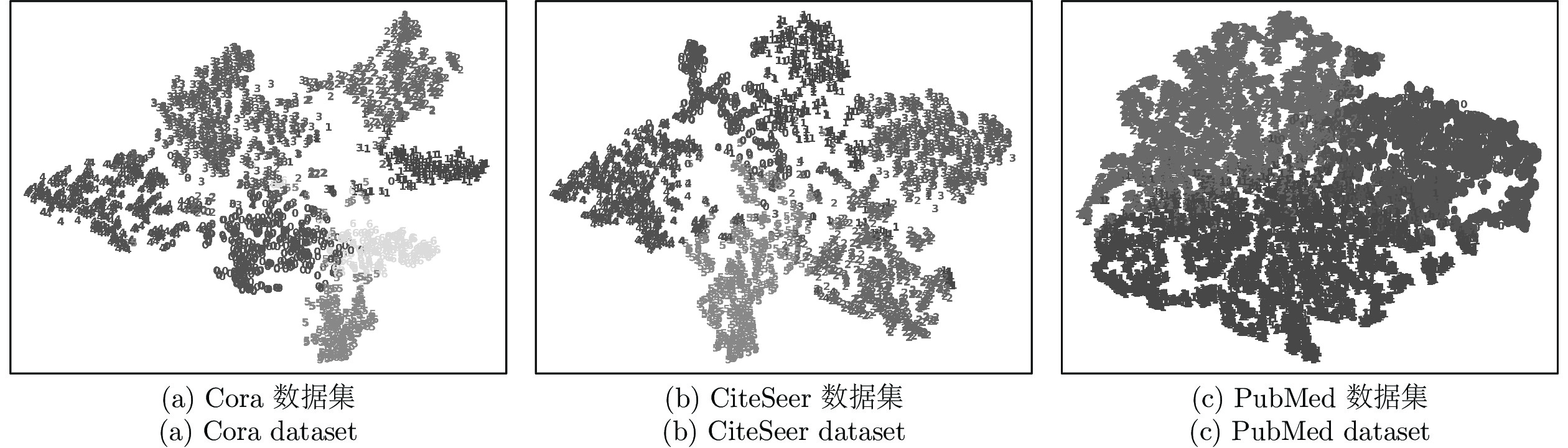 图 6 在3个数据集上模型隐含层学习到的隐特征表示的t-SNE图Fig. 6 A t-SNE plot of the learned hidden feature representations of the model’s hidden layer on the three datasets
综上所述可以看出, 无论在不同数据集上通过节点分类任务进行客观评价, 还是给出的对比案例分析及隐特征表示的可视化效果, 本文的方法均表现出了较好的效果, 验证了模型的有效性.
3. 结论
针对图上半监督节点分类任务, 本文结合切比雪夫截断展开多项式及标准化的拉普拉斯矩阵, 提出了用于谱图卷积网络的二阶近似卷积模块, 首先利用切比雪夫二阶截断展开式构造基础模型, 然后对模型进行参数精简及优化处理, 使其更新节点特征表示时能够更加有效地利用结构信息, 进而获得更具表达力的节点表示, 实现对图上节点的分类. 在公开的标准数据集上进行实验验证, 结果表明在多种标签率下我们的模型分类效果均优于当前流行方法, 验证了本文提出模型的有效性. 但是由于使用本文提出的方法对节点分类时, 需要将整个图结构加载到模型中, 因此很难适用于较大规模的图. 在未来的研究中, 为了使模型更适应于处理较大规模的图, 我们考虑采用首先将图划分成多个小规模的图, 然后分别进行处理的策略进行改进.
-
图 1 本文构造的二阶邻域谱图卷积网络描述图
Fig. 1 A schematic diagram of our two-order neighborhood spectral convolution network
图 2 Cora上不同训练集大小(每个类的标记节点数)的准确率
Fig. 2 Accuracy for different training set sizes (number of labeled nodes per class) on Cora
图 4 PubMed上不同训练集大小(每个类的标记节点数)的准确率
Fig. 4 Accuracy for different training set sizes (number of labeled nodes per class) on PubMed
图 3 CiteSeer上不同训练集大小(每个类的标记节点数)的准确率
Fig. 3 Accuracy for different training set sizes (number of labeled nodes per class) on CiteSeer
图 5 目标节点t的一阶及两阶邻域组成的局部网络示意图
Fig. 5 Schematic diagram of local network composed of the first-order and two-order neighborhoods of target node t
图 6 在3个数据集上模型隐含层学习到的隐特征表示的t-SNE图
Fig. 6 A t-SNE plot of the learned hidden feature representations of the model’s hidden layer on the three datasets
表 1 4个数据集的基本统计信息
Table 1 Basic statistics information for four datasets
数据集 节点 边 特征 类别 CiteSeer 3327 4732 3703 6 Cora 2708 5429 1433 7 PubMed 19717 44338 500 3 NELL 65755 266144 5414 210  下载: 导出CSV
表 2 分类准确率结果汇总(%)
Table 2 Summary of results in terms of classification accuracy (%)
算法 CiteSeer Cora PubMed NELL ManiReg 60.1 59.5 70.7 21.8 SemiEmb 59.6 59.0 71.1 26.7 LP 45.3 68.0 63.0 26.5 DeepWalk 43.2 67.2 65.3 58.1 ICA 69.1 75.1 73.9 23.1 Planetoid 64.7 75.7 77.2 61.9 SpectralCNN 58.9 73.3 73.9 — Cheby-Net 69.8 81.2 74.4 — Monet — 81.7 78.8 — GCN 70.3 81.5 79.0 66.0 本文算法 71.8 82.6 79.8 67.2
下载: 导出CSV
-
[1] Meng Z Q, Liang S S, Bao H Y, Zhang X L. Co-embedding attributed networks. In: Proceedings of the 12th ACM International Conference on Web Search and Data Mining, New York, NY, USA: ACM, 2019. 393−401 [2] Kipf T N, Welling M. Semi-supervised classification with graph convolutional networks. In: Proceedings of the 5th International Conference on Learning Representations, Toulon, France: OpenReview, 2017. 1−14 [3] Liu Z Q, Chen C C, Yang X X, Zhou J, Li X L, Song L. Heterogeneous graph neural networks for malicious account detection. In: Proceedings of the 27th International Conference on Information and Knowledge Management, New York, NY, USA: ACM, 2018. 2077−2085 [4] Zhu X J, Ghahramani Z, Lafferty J D. Semi-supervised learning using Gaussian fields and harmonic functions. In: Proceedings of the 20th International Conference on Machine Learning, Menlo Park, CA, USA: AAAI, 2003. 912−919 [5] Talukdar P P, Crammer K. New regularized algorithms for transductive learning. In: Proceedings of the 2009 European Conference on Machine Learning and Principles and Practice of Knowledge Discovery in Databases, Berlin, Germany: Springer, 2009. 442−457 [6] Belkin M, Niyogi P, Sindhwani V. Manifold regularization: A geometric framework for learning from labeled and unlabeled examples. Journal of Machine Learning Research, 2006, 7(11): 2399−2434 [7] Weston J, Frédéric R, Collobert R. Deep learning via semi-supervised embedding. In: Proceedings of the 25th International Conference on Machine Learning, Berlin, Germany: Springer, 2012. 639−655 [8] Lu Q, Getoor L. Link-based classification. In: Proceedings of the 20th International Conference on Machine Learning, Menlo Park, CA, USA: AAAI, 2003. 496−503 [9] Perozzi B, Al-Rfou R, Skiena S. Deepwalk: Online learning of social representations. In: Proceedings of the 20th ACM SIGKDD International Conference on Knowledge Discovery and Data Mining, New York, NY, USA: ACM, 2014. 701−710 [10] Tang J, Qu M, Wang M Z, Zhang M, Yan J, Mei Q Z. Line: Large-scale information network embedding. In: Proceedings of the 24th International Conference on World Wide Wed, New York, NY, USA: ACM, 2015. 1067−1077 [11] Grover A, Leskovec J. Node2vec: Scalable feature learning for networks. In: Proceedings of the 22nd ACM SIGKDD International Conference on Knowledge Discovery and Data Mining, New York, NY, USA: ACM, 2016. 855−864 [12] Yang Z L, Cohen W W, Salakhutdinov R. Revisiting semi-supervised learning with graph embeddings. In: Proceedings of the 33rd International Conference on Machine Learning, Cambridge, MA, USA: MIT Press, 2016. 40−48 [13] Mikolov T, Sutskever I, Chen K, Corrado G S, Dean J. Distributed representations of words and phrases and their compositionality. In: Proceedings of the 27th Annual Conference on Neural Information Processing Systems, New York, NY, USA: Curran Associates, 2013. 3111−3119 [14] Sun K, Xiao B, Liu D, Wang J D. Deep high-resolution representation learning for human pose estimation. In: Proceedings of the 2019 IEEE Conference on Computer Vision and Pattern Recognition, New York, USA: IEEE, 2019. 5693−5703 [15] Zhang Y, Pezeshki M, Brakel P, Zhang S Z, Laurent C, Bengio Y, et al. Towards end-to end speech recognition with deep convolutional neural networks. In: Proceedings of the 17th Annual Conference of the International Speech Communication Association, New York, USA: Elsevier 2016. 410−414 [16] Niepert M, Ahmed M, Kutzkov K. Learning convolutional neural networks for graphs. In: Proceedings of the 33rd International Conference on Machine Learning, Cambridge, MA, USA: MIT Press, 2016. 2014−2023 [17] Velickovic P, Cucurull G, Casanova A, Romero A, Liò P, Bengio Y. Graph attention networks. In: Proceedings of the 6th International Conference on Learning Representations, Vancouver, BC, Canada: OpenReview, 2018. 1−12 [18] Gao H Y, Wang Z Y, Ji S W. Large-scale learnable graph convolutional networks. In: Proceedings of the 24th ACM SIGKDD International Conference on Knowledge Discovery and Data Mining, New York, NY, USA: ACM, 2018. 1416−1424 [19] Hamilton W L, Ying Z T, Leskovec J. Inductive representation learning on large graphs. In: Proceedings of the 31st Annual Conference on Neural Information Processing Systems, New York, NY, USA: Curran Associates, 2017. 1024−1034 [20] Bruna J, Zaremba W, Szlam A, Lecun Y. Spectral networks and locally connected networks on graphs. In: Proceedngs of the 2nd International Conference on Learning Representations, Banff, AB, Canada: OpenReview, 2014. 1−14 [21] Defferrard M, Bresson X, Vandergheynst P. Convolutional neural networks on graphs with fast localized spectral filtering. In: Proceedings of the 29th Annual Conference on Neural Information Processing Systems, New York, NY, USA: Curran Associates, 2016. 3844−3852 [22] Hammond D K, Vandergheynst P, Rémi G. Wavelets on graphs via spectral graph theory. Applied and Computational Harmonic Analysis, 2012, 30(2): 129−150 [23] Li Q M, Han Z C, Wu X M. Deeper insights into graph convolutional networks for semi-supervised learning. In: Proceedings of the 32nd AAAI Conference on Artificial Intelligence, Menlo Park, CA, USA: AAAI, 2018. 3538−3545 [24] Shuman D I, Narang S K, Frossard P, Ortega A, Vandergheynst P. The emerging field of signal processing on graphs: Extending high-dimensional data analysis to networks and other irregular domains. IEEE Signal Processing Magazine, 2013, 30(3): 83−98 doi: 10.1109/MSP.2012.2235192 [25] Giles C L, Bollacker K, Lawrence S. Citeseer: An automatic citation indexing system. In: Proceedings of the 3rd ACM International Conference on Digital Libraries, New York, NY, USA: ACM, 1998. 89−98 [26] McCallum A, Nigam K, Rennie J, Seymore K. Automating the construction of internet portals with machine learning. Information Retrieval, 2000, 3(2): 127−163 doi: 10.1023/A:1009953814988 [27] Namata G, London B, Getoor L, Huang B. Query-driven active surveying for collective classification. In: Proceedings of the 10th workshop on Mining and Learning with Graphs, Edinburgh, Scotland: ACM, 2012. 1−8 [28] Andrew C, Justin B, Bryan K, Burr S, Estevam R H J, Tom M M. Toward an architecture for never-ending language learning. In: Proceedings of the 24th AAAI Conference on Artificial Intelligence, Menlo Park, CA, USA: AAAI, 2010. 1306−1313 [29] Glorot X, Bengio Y. Understanding the difficulty of training deep feedforward neural networks. In: Proceedings of the 13th International Conference on Artificial Intelligence and Statistics, Cambridge, MA, USA: MIT Press, 2010. 249−256 [30] Kingma D P, Ba J. Adam: A method for stochastic optimization. In: Proceedings of the 3rd International Conference on Learning Representations, San Diego, CA, USA: OpenReview, 2015. 1−15 [31] Srivastava N, Hinton G, Krizhevsky A, Sutskever I, Salakhutdinov R. Dropout: A simple way to prevent neural networks from overfitting. Journal of Machine Learning Research, 2014, 15(1): 1929−1958 [32] Monti F, Boscaini D, Masci J, Rodola E, Svoboda J, Bronstein M M. Geometric deep learning on graphs and manifolds using mixture model CNNs. In: Proceedings of the 2017 IEEE Conference on Computer Vision and Pattern Recognition, New York, USA: IEEE, 2017. 5425−5434 [33] Van der Maaten L, Hinton G. Visualizing data using t-SNE. Journal of Machine Learning Research, 2008, 9(11): 2579−2605 期刊类型引用(1)
1. 李文静,白静,彭斌,杨瞻源. 图卷积神经网络及其在图像识别领域的应用综述. 计算机工程与应用. 2023(22): 15-35 .  百度学术
百度学术其他类型引用(3)
-


 下载:
下载:


计量
- 文章访问数: 838
- HTML全文浏览量: 236
- PDF下载量: 187
- 被引次数: 4
