

Synergistic Path Planning for Multiple Vehicles Based on an Improved Particle Swarm Optimization Method
-
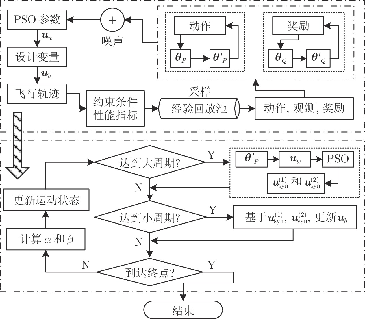
摘要: 考虑气动、轨迹、约束、指标间的耦合关系, 以多高超声速飞行器同时到达为目标建立了协同规划模型; 设计了一种自动满足终端约束的全新滑翔飞行剖面, 减少了规划算法需要处理的约束数量; 推导了滑翔段高精度解析解, 实现了过程约束和性能指标的快速求解; 提出了一种改进粒子群优化(Particle swarm optimization, PSO)算法, 借助强化学习方法构建协同需求与惯性权重间的动态映射网络, 提高了在线规划效率. 最后通过数学仿真验证了方法的正确性和有效性.Abstract: This paper researches the synergistic flight for multiple hypersonic vehicles. The synergistic planning problem is formulated in view of the nonlinear coupling among aerodynamics, the performance index, and the path constraints. Then, the gliding profile, which naturally satisfies the terminal constraints and decreases the constraints, is proposed. Meanwhile, accurate solutions are deduced in the glide phase, so path constraints and the performance index can be quickly derived. An improved particle swarm optimization (PSO) method is developed by building the network between synergistic requirements and the optimal inertial weight in PSO based on a reinforcement learning method. Thus, the efficiency online computational efficiency can be largely improved. Numerical simulation results indicate the efficiency of the proposed method.
-
表 1 初始状态和终端约束
Table 1 The initial states and the terminal constraints
初始值 经纬度 (°) 高度 (km) 速度 (m/s) 飞行路径角 (°) 剩余航程 (km) 飞行器 1 E 90, N 45 56 5400 −2.0 2304 飞行器 2 E 65, N 30 54 5300 −2.0 2263 飞行器 3 E 40, N 35 52 5200 −1.0 2324 飞行器 4 E 70, N 70 50 5100 −1.0 2285 终端值 E 60, N 50 25 — −1.0 0  下载: 导出CSV
表 2 基本PSO和改进PSO计算效率对比
Table 2 Comparison of the computation efficiency
进化代数 最大值 最小值 平均值 标准差 基本 PSO 20 8 14 3.17 改进 PSO 16 6 10 2.69
下载: 导出CSV
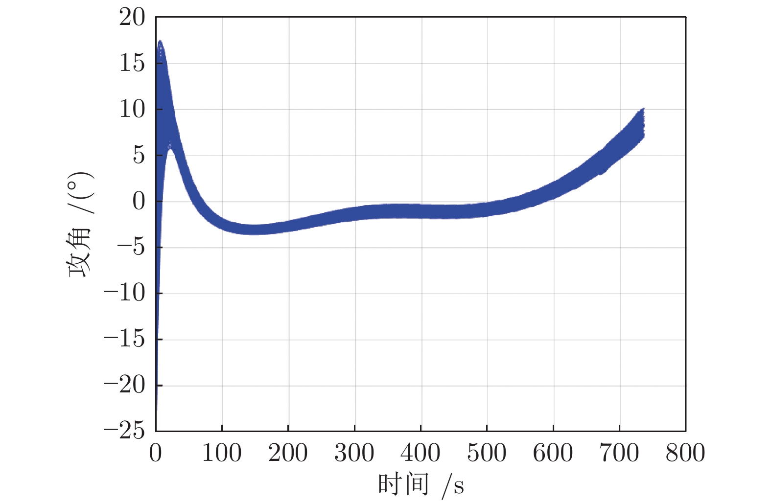
表 3 滑翔段干扰因素设置
Table 3 Disturbances in the glide phase
序号 干扰因素 $3\sigma $值 1 初始速度 (m/s) 30 2 初始飞行路径角 (°) 0.2 3 初始高度 (m) 500 4 初始航向偏差 (°) 0.2 5 初始剩余航程 (km) 50 6 气动系数 (%) 10 7 大气密度 (%) 10
下载: 导出CSV
-
[1] 王颖, 闵昌万, 刘秀明, 刘全军, 王官宇. 类HTV-2飞行器横侧向稳定设计研究. 宇航学报, 2017, 38(6): 583-589.Wang Ying, Min Chang-Wan, Liu Xiu-Ming, Liu Quan-Jun, Wang Guan-Yu. Study on lateral-directional stable design of HTV-2 like vehicle. Journal of Astronautics, 2017, 38(6): 583-589. [2] Li J, He M, Li X P, Zhang C F. Multi-physics modeling of electromagnetic wave-hypersonic vehicle interactions under high-power microwave illumination: 2D case. IEEE Transactions on Antennas and Propagation, 2018, 66(7): 3653-3664. doi: 10.1109/TAP.2018.2835300 [3] Borg M P, Kimmel R. Ground test of transition for Hifire-5b at flight-relevant attitudes. Journal of Spacecraft and Rockets, 2018, 55(6): 1-12. [4] 宋巍, 梁轶, 王艳, 袁成, 王竹溪. 2018年国外高超声速技术发展综述. 飞航导弹, 2019, 5: 7-12.Song Wei, Liang Tie, Wang Yan, Yuan Cheng, Wang Zhu- Xi. Summary of the development of hypersonic technology in 2018. Aerodynamic Missile Journal, 2019, 5: 7-12. [5] 杨金龙, 林旭斌. 日本高速/高超声速导弹计划分析. 飞航导弹, 2019, 409(1): 27-30.Yang Jin-Long, Lin Xu-Bin. Analysis on Japan high-speed/ hypersonic missile plane. Aerodynamic Missile Journal, 2019, 409(1): 27-30. [6] Qu Feng, Sun Di, Zuo Guang. A study of upwind schemes on the laminar hypersonic heating predictions for the reusable space vehicle. Acta Astronautica, 2018, 147: 412-420. doi: 10.1016/j.actaastro.2018.03.046 [7] Jia X, Wu S T, Wen Y M, Yao Z. A distributed decision method for missiles autonomous formation based on potential game. Journal of Systems Engineering and Electronics, 2019, 30(4): 738-748. doi: 10.21629/JSEE.2019.04.11 [8] 孙长银, 穆朝絮, 余瑶. 近空间高超声速飞行器控制的几个科学问题研究. 自动化学报, 2013, 39(11): 1901-1913. doi: 10.3724/SP.J.1004.2013.01901Sun Chang-Yin, Mu Zhao-Xu, Yu Yao. Some control problems for near space hypersonic vehicles. Acta Automatica Sinica, 2013, 39(11): 1901-1913. doi: 10.3724/SP.J.1004.2013.01901 [9] Liao Y X, Li H F, Bao W M. Three-dimensional diving guidance for hypersonic gliding vehicle via integrated design of FTNDO and AMSTSMC. IEEE Transactions on Industrial Electronics, 2018, 65(3): 2704-2715. doi: 10.1109/TIE.2017.2736499 [10] 王芳, 林涛, 张克, 崔乃刚. 多阶段高斯伪谱法在编队最优控制中的应用. 宇航学报, 2015, 36(11): 1262-1269. doi: 10.3873/j.issn.1000-1328.2015.11.007Wang Fang, Lin Tao, Zhang Ke, Cui Nai-Gang. Application of multi-phase Gauss pseudospectral method in optimal control for formation. Journal of Astronautics, 2015, 36(11): 1262-1269. doi: 10.3873/j.issn.1000-1328.2015.11.007 [11] Vincent R, Mohammed T, Gilles L. Fast genetic algorithm path planner for fixed-wing military UAV using GPU. IEEE Transactions on Aerospace and Electronic Systems, 2018, 54(5): 2105-2117. doi: 10.1109/TAES.2018.2807558 [12] Chen Q Y, Lu Y F, Jia G W, Li Y, Zhu B J, Lin J C. Path planning for UAVs formation reconfiguration based on Dubins trajectory. Journal of Central South University, 2018, 25(11): 2664-2676. doi: 10.1007/s11771-018-3944-z [13] Xu X G, Wei Z Y, Ren Z, Li S S. Time-varying fault-tolerant formation tracking based cooperative control and guidance for multiple cruise missile systems under actuator failures and directed topologies. Journal of Systems Engineering and Electronics, 2019, 30(3): 587-600. doi: 10.21629/JSEE.2019.03.16 [14] (王东风, 孟丽. 粒子群优化算法的性能分析和参数选择. 自动化学报, 2016, 42(10): 1552-1561.Wang Dong-Feng, Meng Li. Performance analysis and parameter selection of PSO algorithms. Acta Automatica Sinica, 2016, 42(10): 1552-1561. [15] 吕柏权, 张静静, 李占培, 刘廷章. 基于变换函数与填充函数的模糊粒子群优化算法. 自动化学报, 2018, 44(1): 74-86.Lv Bai-Quan, Zhang Jing-Jing, Li Zhan-Pei, Liu Yan-Zhang. Fuzzy particle swarm optimization based on filled function and transformation function. Acta Automatica Sinica, 2018, 44(1): 74-86. [16] Zeng L, Zhang H B, Zheng W. A three-dimensional predictor corrector entry guidance based on reduced-order motion equations. Aerospace Science and Technology, 2018, 73: 223−231 [17] Li M M, Hu J. An approach and landing guidance design for reusable launch vehicle based on adaptive predictor corrector technique. Aerospace Science and Technology, 2018, 75: 13-23. doi: 10.1016/j.ast.2017.12.037 [18] Bollino K, Ross M, Doman D. Optimal nonlinear feedback guidance for reentry vehicles. In: Proceedings of the 2016 AIAA Guidance, Navigation and Control Conference and Exhibit. Keystone, USA: AIAA Press, 2006. [19] Garg H. A hybrid PSO-GA algorithm for constrained optimization problems. Applied Mathematics and Computation, 2016, 274: 292-305. doi: 10.1016/j.amc.2015.11.001 -

 下载:
下载:


图(7) / 表(3)
计量
- 文章访问数: 2112
- HTML全文浏览量: 714
- PDF下载量: 547
- 被引次数: 0
