

Hierarchical Monitoring for Multi-unit Chemical Processes Based on Local-global Correlation Features
-
摘要: 针对一类多单元化工过程的监测问题, 提出基于局部−整体相关特征的分层故障检测与故障定位方法, 通过表征单元内部变量相关性、单元与单元间相关性、局部单元与过程整体相关性, 对过程运行状态进行判断, 以提升过程监测的准确性与可靠性. 首先, 采用典型相关分析, 通过引入邻域单元相关变量提取每个单元的独有特征和外部相关特征; 其次, 对每个单元的独有特征和所有单元的外部相关特征建立统计模型实现分层故障检测; 然后, 建立单元−变量分层贡献图, 对故障单元以及故障变量实现分层定位. 通过在Tennessee Eastman仿真过程和一个实验室级甘油精馏过程中的应用说明所提分层监测方法的有效性.Abstract: A hierarchical process monitoring method based on local-global correlation features is proposed for a class of multi-unit chemical processes. The process operation status is identified by characterizing the correlation within a local unit, between units, and between the local unit and the whole process, through which the monitoring reliability is enhanced. First, based on canonical correlation analysis, individual characteristics and external correlation characteristics of each unit are extracted by introducing correlated variables from neighboring units; Second, multivariate statistical monitoring models are established for individual characteristics of each unit and external correlation characteristics of all units; Then, the unit-variable hierarchical contribution plot is established to locate the fault units and fault variables hierarchically. The effectiveness of the proposed hierarchical monitoring is demonstrated through applications to the Tennessee Eastman process and a laboratory distillation process.
-
在工业生产和社会生活中, 存在着大量的复杂系统, 如非线性耦合机械系统[1]、超临界机组[2]等. 这些复杂系统线性化时通常包含了不可控模态, 给其控制器设计与分析带来了挑战. 在过去十几年里, 这类称之为高阶非线性系统的自适应控制问题吸引了很多研究者的关注. Lin等在文献[3-4]中提出了一种新的构造性设计框架−增加幂次积分法, 有效解决了高阶非线性系统的镇定与实际跟踪问题. 借助于这一方法, 文献[5-19]研究了不同条件下高阶不确定非线性系统的自适应控制问题, 取得了一系列研究成果. 值得指出的是, 上述绝大多数研究结果都要求系统的幂次信息完全已知. 然而, 在一些实际应用中, 由于控制系统本身与周围环境存在着各种不确定因素, 使得系统的幂次信息可能无法精确获取. 因此, 进一步探讨具有未知幂次的高阶非线性系统的控制器设计是很有意义并值得研究的问题.
针对具有未知幂次的高阶非线性系统, 文献[20-21]采用改进的增加幂次积分法, 分别给出了状态反馈和输出反馈控制算法. 然而, 这些算法没有考虑系统函数的不确定性, 且需要假设系统的幂次上界信息已知. 文献[22]结合增加幂次积分技术和自适应控制方法, 解决了具有未知幂次和不确定参数的高阶非线性系统的自适应控制问题. 最近, 针对一类具有未知时变幂次的高阶非线性系统, 文献[23]利用障碍李雅普诺夫方法给出了满足全状态约束条件的自适应控制方案. 但文献[22-23]所提控制方案仍然要求系统幂次的上界已知. 为去除这一假设条件, 文献[24]采用增加幂次积分技术和逻辑切换方法, 设计了一种全局切换自适应镇定方案. 该方案的不足在于切换控制信号是非光滑的, 可能会引起抖振问题, 从而激发系统中的高频未建模动态. 为此, 文献[25]利用动态增益法, 提出了一种光滑自适应状态反馈控制器, 但这种控制器仅适用于相对阶为2的非线性系统.
基于以上讨论, 本文研究了一类具有未知幂次的高阶不确定非线性系统的自适应跟踪控制问题. 结合积分反推技术和障碍李雅普诺夫函数, 提出了一种新颖的自适应状态反馈控制策略. 本文所得到的控制策略具有如下优点: 1) 采用对数型障碍李雅普诺夫函数[26-27]解决了系统幂次未知与模型不确定带来的技术难题; 2) 所提出的自适应控制策略中没有包含虚拟控制律的导数信息, 避免了积分反推法中的“计算膨胀”问题; 3) 所设计控制器能够确保闭环系统的所有信号一致有界. 最后, 仿真结果验证了本文理论结果的有效性.
本文采用如下符号:
$ {\bf{R}} $ ,${\bf{R}}_{\geq{{0}}}$ ,${\bf{R}}_{ > {{0}}}$ 分别表示实数、非负实数和正实数集合.$ {{\bf{R}}}^n $ 表示$ n $ 维实向量集合.$ {\rm{sign}}(s) $ 表示变量$ s $ 的符号函数. 对任意正常数$ q $ , 定义$ [s]^q = {\rm{sign}}(s)|s|^q $ .${\bf{Q}}_{{\rm{odd}}}^{\ge 1}$ 表示分子和分母都是正奇整数的所有有理数的集合.1. 问题描述与预备知识
1.1 问题描述
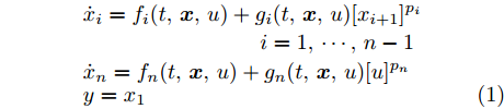
考虑如下高阶不确定非线性系统
$$ \begin{split} & \dot{x}_i = f_i(t,{\boldsymbol{x}},u)+g_i(t,{\boldsymbol{x}},u)[x_{i+1}]^{p_i}\\ &\qquad\qquad\qquad\;\;\;\;\quad i = 1,\cdots,n-1\\ &\dot{x}_n = f_n(t,{\boldsymbol{x}},u)+g_n(t,{\boldsymbol{x}},u)[u]^{p_n}\\& y = x_1 \end{split} $$ (1) 其中,
${\boldsymbol{x}} = [x_1,\cdots,x_n]^{\rm{T}}\in {{\bf{R}}}^n$ 是系统的状态向量, 初始值${\boldsymbol{x}}(0) = [x_1(0),\cdots,x_n(0)]^{\rm{T}}$ ,$\bar{{\boldsymbol{x}}}_i = [x_1,\cdots,x_i]^{\rm{T}}\in {{\bf{R}}}^i$ ,$i = 1,\cdots,n$ ;$ u \in {{\bf{R}}} $ 和$ y \in {{\bf{R}}} $ 分别是控制输入和系统输出;$ p_i\in {\bf{Q}}_{{\rm{odd}}}^{\ge 1} $ ,$i = 1,\cdots,n$ 是系统(1)的未知幂次. 系统函数$ f_i, g_i:{{\bf{R}}}_{\ge0}\times {{\bf{R}}}^n\times {{\bf{R}}}\rightarrow {{\bf{R}}} $ ,$i = 1,\cdots,n$ 在$ t $ 上分段连续, 且关于$ {\boldsymbol{x}} $ 和$ u $ 满足局部Lipschitz条件. 本文的控制目标是设计自适应控制器$ u $ , 使得系统输出$ y $ 跟踪期望轨迹$ y_r $ , 同时确保闭环系统的所有信号皆有界.注 1. 不同于文献[20-25]中的研究结果, 本文中系统幂次无需满足
$ p_1\ge p_2\ge \cdots\ge p_n $ .假设 1. 存在未知的连续函数
$\bar{f}_{il}(\bar{{\boldsymbol{x}}}_i) : {{\bf{R}}}^{i}\rightarrow {{\bf{R}}}_{\geq0}$ ,$ \underline{g}_i(\bar{{\boldsymbol{x}}}_i): {{\bf{R}}}^{i}\rightarrow {{\bf{R}}}_{>0} $ 和$ \bar{g}_i(\bar{{\boldsymbol{x}}}_i): {{\bf{R}}}^{i}\rightarrow {{\bf{R}}}_{>0} $ , 满足$$ |f_i(t,{\boldsymbol{x}},u)|\le \sum\limits_{l = 1}^{j_i}|x_{i+1}|^{q_{il}}\bar{f}_{il}(\bar{{\boldsymbol{x}}}_i) $$ (2) $$ 0<\underline{g}_i(\bar{{\boldsymbol{x}}}_i)\le g_i(t,{\boldsymbol{x}},u)\le \bar{g}_i(\bar{{\boldsymbol{x}}}_i) $$ (3) 其中,
$i = 1,\cdots,n$ ,$l = 1,\cdots,j_i$ ,$ j_i $ 为有限正整数,$ q_{il} $ 为满足$ 0\le q_{i1}<q_{i2}<\cdots<q_{ij_i}<p_i $ 的正常数.注 2. 假设1表明了本文所提控制算法无需知晓系统函数
$ g_i(t,{\boldsymbol{x}},u) $ ,$ f_i(t,{\boldsymbol{x}},u) $ 及相应的界函数$ \underline{g}_i(\bar{{\boldsymbol{x}}}_{i}) $ ,$ \bar{g}_i(\bar{{\boldsymbol{x}}}_{i}) $ ,$ \bar{f}_{il}(\bar{{\boldsymbol{x}}}_i) $ 的解析表达式.假设 2. 期望轨迹
$ y_r $ 为连续可微函数, 且存在未知正常数$ B_r $ , 满足$$ |y_r(t)|+|\dot{y}_r(t)|\le B_r,t\ge 0 $$ (4) 1.2 预备知识
引理 1[28]. 考虑初值问题
$$ \dot{\boldsymbol{\eta}}_r(t) = h_r(t,{\boldsymbol{\eta}}_r),\; {\boldsymbol{\eta}}_r(0) = {\boldsymbol{\eta}}^0_r\in \Xi_r $$ (5) 其中,
$h_r:{{\bf{R}}}_{\ge0}\times \Xi_r\rightarrow {{\bf{R}}}^{{N}}$ 在$ t $ 上分段连续, 且关于$ {\boldsymbol{\eta}}_r $ 满足局部Lipschitz条件,$\Xi_r\subset {{\bf{R}}}^{{N}}$ 为非空开子集.$ {\boldsymbol{\eta}}_r(t) $ 是初值问题(5)在最大存在区间$ [0,t'_f) $ 上的解,$ t'_f<+\infty $ . 设$ \Xi'_r $ 是$ \Xi_r $ 的紧子集, 则存在$t_s\in [0,t'_f)$ , 使得$ {\boldsymbol{\eta}}_r(t_s)\not\in\Xi'_r $ .引理 2[29]. 对任意
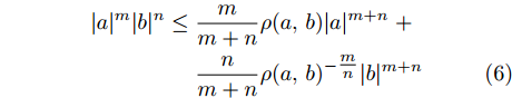
$ a\in {{\bf{R}}} $ ,$ b \in {{\bf{R}}} $ ,$ m\in {{\bf{R}}}_{>0} $ ,$ n\in {{\bf{R}}}_{>0} $ 和函数$ \rho(a,b)>0 $ , 下列不等式成立$$\begin{split} |a|^m|b|^n \le\;& \frac{m}{m+n}\rho(a,b)|a|^{m+n}\;+\\&\frac{n}{m+n}\rho(a,b)^{-\tfrac{m}{n}}|b|^{m+n} \end{split}$$ (6) 引理 3[29-30]. 对任意
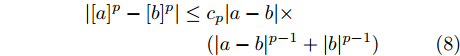
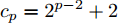
$ p\ge 1 $ ,$ a\in {{\bf{R}}} $ ,$ b \in {{\bf{R}}} $ , 下列不等式成立$$ \|a|^{p}-|b|^{p}|\le |[a]^{p}-[b]^{p}| \hspace{37pt} $$ (7) $$ \begin{split} \,|[a]^{p}-[b]^{p}|\le\; &c_{p}|a-b|\times\\ &(|a-b|^{{p}-1}+|b|^{{p}-1}) \end{split} $$ (8) $$ |a|^{p}+|b|^{p}\le(|a|+|b|)^{p} \hspace{45pt}$$ (9) 其中,
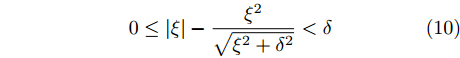
$ c_{p} = 2^{p-2}+2 $ .引理 4[31]. 对任意
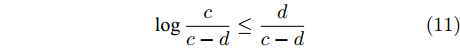
$ \delta\in {{\bf{R}}}_{>0} $ 和$ \xi \in {{\bf{R}}} $ , 下列不等式成立$$ 0\le |\xi|-\frac{\xi^2}{\sqrt{\xi^2+\delta^2}}<\delta $$ (10) 引理 5[32]. 对满足
$ 0\le d<c $ 的$ c\in {{\bf{R}}} $ 和$ d\in {{\bf{R}}} $ , 下列不等式成立$$ \log\frac{c}{c-d} \le \frac{d}{c-d} $$ (11) 2. 自适应跟踪控制策略
本节设计了一种基于障碍李雅普诺夫函数的自适应跟踪控制器, 并给出了闭环系统的稳定性证明.
2.1 自适应控制器设计
定义如下误差坐标变换
$$ z_1 = x_1-y_r $$ (12) $$ z_i = x_i-\alpha_{i-1},\;i = 2,\cdots,n $$ (13) 其中,
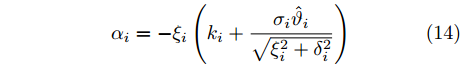
$ \alpha_{i-1} $ 是第$ i-1 $ 步的虚拟控制律.步骤
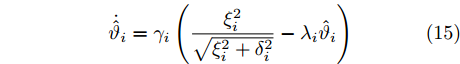
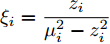
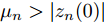
$ {\boldsymbol{i}} $ ${\boldsymbol{(i = 1,\cdots,n-1)}}$ . 选取正常数$ \mu_i $ 满足$ \mu_i>|z_i(0)| $ , 设计第$ i $ 步虚拟控制律和自适应律为$$ \alpha_i = -\xi_i\left(k_i+\frac{\sigma_i\hat{\vartheta}_i}{\sqrt{\xi_i^2+\delta_i^2}}\right) $$ (14) $$ \dot{\hat{\vartheta}}_i = \gamma_i\left(\frac{\xi_i^2}{\sqrt{\xi_i^2+\delta_i^2}}-\lambda_i\hat{\vartheta}_i\right) $$ (15) 其中,
$\xi_i = \dfrac{z_i}{\mu_i^2-z_i^{2}}$ ,$ \hat{\vartheta}_i $ 是$ \vartheta_i $ 的估计值,$ \hat{\vartheta}_i(0)\ge 0 $ ,$ k_i $ ,$ \sigma_i $ ,$ \gamma_i $ 和$ \lambda_i $ 为正常数.步骤 n. 选取正常数
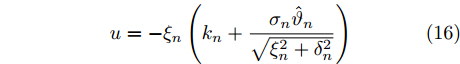
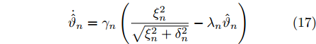
$ \mu_n $ 满足$ \mu_n>|z_n(0)| $ , 设计实际控制律和自适应律为$$ u = -\xi_n\left(k_n+\frac{\sigma_n\hat{\vartheta}_n}{\sqrt{\xi_n^2+\delta_n^2}}\right) $$ (16) $$ \dot{\hat{\vartheta}}_n = \gamma_n\left(\frac{\xi_n^2}{\sqrt{\xi_n^2+\delta_n^2}}-\lambda_n\hat{\vartheta}_n\right) $$ (17) 其中,
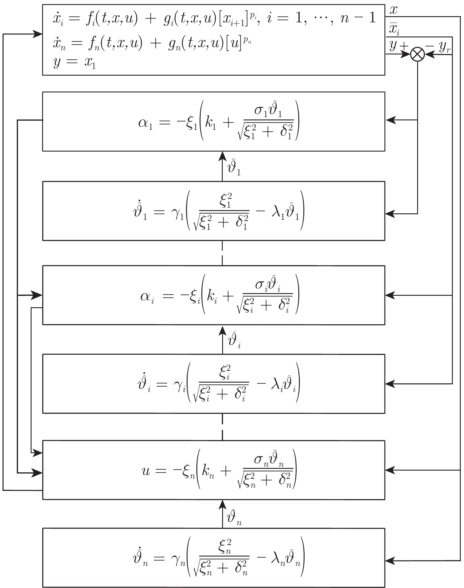
$\xi_n = \dfrac{z_n}{\mu_n^2-z_n^{2}}$ ,$ \hat{\vartheta}_n $ 是$ \vartheta_n $ 的估计值且满足,$\hat{\vartheta}_n(0)\ge 0$ ,$ k_n $ ,$ \sigma_n $ ,$ \gamma_n $ 和$ \lambda_n $ 为正常数.上述自适应控制器的设计过程如图1所示.
注 3. 如式(14) ~ (17)所示, 本文提出的自适应反推控制策略不依赖于系统幂次
$ p_i $ 及其上界信息, 且无需知晓系统函数$ f_i(t,{\boldsymbol{x}},u) $ ,$ g_i(t,{\boldsymbol{x}},u) $ 及相应的界函数$ \bar{f}_{il}(\bar{{\boldsymbol{x}}}_i) $ ,$ \underline{g}_i(\bar{{\boldsymbol{x}}}_{i}) $ ,$ \bar{g}_i(\bar{{\boldsymbol{x}}}_{i}) $ 的解析表达式. 同时, 该控制策略未包含虚拟控制律$ \alpha_i $ 的导数, 消除了积分反推法中“计算膨胀”问题.2.2 稳定性分析
在给出闭环系统的稳定性分析之前, 先引入如下命题.
命题 1. 对式(14) ~ (17)的
$\hat{\vartheta}_1,\cdots,\hat{\vartheta}_n, \alpha_1,\cdots, \alpha_{n-1}$ 和$ u $ , 下列陈述成立i)
$ \hat{\vartheta}_i(t)\ge 0 $ ,$i = 1,\cdots,n$ .ii)
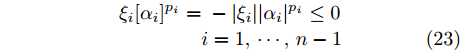
$\xi_i[\alpha_i]^{p_i} = -|\xi_i||\alpha_i|^{p_i} \le 0, \xi_n [u]^{p_n} = -|\xi_n| |u|^{p_n}$ ,$i = 1,\cdots,n-1$ .证明. i) 由于
$\dfrac{\xi_i^2}{\sqrt{\xi_i^2+\delta_i^2}}\ge 0$ 和$ \hat{\vartheta}_i(0)\ge 0 $ , 根据式(15)和式(17), 可直接推出$ \hat{\vartheta}_i(t)\ge 0 $ ,$i = 1,\cdots,n$ .ii) 根据式(14)和式(16),
$ \alpha_i $ ,$i = 1,\cdots,n-1$ 和$ u $ 改写为$$ \alpha_i = \xi_i\phi_i,i = 1,\cdots,n-1 $$ (18) $$ u = \xi_n\phi_n\hspace{74pt} $$ (19) 其中,
$$ \phi_i = -k_i-\frac{\sigma_i\hat{\vartheta}_i}{\sqrt{\xi_i^2+\delta_i^2}},\;\;i = 1,\cdots,n $$ (20) 从而, 有
$$ \begin{split} \xi_i[\alpha_i]^{p_i} =&\; \xi_i|\alpha_i|^{p_i}{\rm{sign}}(\xi_i\phi_i)\\& \quad i = 1,\cdots,n-1\end{split} $$ (21) $$ \xi_n [u]^{p_n} = \xi_n |u|^{p_n}{\rm{sign}}(\xi_n\phi_n) $$ (22) 另外, 由于
$ \hat{\vartheta}_i(t)\ge 0 $ ,$i = 1,\cdots,n$ , 从式(20)易知$ \phi_i\le 0 $ ,$i = 1,\cdots,n$ , 进而可得${\rm{sign}}(\xi_i\phi_i) = -{\rm{sign}}(\xi_i)$ ,$i = 1,\cdots,n$ . 故$$ \begin{split} \xi_i[\alpha_i]^{p_i} =&\; -|\xi_i||\alpha_i|^{p_i}\le 0\\ & i = 1,\cdots,n-1 \end{split}$$ (23) $$ \xi_n [u]^{p_n} = -|\xi_n| |u|^{p_n}\le 0 $$ (24) □
本文主要结论可总结为如下定理.
定理 1. 对满足假设1和假设2的高阶不确定非线性系统(1), 在任意初始条件
$ {\boldsymbol{x}}(0) $ 下, 控制器(16)以及自适应律(15)和(17)保证了闭环系统的所有信号一致有界, 并且输出跟踪误差可以收敛到残差为任意小的残差集.证明. 本证明共分为3部分. 首先, 证明由系统(1), 控制器(16), 自适应律(15)和(17)组成的闭环系统在最大存在区间
$ [0,t_f) $ 上存在唯一解${\pmb\eta}(t) = [z_1(t),\cdots,z_n(t),\hat{\vartheta}_1(t),\cdots,\hat{\vartheta}_n(t)]^{\rm{T}}$ . 然后, 采用反证法证明$ t_f = +\infty $ . 最后, 实现本文控制目标.Part 1. 根据式(14)和式(16), 虚拟控制律
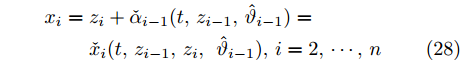
$\alpha_1,\cdots, \alpha_{n-1}$ , 实际控制律$ u $ 以及系统状态$x_1,\cdots,x_n$ 可写为$$ \alpha_i = \check{\alpha}_i(z_i,\hat{\vartheta}_i),i = 1,\cdots,n-1 $$ (25) $$ u = \check{\alpha}_n(z_n,\hat{\vartheta}_n) $$ (26) $$ x_1 = z_1+y_r= \check{x}_1(t,z_1) $$ (27) $$ \begin{split} x_i =\; & z_i+\check{\alpha}_{i-1}(t,z_{i-1},\hat{\vartheta}_{i-1})=\\ & \check{x}_i(t,z_{i-1},z_i,\;\hat{\vartheta}_{i-1}),i = 2,\cdots,n \end{split} $$ (28) 因此, 由式(1)和式(14)
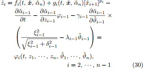
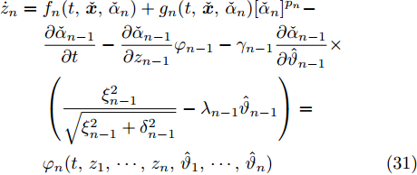
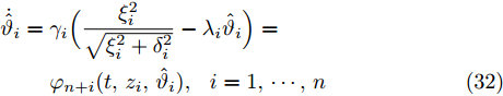
$ \sim $ (17)组成的闭环系统可改写为$$ \begin{split} \dot{z}_1 =\;& f_1(t,\check{{\boldsymbol{x}}},\check{\alpha}_n)+g_1(t,\check{{\boldsymbol{x}}},\check{\alpha}_n)[\check{x}_2]^{p_1}-\dot{y}_r=\\ &\varphi_1(t,z_1,\cdots,z_n,\hat{\vartheta}_1,\cdots,\hat{\vartheta}_n) \end{split} $$ (29) $$ \begin{split} \dot{z}_i = \;& f_i(t,\check{{\boldsymbol{x}}},\check{\alpha}_n)+g_i(t,\check{{\boldsymbol{x}}},\check{\alpha}_n)[\check{x}_{i+1}]^{p_i}\;-\\ &\frac{\partial \check{\alpha}_{i-1}}{\partial t}-\frac{\partial \check{\alpha}_{i-1}}{\partial z_{i-1}}\varphi_{i-1}-\gamma_{i-1}\frac{\partial \check{\alpha}_{i-1}}{\partial \hat{\vartheta}_{i-1}}\;\times\\ &\left(\frac{\xi_{i-1}^2}{\sqrt{\xi_{i-1}^2+\delta_{i-1}^2}}-\lambda_{i-1}\hat{\vartheta}_{i-1}\right)=\\ & \varphi_i(t,z_1,\cdots,z_n,\hat{\vartheta}_1,\cdots,\hat{\vartheta}_n),\\ &\qquad\qquad\qquad\qquad\;\; i = 2,\cdots,n-1 \end{split}$$ (30) $$ \begin{split} \dot{z}_n =\; &f_n(t,\check{{\boldsymbol{x}}},\check{\alpha}_n)+g_n(t,\check{{\boldsymbol{x}}},\check{\alpha}_n)[\check{\alpha}_n]^{p_n}-\\ &\frac{\partial \check{\alpha}_{n-1}}{\partial t}-\frac{\partial \check{\alpha}_{n-1}}{\partial z_{n-1}}\varphi_{n-1}-\gamma_{n-1}\frac{\partial \check{\alpha}_{n-1}}{\partial \hat{\vartheta}_{n-1}}\times\\ &\left(\frac{\xi_{n-1}^2}{\sqrt{\xi_{n-1}^2+\delta_{n-1}^2}}-\lambda_{n-1}\hat{\vartheta}_{n-1}\right)=\\& \varphi_n(t,z_1,\cdots,z_n,\hat{\vartheta}_1,\cdots,\hat{\vartheta}_n) \end{split}$$ (31) $$ \begin{split} \dot{\hat{\vartheta}}_i =\;& \gamma_i\Big(\frac{\xi_i^2}{\sqrt{\xi_i^2+\delta_i^2}}-\lambda_i\hat{\vartheta}_i\Big)=\\ & \varphi_{n+i}(t,z_i,\hat{\vartheta}_i),\;\;i = 1,\cdots,n \end{split} $$ (32) 其中,
$\check{{\boldsymbol{x}}} = [\check{x}_1,\cdots,\check{x}_n]^{\rm{T}}\in {{\bf{R}}}^n$ .定义开集
$$ \Xi = \underbrace{(-\mu_1,\mu_1)\times\cdots\times(-\mu_n,\mu_n)}_n\times {{\bf{R}}}^n $$ 由于
$\mu_i > |z_i(0)|$ ,$i = 1,\cdots,n$ , 可知${\boldsymbol{\eta}}(0) = [z_1(0), \cdots, z_n(0),\hat{\vartheta}_1(0),\cdots,\hat{\vartheta}_n(0)]^{\rm{T}}\in \Xi$ . 同时, 由于期望参考信号$ y_r $ 及其导数$ \dot{y}_r $ 有界, 函数$ f_i, g_i $ ,$i = 1,\cdots, n$ 在$ t $ 上分段连续, 且关于$ {\boldsymbol{x}} $ 和$ u $ 满足局部Lipschitz条件, 可推得$ \varphi_i:{{\bf{R}}}_{\ge0}\times \Xi\rightarrow {{\bf{R}}} $ 在$ t $ 上分段连续, 且关于$ {\boldsymbol{x}} $ 和$ u $ 满足局部Lipschitz条件. 根据微分方程解的存在唯一性定理[33], 对任意初始条件$ {\boldsymbol{\eta}}(0) $ , 闭环系统(29) ~ (32)在最大存在区间$ [0,t_f) $ 上存在唯一解${\boldsymbol{\eta}} = [z_1,\cdots,z_n,\hat{\vartheta}_1,\cdots,\hat{\vartheta}_n]^{\rm{T}}\in \Xi$ , 即, 对$\forall t\in [0,t_f)$ ,$ |z_i|<\mu_i $ ,$i = 1,\cdots,n$ .Part 2. 本部分采用反证法证明
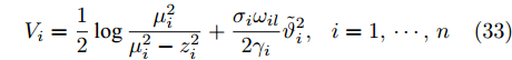
$ t_f = +\infty $ . 为此, 不妨假设$ t_f<+\infty $ .考虑如下障碍李雅普诺夫函数[26]:
$$ V_i = \frac{1}{{2}}\log\frac{\mu_i^2}{\mu_i^2-z_i^{2}}+\frac{\sigma_i\omega_{il} }{2\gamma_i}\tilde{\vartheta}_i^2,\;\;i = 1,\cdots,n $$ (33) 其中,
$ \tilde{\vartheta}_i = \vartheta_i-\hat{\vartheta}_i $ ,$ \omega_{il} $ 是未知正常数.步骤
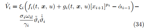
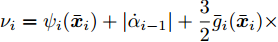
$ {\boldsymbol{i}} $ ${\boldsymbol{(i = 1,\cdots,n-1)}}$ .$ V_i $ 的导数为$$ \begin{split} \dot{V}_i = \;&\xi_i\Big(f_i(t,{\boldsymbol{x}},u)+g_i(t,{\boldsymbol{x}},u)[x_{i+1}]^{p_i}-\dot{\alpha}_{i-1}\Big)-\\ &\frac{\sigma_i\omega_{il} }{\gamma_i}\tilde{\vartheta}_i\dot{\hat{\vartheta}}_i \\[-10pt]\end{split}$$ (34) 其中,
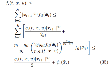
$ \alpha_0 = y_r $ .根据假设1和引理2, 下列不等式成立
$$ \begin{split} &|f_i(t,{\boldsymbol{x}},u)|\le\\ &\qquad\sum\limits_{l = 1}^{j_i}|x_{i+1}|^{q_{il}}\bar{f}_{il}(\bar{{\boldsymbol{x}}}_i)\le\\ &\qquad\sum\limits_{l = 1}^{j_i}\Bigg[\frac{g_i(t,{\boldsymbol{x}},u)|x_{i+1}|^{p_i}}{2j_i}+\\ &\qquad\frac{p_i-q_{il}}{p_i}\left(\frac{2j_iq_{il}\bar{f}_{il}(\bar{{\boldsymbol{x}}}_i)}{p_ig_i(t,{\boldsymbol{x}},u)}\right)^{\frac{q_{il}}{p_i-q_{il}}}\bar{f}_{il}(\bar{{\boldsymbol{x}}}_i)\Bigg]\le\\ &\qquad\frac{g_i(t,{\boldsymbol{x}},u)|x_{i+1}|^{p_i}}{2}+\psi_i(\bar{{\boldsymbol{x}}}_i) \end{split} $$ (35) 其中,
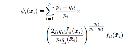
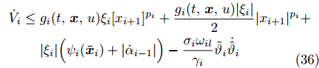
$$ \begin{split} \psi_i(\bar{{\boldsymbol{x}}}_i) =& \sum\limits_{l = 1}^{j_i}\frac{p_i-q_{il}}{p_i}\times\\ &\left(\frac{2j_iq_{il}\bar{f}_{il}(\bar{{\boldsymbol{x}}}_i)}{p_i\underline{g}_i(\bar{{\boldsymbol{x}}}_i)}\right)^{\tfrac{q_{il}}{p_i-q_{il}}}\bar{f}_{il}(\bar{{\boldsymbol{x}}}_i) \end{split}$$ 将式(35)代入式(34), 可得
$$ \begin{split} \dot{V}_i\le\; &g_i(t,{\boldsymbol{x}},u)\xi_i [x_{i+1}]^{p_i}+\frac{g_i(t,{\boldsymbol{x}},u)|\xi_i|}{2}|x_{i+1}|^{p_i}+\\& |\xi_i|\Big(\psi_i(\bar{{\boldsymbol{x}}}_i)+|\dot{\alpha}_{i-1}|\Big)-\frac{\sigma_i\omega_{il} }{\gamma_i}\tilde{\vartheta}_i\dot{\hat{\vartheta}}_i \\[-10pt]\end{split}$$ (36) 根据命题1, 可得
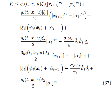
$$ \begin{split} \dot{V}_i\le \;&g_i(t,{\boldsymbol{x}},u)\xi_{i}([x_{i+1}]^{p_i}-[\alpha_{i}]^{p_i})+\\ &\frac{g_i(t,{\boldsymbol{x}},u)|\xi_i|}{2}\Big(|x_{i+1}|^{p_i}-|\alpha_{i}|^{p_i}\Big)+\\ &|\xi_i|\Big(\psi_i(\bar{{\boldsymbol{x}}}_i)+|\dot{\alpha}_{i-1}|\Big)+\\ &\frac{g_i(t,{\boldsymbol{x}},u)\xi_{i}}{2}[\alpha_i]^{p_i}-\frac{\sigma_i\omega_{il} }{\gamma_i}\tilde{\vartheta}_i\dot{\hat{\vartheta}}_i\le\\ &\frac{3g_i(t,{\boldsymbol{x}},u)|\xi_i|}{2}|[x_{i+1}]^{p_i}-[\alpha_{i}]^{p_i}|+\\ &|\xi_i|\Big(\psi_i(\bar{{\boldsymbol{x}}}_i)+|\dot{\alpha}_{i-1}|\Big)-\frac{\sigma_i\omega_{il} }{\gamma_i}\tilde{\vartheta}_i\dot{\hat{\vartheta}}_i+\\& \frac{g_i(t,{\boldsymbol{x}},u)\xi_{i}}{2}[\alpha_i]^{p_i} \end{split}$$ (37) 为了处理式(37)中的项
$ |\xi_i||[x_{i+1}]^{p_i}-[\alpha_{i}]^{p_i}| $ , 考虑以下两种情形.情形 1. 当
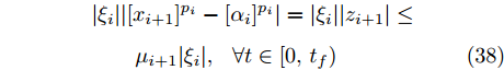
$ p_i = 1 $ 时. 由Part 1可得:$|z_{i+1}| < \mu_{i+1}$ ,$ \forall t\in [0,t_f) $ , 因而$$ \begin{split} &|\xi_i||[x_{i+1}]^{p_i}-[\alpha_{i}]^{p_i}|= |\xi_i||z_{i+1}|\le\\ &\qquad \mu_{i+1}|\xi_i|, \;\;\forall t\in [0,t_f) \end{split} $$ (38) 情形 2. 当
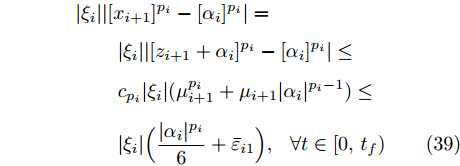
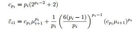
$ p_i>1 $ 时. 由引理2和引理3以及$|z_{i+1}| < \mu_{i+1}$ ,$ \forall t\in [0,t_f) $ , 可得$$\begin{split} &|\xi_i||[x_{i+1}]^{p_i}-[\alpha_{i}]^{p_i}|=\\ &\quad\; \; \; \; |\xi_i||[z_{i+1}+\alpha_{i}]^{p_i}-[\alpha_{i}]^{p_i}|\le\\ &\quad\; \; \; \; c_{p_i}|\xi_i|(\mu_{i+1}^{p_i}+\mu_{i+1}|\alpha_i|^{p_i-1})\le\\ &\quad\; \; \; \; |\xi_i|\Big(\frac{|\alpha_i|^{p_i}}{6}+\bar{\varepsilon}_{i1}\Big),\;\;\forall t\in [0,t_f) \end{split}$$ (39) 其中,
$$ \begin{split} &c_{p_i} = p_i(2^{p_i-2}+2)\\ &\bar{\varepsilon}_{i1} = c_{p_i}\mu_{i+1}^{p_i}+\frac{1}{p_i}\left(\frac{6(p_i-1)}{p_i}\right)^{p_i-1}(c_{p_i}\mu_{i+1})^{p_i} \end{split}$$ 综合情形1和情形2, 项
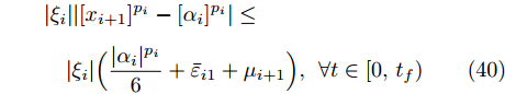
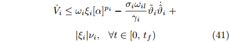
$ |\xi_i||[x_{i+1}]^{p_i}-[\alpha_{i}]^{p_i}| $ 放缩为$$ \begin{split} &|\xi_i||[x_{i+1}]^{p_i}-[\alpha_{i}]^{p_i}| \le\\ &\quad|\xi_i|\Big(\frac{|\alpha_i|^{p_i}}{6}+\bar{\varepsilon}_{i1}+\mu_{i+1}\Big),\;\forall t\in [0,t_f) \end{split} $$ (40) 将式(40)代入式(37)中, 并结合命题1, 易得
$$ \begin{split} \dot{V}_i\le\;&\omega_i\xi_{i}[\alpha]^{p_i}-\frac{\sigma_i\omega_{il} }{\gamma_i}\tilde{\vartheta}_i\dot{\hat{\vartheta}}_i\;+\\ &|\xi_i|\nu_i,\;\;\forall t\in [0,t_f) \end{split} $$ (41) 其中,
$\omega_i = \dfrac{\underline{g}_i(\bar{{\boldsymbol{x}}}_i)}{4}$ ,$\nu_i = \psi_i(\bar{{\boldsymbol{x}}}_i)+|\dot{\alpha}_{i-1}|+\dfrac{3}{2}\bar{g}_i(\bar{{\boldsymbol{x}}}_{i})\times (\bar{\varepsilon}_{i1}+ \mu_{i+1})$ .由Part 1可知, 对
$ \forall t\in [0,t_f) $ ,$ |z_j|<\mu_j $ ,$j = 1, \cdots, i$ . 同时, 依据假设1和假设2,$ y_r $ ,$ \dot{y}_r $ 有界, 且$ \bar{f}_{il} $ ,$ \underline{g}_i $ 和$ \bar{g}_i $ 为连续函数. 此外, 根据第$ i-1 $ 步设计, 可推知$x_1,\cdots,x_i$ ,$ \dot{\alpha}_{i-1} $ 有界,$ \forall t\in [0,t_f) $ . 因此, 运用极值定理, 对$ \forall t\in [0,t_f) $ , 有$$ 0< \omega_{il}\le \omega_i \, $$ (42) $$ 0\le \nu_i\le \nu_{im} $$ (43) 其中,
$ \omega_{il} $ 和$ \nu_{im} $ 为未知正常数.将式(42)和式(43)代入式(41)中, 有
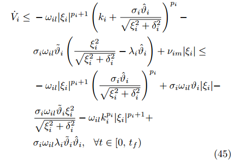
$$ \begin{split} \dot{V}_i\le\;&\omega_{il}\xi_{i}[\alpha_i]^{p_i}-\frac{\sigma_i\omega_{il} }{\gamma_i}\tilde{\vartheta}_i\dot{\hat{\vartheta}}_i+\\ &\nu_{im}|\xi_i|,\;\;\forall t\in [0,t_f) \end{split} $$ (44) 通过式(14)和式(15), 并结合引理3, 可得
$$ \begin{split} \dot{V}_i\le\;&-\omega_{il}|\xi_{i}|^{p_i+1}\left(k_i+\frac{\sigma_i\hat{\vartheta}_i}{\sqrt{\xi_i^2+\delta_i^2}}\right)^{p_i}-\\& \sigma_i\omega_{il} \tilde{\vartheta}_i\left(\frac{\xi_i^2}{\sqrt{\xi_i^2+\delta_i^2}}-\lambda_i\hat{\vartheta}_i\right)+\nu_{im}|\xi_i|\le\\ &-\omega_{il} |\xi_{i}|^{p_i+1}\left(\frac{\sigma_i\hat{\vartheta}_i}{\sqrt{\xi_i^2+\delta_i^2}}\right)^{p_i}+\sigma_i\omega_{il} \vartheta_i|\xi_i|-\\ &\frac{\sigma_i\omega_{il} \tilde{\vartheta}_i\xi_i^2}{\sqrt{\xi_i^2+\delta_i^2}}-\omega_{il} k_i^{p_i}|\xi_{i}|^{p_i+1}+\\ &\sigma_i\omega_{il} \lambda_i\tilde{\vartheta}_i\hat{\vartheta}_i,\;\;\forall t\in [0,t_f) \end{split} $$ (45) 其中,
$\vartheta_i = \dfrac{\nu_{im}}{\sigma_i\omega_{il}}$ .根据引理2和引理4, 式(45)中的项
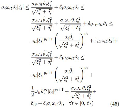
$ \sigma_i\omega_{il}\vartheta_i|\xi_i| $ 放缩为$$ \begin{split} \sigma_i\omega_{il} \vartheta_i|\xi_i|\le\;&\frac{\sigma_i\omega_{il} \vartheta_i\xi_i^2}{\sqrt{\xi_i^2+\delta_i^2}}+\delta_i\sigma_i\omega_{il} \vartheta_i\le\\ &\frac{\sigma_i\omega_{il} \hat{\vartheta}_i\xi_i^2}{\sqrt{\xi_i^2+\delta_i^2}}+\frac{\sigma_i\omega_{il} \tilde{\vartheta_i}\xi_i^2}{\sqrt{\xi_i^2+\delta_i^2}}+\delta_i\sigma_i\omega_{il} \vartheta_i\le\\& \omega_{il} |\xi_{i}|^{p_i+1}\left(\frac{\sigma_i\hat{\vartheta}_i}{\sqrt{\xi_i^2+\delta_i^2}}\right)^{p_i}+\bar{\varepsilon}_{i2}\omega_{il} |\xi_i|+\\ &\frac{\sigma_i\omega_{il} \tilde{\vartheta_i}\xi_i^2}{\sqrt{\xi_i^2+\delta_i^2}}+\delta_i\sigma_i\omega_{il} \vartheta_i\le\\ & \omega_{il} |\xi_{i}|^{p_i+1}\left(\frac{\sigma_i\hat{\vartheta}_i}{\sqrt{\xi_i^2+\delta_i^2}}\right)^{p_i}+\\ &\frac{1}{2}\omega_{il} k_i^{p_i}|\xi_{i}|^{p_i+1}+\frac{\sigma_i\omega_{il} \tilde{\vartheta_i}\xi_i^2}{\sqrt{\xi_i^2+\delta_i^2}}+\\ &\bar{\varepsilon}_{i3}+\delta_i\sigma_i\omega_{il} \vartheta_i,\;\;\forall t\in [0,t_f) \\[-10pt]\end{split} $$ (46) 其中,
$$ \begin{split} &{{\bar \varepsilon }_{i2}} = \left\{ {\begin{array}{*{20}{l}} {0,}&{{p_i} = 1}\\ {\dfrac{{{p_i} - 1}}{{{p_i}}}{{\left(\dfrac{1}{{{p_i}}}\right)}^{\tfrac{1}{{{p_i} - 1}}}},}&{{p_i} > 1} \end{array}} \right.\\ &{{\bar \varepsilon }_{i3}} = \left\{ {\begin{array}{*{20}{l}} {0,}&{{{\bar \varepsilon }_{i2}} = 0}\\ {\dfrac{{{{\bar \varepsilon }_{i2}}{\omega _{il}}{p_i}}}{{{p_i} + 1}}{{\left(\dfrac{{2{{\bar \varepsilon }_{i2}}}}{{k_i^{{p_i}}({p_i} + 1)}}\right)}^{\tfrac{1}{{{p_i}}}}}},&{{{\bar \varepsilon }_{i2}} > 0} \end{array}} \right. \end{split}$$ 由式(45)和式(46), 可得
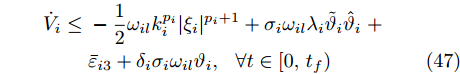
$$\begin{split} \dot{V}_i\le\; &-\frac{1}{2}\omega_{il} k_i^{p_i}|\xi_{i}|^{p_i+1}+\sigma_i\omega_{il} \lambda_i\tilde{\vartheta}_i\hat{\vartheta}_i\;+\\ &\bar{\varepsilon}_{i3}+\delta_i\sigma_i\omega_{il} \vartheta_i,\;\;\forall t\in [0,t_f) \end{split} $$ (47) 依据引理2和引理5, 以及Young不等式, 则有
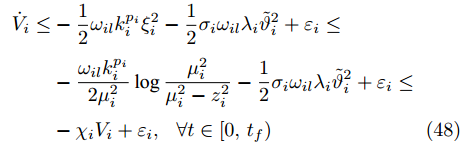
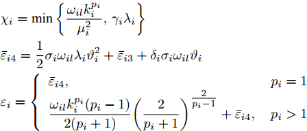
$$ \begin{split} \dot{V}_i\le&-\frac{1}{2}\omega_{il} k_i^{p_i}\xi_{i}^2-\frac{1}{2}\sigma_i\omega_{il} \lambda_i\tilde{\vartheta}_i^2+\varepsilon_i\le\\ &-\frac{\omega_{il} k_i^{p_i}}{2\mu_i^2}\log\frac{\mu_i^2}{\mu_i^2-z_i^{2}}-\frac{1}{2}\sigma_i\omega_{il} \lambda_i\tilde{\vartheta}_i^2+\varepsilon_i\le\\ &-\chi_iV_i+\varepsilon_i,\;\;\forall t\in [0,t_f) \end{split}$$ (48) 其中,
$$ \begin{split} &{\chi _i} = \min \left\{ \frac{{{\omega _{il}}k_i^{{p_i}}}}{{\mu _i^2}},{\gamma _i}{\lambda _i}\right\} \\ &{{\bar \varepsilon }_{i4}} = \frac{1}{2}{\sigma _i}{\omega _{il}}{\lambda _i}\vartheta _i^2 + {{\bar \varepsilon }_{i3}} + {\delta _i}{\sigma _i}{\omega _{il}}{\vartheta _i}\\ &{\varepsilon _i} = \left\{ \begin{array}{*{20}{l}} {{{\bar \varepsilon }_{i4}},}&{{p_i} = 1}\\ {\dfrac{{{\omega _{il}}k_i^{{p_i}}({p_i} - 1)}}{{2({p_i} + 1)}}{{\left(\dfrac{2}{{{p_i} + 1}}\right)}^{\tfrac{2}{{{p_i} - 1}}}} + {{\bar \varepsilon }_{i4}},}&{{p_i} > 1} \end{array} \right. \end{split} $$ 因此, 存在正常数
$ \chi_i^* $ 和$ \varepsilon_i^* $ 满足$$ 0<\chi_i^*\le\chi_i $$ (49) $$ 0<\varepsilon_i\le\varepsilon_i^* $$ (50) 由式(48) ~ (50), 可得
$$ \dot{V}_i\le-\chi_i^*V_i+\varepsilon_i^*,\;\forall t\in [0,t_f) $$ (51) 因此, 对
$ \forall t\in [0,t_f) $ 中, 有$$ \frac{1}{2}\log\frac{\mu_i^2}{\mu_i^2-z_i^{2}}\le V_i\le \varpi_i $$ (52) $$ \frac{\sigma_i\omega_{il} }{2\gamma_i}\tilde{\vartheta}_i^2\le V_i\le \varpi_i\;\; \qquad $$ (53) 其中,
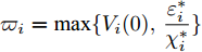
$\varpi_i = \max\{V_i(0),\dfrac{\varepsilon_i^*}{\chi_i^*}\}$ .从式(52)和式(53), 可得
$$ |z_i|\le\bar{\mu}_i = \mu_i\sqrt{1-\exp(-{2}\varpi_i)}<\mu_i $$ (54) $$ |\hat{\vartheta}_i|\le\bar{\vartheta}_i = \sqrt{\frac{2\gamma_i\varpi_i}{\sigma_i\omega_{il}}}+\vartheta_i,\;\forall t\in [0,t_f) $$ (55) 进而可推出, 对
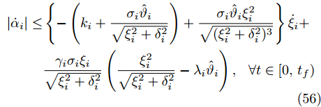
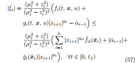
$ \forall t\in [0,t_f) $ ,$ \alpha_i $ 和$ x_{i+1} $ 有界. 接着, 对$ \alpha_i $ 和$ \xi_i $ 分别求导, 可得$$ \begin{split}|\dot{\alpha}_i|\le&\left\{-\left(k_i+\frac{\sigma_i\hat{\vartheta}_i}{\sqrt{\xi_i^2+\delta_i^2}}\right)+\frac{\sigma_i\hat{\vartheta}_i\xi_i^2}{\sqrt{(\xi_i^2+\delta_i^2)^3}}\right\}\dot{\xi}_i+\\ & \frac{\gamma_i\sigma_i\xi_i}{\sqrt{\xi_i^2+\delta_i^2}}\left(\frac{\xi_i^2}{\sqrt{\xi_i^2+\delta_i^2}} -\lambda_i\hat{\vartheta}_i\right),\;\;\forall t\in [0,t_f) \end{split}$$ (56) $$ \begin{split} |\dot{\xi}_i| =\; &\frac{(\mu_i^2+z_i^2)}{(\mu_i^2-z_i^2)^2}\Big(f_i(t,{\boldsymbol{x}},u)\;+\\ &g_i(t,{\boldsymbol{x}},u)[x_{i+1}]^{p_i}-\dot{\alpha}_{i-1}\Big)\le\\ &\frac{(\mu_i^2+z_i^2)}{(\mu_i^2-z_i^2)^2}\Big(\sum\limits_{l = 1}^{j_i}|x_{i+1}|^{q_{il}}\bar{f}_{il}(\bar{{\boldsymbol{x}}}_i)+|\dot{\alpha}_{i-1}|+\\ &\bar{g}_i(\bar{{\boldsymbol{x}}}_{i})|x_{i+1}|^{p_i}\Big),\;\;\forall t\in [0,t_f)\\[-10pt] \end{split} $$ (57) 从式(56)和式(57)可知, 对
$ \forall t\in [0,t_f) $ ,$ \dot{\xi}_i $ 和$ \dot{\alpha}_i $ 亦有界.步骤
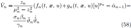
$ {\boldsymbol{n}} $ . 求$ V_n $ 的导数, 可得$$ \begin{split} \dot{V}_n =& \frac{z_n}{\mu_n^2-z_n^{2}}(f_n(t,{\boldsymbol{x}},u) + g_n(t,{\boldsymbol{x}},u)[u]^{p_n}-\dot{\alpha}_{n-1})-\\ &\frac{\sigma_n\beta_n}{\gamma_n}\tilde{\vartheta}_n\dot{\hat{\vartheta}}_n \\[-10pt]\end{split}$$ (58) 类似于式(35)的推导过程, 利用假设1和引理2, 可得
$$ |f_n(t,{\boldsymbol{x}},u)|\le \frac{1}{2}g_n(t,{\boldsymbol{x}},u)|u|^{p_n}+\psi_n(\bar{{\boldsymbol{x}}}_n) $$ (59) 其中,
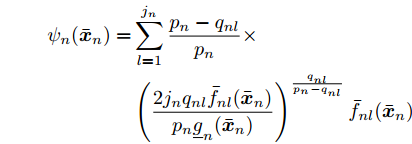
$$ \begin{split} \psi_n(\bar{{\boldsymbol{x}}}_n) = &\sum\limits_{l = 1}^{j_n}\frac{p_n-q_{nl}}{p_n}\times\\ &\left(\frac{2j_nq_{nl}\bar{f}_{nl}(\bar{{\boldsymbol{x}}}_n)}{p_n\underline{g}_n(\bar{{\boldsymbol{x}}}_n)}\right)^{\frac{q_{nl}}{p_n-q_{nl}}}\bar{f}_{nl}(\bar{{\boldsymbol{x}}}_n) \end{split}$$ 由式(59)以及命题1, 可推得
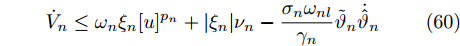
$$ \dot{V}_n\le\omega_n\xi_n[u]^{p_n}+|\xi_n|\nu_n-\frac{\sigma_n\omega_{nl} }{\gamma_n}\tilde{\vartheta}_n\dot{\hat{\vartheta}}_n $$ (60) 其中,
$\omega_n = \dfrac{\underline{g}_n(\bar{{\boldsymbol{x}}}_n)}{2}$ ,$ \nu_n = \psi_n(\bar{{\boldsymbol{x}}}_n)+|\dot{\alpha}_{n-1}| $ .由Part 1可知, 对
$ \forall t\in [0,t_f) $ ,$ |z_j|<\mu_j $ ,$j = 1, \cdots, n$ . 同时, 根据假设1和假设2,$ y_r $ 和$ \dot{y}_r $ 有界, 且$ \bar{f}_{nl} $ ,$ \underline{g}_n $ 和$ \bar{g}_n $ 连续. 此外, 由第$ n-1 $ 步设计可推得$x_1,\cdots, x_n$ ,$ \dot{\alpha}_{n-1} $ 有界,$ \forall t\in [0,t_f) $ . 因此, 运用极值定理, 对$ \forall t\in [0,t_f) $ , 有$$ 0< \omega_{nl}\le \omega_n $$ (61) $$ 0\le \nu_n\le \nu_{nm} $$ (62) 其中,
$ \omega_{nl} $ 和$ \nu_{nm} $ 为未知正常数.利用式(61)和式(62), 有
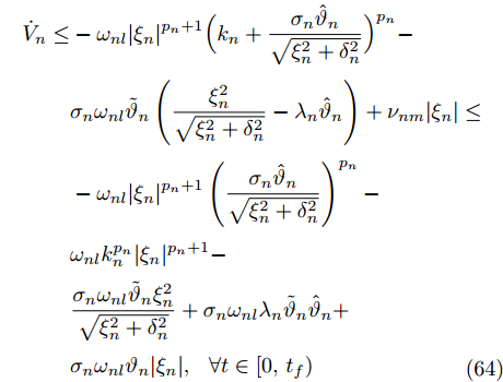
$$ \begin{split} \dot{V}_n\le\;&\omega_{nl}\xi_n[u]^{p_n}+\nu_{nm}|\xi_n|-\\& \frac{\sigma_n\omega_{nl} }{\gamma_n}\tilde{\vartheta}_n\dot{\hat{\vartheta}}_n,\;\;\forall t\in [0,t_f) \end{split} $$ (63) 根据式(16)和式(17)以及命题1和引理3, 可得
$$ \begin{split} \dot{V}_n\le&-\omega_{nl}|\xi_{n}|^{p_n+1}\Big(k_n+\frac{\sigma_n\hat{\vartheta}_n}{\sqrt{\xi_n^2+\delta_n^2}}\Big)^{p_n}-\\ &\sigma_n\omega_{nl} \tilde{\vartheta}_n\left(\frac{\xi_n^2}{\sqrt{\xi_n^2+\delta_n^2}}-\lambda_n\hat{\vartheta}_n\right)+\nu_{nm}|\xi_n|\le\\ & -\omega_{nl} |\xi_{n}|^{p_n+1}\left(\frac{\sigma_n\hat{\vartheta}_n}{\sqrt{\xi_n^2+\delta_n^2}}\right)^{p_n}-\\ &\omega_{nl} k_n^{p_n}|\xi_{n}|^{p_n+1}-\\ &\frac{\sigma_n\omega_{nl} \tilde{\vartheta}_n\xi_n^2}{\sqrt{\xi_n^2+\delta_n^2}}+\sigma_n\omega_{nl} \lambda_n\tilde{\vartheta}_n\hat{\vartheta}_n+\\ &\sigma_n\omega_{nl} \vartheta_n|\xi_n|,\;\;\forall t\in [0,t_f) \\[-10pt]\end{split}$$ (64) 其中,
$\vartheta_n = \dfrac{\nu_{nm}}{\sigma_n\omega_{nl}}$ .依据引理2和引理4, 式(64)中的项
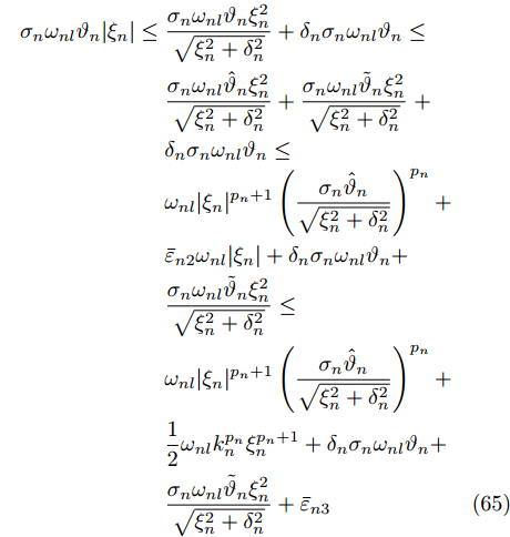
$ \sigma_n\omega_{nl}\vartheta_n|\xi_n| $ 放缩为$$ \begin{split} \sigma_n\omega_{nl} \vartheta_n|\xi_n|\le\;&\frac{\sigma_n\omega_{nl} \vartheta_n\xi_n^2}{\sqrt{\xi_n^2+\delta_n^2}}+\delta_n\sigma_n\omega_{nl} \vartheta_n\le\\ & \frac{\sigma_n\omega_{nl} \hat{\vartheta}_n\xi_n^2}{\sqrt{\xi_n^2+\delta_n^2}}+\frac{\sigma_n\omega_{nl} \tilde{\vartheta}_n\xi_n^2}{\sqrt{\xi_n^2+\delta_n^2}}\;+\\ &\delta_n\sigma_n\omega_{nl} \vartheta_n\le\\ &\omega_{nl} |\xi_n|^{p_n+1}\left(\frac{\sigma_n\hat{\vartheta}_n}{\sqrt{\xi_n^2+\delta_n^2}}\right)^{p_n}+\\ &\bar{\varepsilon}_{n2}\omega_{nl} |\xi_n|+\delta_n\sigma_n\omega_{nl}\vartheta_n+\\ &\frac{\sigma_n\omega_{nl} \tilde{\vartheta}_n\xi_n^2}{\sqrt{\xi_n^2+\delta_n^2}}\le\\ &\omega_{nl} |\xi_n|^{p_n+1}\left(\frac{\sigma_n\hat{\vartheta}_n}{\sqrt{\xi_n^2+\delta_n^2}}\right)^{p_n}+\\ &\frac{1}{2}\omega_{nl} k_n^{p_n}\xi_{n}^{p_n+1}+\delta_n\sigma_n\omega_{nl} \vartheta_n+\\ &\frac{\sigma_n\omega_{nl}\tilde{\vartheta}_n\xi_n^2}{\sqrt{\xi_n^2+\delta_n^2}}+\bar{\varepsilon}_{n3} \end{split} $$ (65) 其中,
$$ \begin{split} &{{\bar \varepsilon }_{n2}} = \left\{ {\begin{array}{*{20}{l}} {0,}&{{p_n} = 1}\\ {\dfrac{{{p_n} - 1}}{{{p_n}}}{{\left(\dfrac{1}{{{p_n}}}\right)}^{\tfrac{1}{{{p_n} - 1}}}},}&{{p_n} > 1} \end{array}} \right.\\ &{{\bar \varepsilon }_{n3}} = \left\{ {\begin{array}{*{20}{l}} {0,}&{{{\bar \varepsilon }_{n2}} = 0}\\ {\dfrac{{{{\bar \varepsilon }_{n2}}{\omega _{nl}}{p_n}}}{{{p_n} + 1}}{{\left(\dfrac{{2{{\bar \varepsilon }_{n2}}}}{{k_n^{{p_n}}({p_n} + 1)}}\right)}^{\tfrac{1}{{{p_n}}}}},}&{{{\bar \varepsilon }_{n2}} > 0} \end{array}} \right. \end{split} $$ 将式(65)代入式(64)中, 得到
$$ \begin{split} \dot{V}_n\le\;&-\frac{1}{2}\omega_{nl} k_n^{p_n}|\xi_{n}|^{p_n+1}+\sigma_n\omega_{nl} \lambda_n\tilde{\vartheta}_n\hat{\vartheta}_n\;+\\ &\bar{\varepsilon}_{n3}+\delta_n\sigma_n\omega_{nl} \vartheta_n,\;\;\forall t\in [0,t_f) \end{split} $$ (66) 根据引理2和引理5, 以及Young不等式, 可得
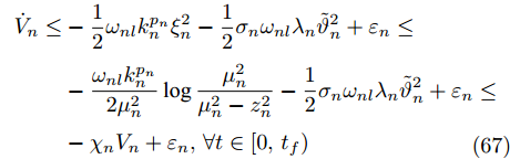
$$ \begin{split} \dot{V}_n\le&-\frac{1}{2}\omega_{nl} k_n^{p_n}\xi_{n}^2-\frac{1}{2}\sigma_n\omega_{nl} \lambda_n\tilde{\vartheta}_n^2+\varepsilon_n\le\\ &-\frac{\omega_{nl} k_n^{p_n}}{2\mu_n^2}\log\frac{\mu_n^2}{\mu_n^2-z_n^{2}}-\frac{1}{2}\sigma_n\omega_{nl} \lambda_n\tilde{\vartheta}_n^2+\varepsilon_n\le\\ &-\chi_nV_n+\varepsilon_n,\forall t\in [0,t_f) \\[-10pt]\end{split} $$ (67) 其中,
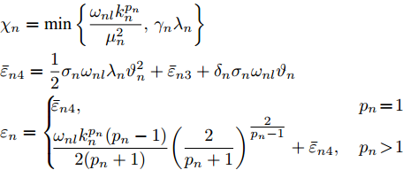
$$ \begin{split} &{\chi _n} = \min \left\{ \frac{{{\omega _{nl}}k_n^{{p_n}}}}{{\mu _n^2}},{\gamma _n}{\lambda _n}\right\} \\ &{{\bar \varepsilon }_{n4}} = \frac{1}{2}{\sigma _n}{\omega _{nl}}{\lambda _n}\vartheta _n^2 + {{\bar \varepsilon }_{n3}} + {\delta _n}{\sigma _n}{\omega _{nl}}{\vartheta _n}\\ &{\varepsilon _n} = \left\{ {\begin{array}{*{20}{l}} {{{\bar \varepsilon }_{n4}},}&{{p_n} = 1}\\ {\dfrac{{{\omega _{nl}}k_n^{{p_n}}({p_n} - 1)}}{{2({p_n} + 1)}}{{\left(\dfrac{2}{{{p_n} + 1}}\right)}^{\tfrac{2}{{{p_n} - 1}}}} + {{\bar \varepsilon }_{n4}},}&{{p_n} > 1} \end{array}} \right. \end{split} $$ 因此, 存在正常数
$ \chi_n^* $ 和$ \varepsilon_n^* $ , 使得$$ 0<\chi_n^*\le \chi_n $$ (68) $$ 0<\varepsilon_n\le\varepsilon_n^* \; $$ (69) 根据式(67) ~ (69), 可得
$$ \dot{V}_n\le-\chi_n^*V_n+\varepsilon_n^*,\;\;\forall t\in [0,t_f) $$ (70) 因此, 对
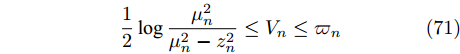
$ \forall t\in [0,t_f) $ , 有$$ \frac{1}{2}\log\frac{\mu_n^2}{\mu_n^2-z_n^{2}}\le V_n\le \varpi_n $$ (71) $$ \frac{\sigma_n\omega_{nl} }{2\gamma_n}\tilde{\vartheta}_n^2\le V_n\le \varpi_n\;\;\;\;\;\;\; $$ (72) 其中,
$\varpi_n = \max\{V_n(0),\dfrac{\varepsilon_n^*}{\chi_n^*}\}$ .由式(71)和式(72), 可得
$$ |z_n|\le \bar{\mu}_n = \mu_n\sqrt{1-\exp(-{2}\varpi_n)}<\mu_n\;\;\;\;\; $$ (73) $$ |\hat{\vartheta}_n|\le\sqrt{\bar{\vartheta}_n = \frac{2\gamma_n\varpi_n}{\sigma_n\omega_{nl}}}+\vartheta_n,\;\; \forall t\in [0,t_f) $$ (74) 故可推出, 对
$ \forall t\in [0,t_f) $ ,$ u $ 有界.由步骤 1 ~
$n $ 可知, 存在紧子集$\Xi' = [-\bar{\mu}_1,\bar{\mu}_1]\,\times \cdots\times [-\bar{\mu}_n, \bar{\mu}_n]\times [-\bar{\vartheta}_1,\bar{\vartheta}_1]\times\cdots\times[-\bar{\vartheta}_n,\bar{\vartheta}_n]\subset \Xi$ , 使得闭环系统在$ [0,t_f) $ 上存在唯一解$ {\boldsymbol{\eta}}(t)\in \Xi' $ . 根据引理1, 可得:$ t_f = +\infty $ , 即, 对$ \forall t \in [0,+\infty) $ ,$|z_i| < \mu_i$ ,$i = 1, \cdots,n$ .Part 3. 重复Part 2中的步骤1 ~ n, 可得
$x_1,\cdots, x_n$ ,$\alpha_1,\cdots,\alpha_{n-1}$ 和$ u $ 均有界,$ \forall t \in [0,+\infty) $ . 另外, 从式(54)可知, 通过减小$ \mu_1 $ 和$ \varpi_1 $ 可将输出跟踪误差$ z_1 $ 收敛到任意小的残差集. □注 4. 不同于文献[20-25]中提出的控制方案, 本文采用积分反推技术和障碍李雅普诺夫方法解决了高阶非线性系统中幂次未知和系统函数不确定的问题, 且所设计控制策略不依赖于未知幂次的上界信息.
3. 仿真算例
为了验证本文所提控制算法的有效性与通用性, 考虑如下两个高阶非线性系统
$$ {\Sigma _1}:\left\{ \begin{aligned} &{{{\dot x}_1} = {f_{1,{\Sigma _1}}} + {g_{1,{\Sigma _1}}}{{[{x_2}]}^{{p_1}}}}\\ &{{{\dot x}_2} = {f_{2,{\Sigma _1}}} + {g_{2,{\Sigma _1}}}{{[u]}^{{p_2}}}}\\ &{y = {x_1}} \end{aligned} \right. $$ (75) $$ {\Sigma _2}:\left\{ \begin{aligned} &{{{\dot x}_1} = {f_{1,{\Sigma _2}}} + {g_{1,{\Sigma _2}}}{{[{x_2}]}^{{p_1}}}}\\ &{{{\dot x}_2} = {f_{2,{\Sigma _2}}} + {g_{2,{\Sigma _2}}}{{[u]}^{{p_2}}}}\\ &{y = {x_1}} \end{aligned} \right. $$ (76) 其中,
$p_1 = {5}/{3}$ ,$p_2 ={7}/{3}$ ,$ f_{1,\Sigma_1} = x_1\cos (t) $ ,$g_{1,\Sigma_1} = 3+ 0.5\sin (t)$ ,$f_{2,\Sigma_1} = x_1+2\sin (x_1x_2)$ ,$g_{2,\Sigma_1} = 2+ 0.1\sin (t)$ ,$f_{1,\Sigma_2} \;= \;(0.5x_1\; +\; 1)\cos (t)$ ,$g_{1,\Sigma_2} = 2 + 0.1\sin (t)$ ,$f_{2,\Sigma_2} = \cos (x_1 )\exp(2x_2\sin (x_1 )) + x_1x_2\sin (t)$ ,$g_{2,\Sigma_2} = 1$ , 期望参考信号$y_r(t) = \dfrac{\pi}{2}(1 - \exp( -0.1t^2)) \sin (t)$ .在仿真中, 系统
$ \Sigma_i $ 和自适应参数$ \hat{\vartheta}_i $ 的初始值设置为$ [x_1(0),x_2(0)]^{\rm{T}} = [-0.5,0.4]^{\rm{T}} $ ,$ \hat{\vartheta}_i(0) = 0 $ ,$i = 1,2$ . 控制器参数$ k_1 = 2 $ ,$ k_2 = 1 $ ,$ \mu_1 = 4 $ ,$ \mu_2 = 2 $ ,$ \sigma_1 = 3 $ ,$ \sigma_2 = 2 $ ,$ \gamma_1 = 2 $ ,$ \gamma_2 = 3 $ ,$ \delta_1 = \delta_2 = 0.01 $ 和$ \lambda_1 = \lambda_2 = 0.002 $ , 其中,$ \mu_1 = 4>|z_1(0)| = 0.5 $ ,$\mu_2 = 2 > |z_2(0)| = {106}/{315}$ . 系统$ \Sigma_1 $ 和$ \Sigma_2 $ 的仿真结果如图2 ~ 4所示. 图2刻画了输出跟踪误差$ y-y_r $ 的变化情况, 图3给出系统的控制信号$ u $ , 图4描述了自适应参数$ \hat{\vartheta}_1 $ 和$ \hat{\vartheta}_2 $ . 从仿真结果可以看出, 本文所提自适应控制策略既能使系统$ \Sigma_1 $ 和$ \Sigma_2 $ 的输出跟踪误差收敛到原点附近的较小邻域内, 又能确保闭环系统的所有信号有界.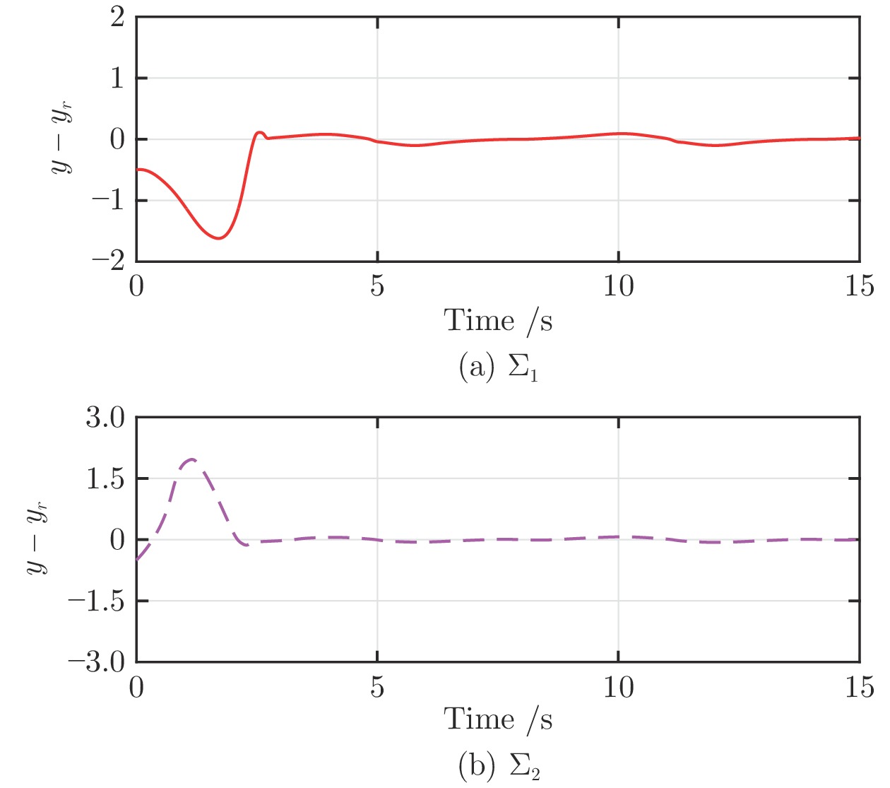 图 2 系统
$\Sigma_1$ 和$\Sigma_2$ 的输出跟踪误差$y-y_r$ Fig. 2 Output tracking errors$y-y_r$ of systems$\Sigma_1$ and$\Sigma_2$ 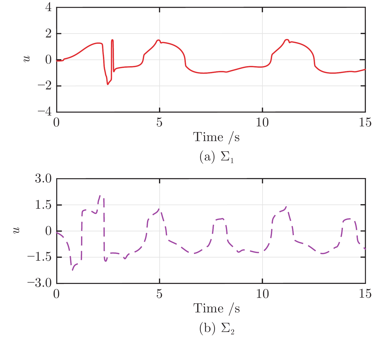 图 3 系统
$\Sigma_1$ 和$\Sigma_2$ 的控制信号$u$ Fig. 3 Control signals$u$ of systems$\Sigma_1$ and$\Sigma_2$  图 4 系统
$\Sigma_1$ 和$\Sigma_2$ 的自适应参数$\hat{\vartheta}_1$ 和$\ \hat{\vartheta}_2$ Fig. 4 Adaptive parameters$\hat{\vartheta}_1$ and$\hat{\vartheta}_2$ of systems$\Sigma_1$ and$\Sigma_2$ 为进一步验证本文控制算法的幂次无关特性, 在系统初始值与控制器参数不变的条件下, 对具有不同幂次
$ p_1 $ 和$ p_2 $ 的系统$ \Sigma_1 $ 进行仿真测试. 仿真结果如图5和图6所示. 图5为系统$ \Sigma_1 $ 在不同幂次$ p_1 $ 和$ p_2 $ 条件下的输出跟踪误差$ y-y_r $ , 图6为相应的控制信号$ u $ . 仿真结果表明, 在不同幂次条件下, 该控制器仍然可以保证闭环系统获得良好的控制性能. 图 5 系统
$\Sigma_1$ 在不同幂次下的跟踪误差$y-y_r$ Fig. 5 Output tracking errors$y-y_r$ of system$\Sigma_1$ under various powers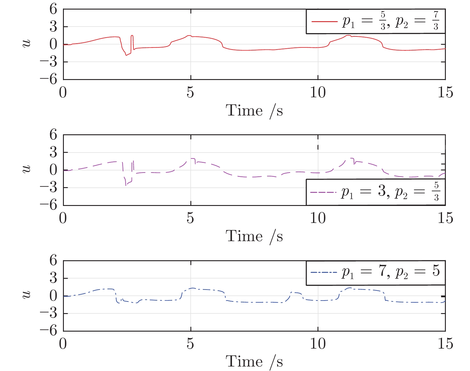 图 6 系统
$\Sigma_1$ 在不同幂次下的控制信号$u$ Fig. 6 Control signals$u$ of system$\Sigma_1$ under various powers4. 结束语
针对一类具有未知幂次的高阶不确定非线性系统, 提出了一种基于障碍李雅普诺夫函数的自适应控制算法. 在无需知晓系统函数先验知识的条件下, 所提控制算法有效克服了系统幂次未知与模型不确定带来的技术挑战. 该算法的显著特点是所设计的自适应控制器均与系统幂次无关. 最后, 仿真结果验证了本文控制算法的有效性与通用性.
今后的研究方向包括将本文所提方法推广到具有未知幂次的高阶非线性系统的输出反馈控制设计[34]. 此外, 为验证本文方法的实用性, 将本文所提控制策略应用于实际系统[35]亦是我们未来研究的目标.
-
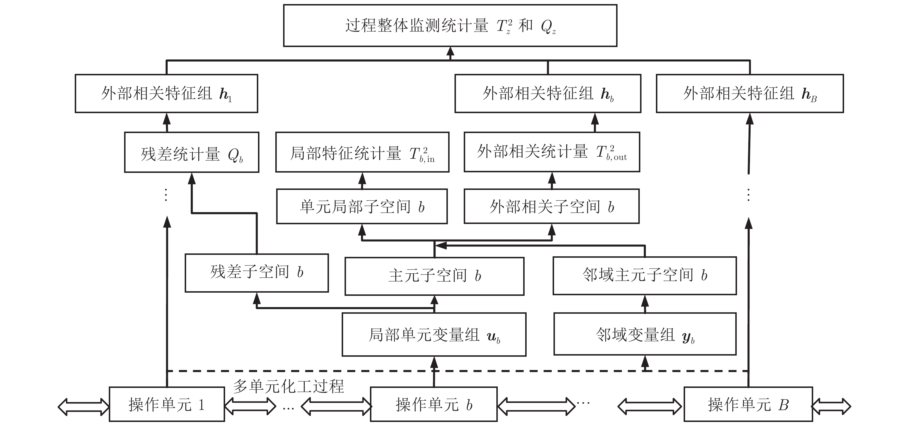
图 1 基于局部−整体相关特征的分层监测设计框架
Fig. 1 Framework of the local-global correlation feature-based hierarchical monitoring
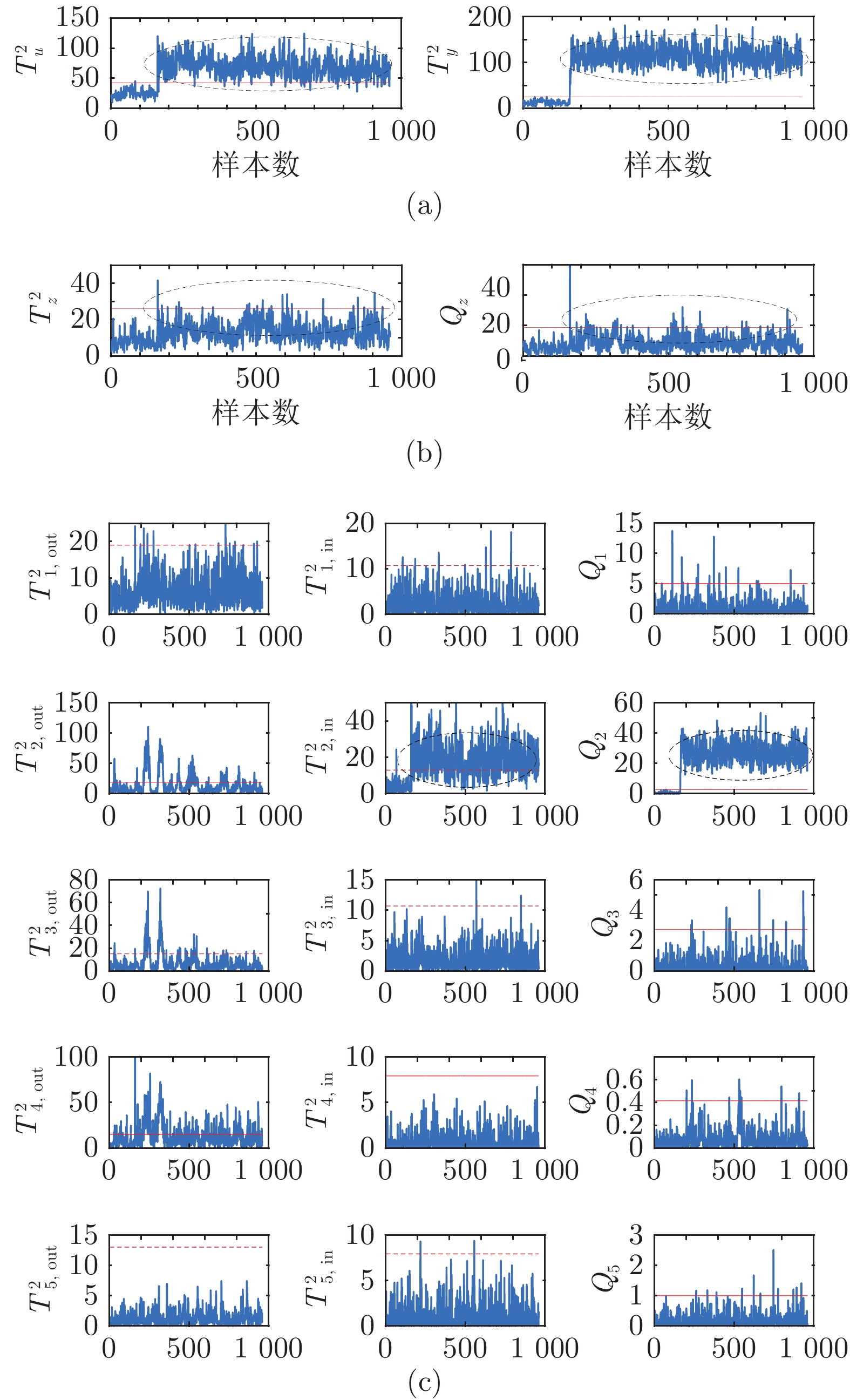
图 3 TE过程故障4的监测效果 ((a)经典CCA监测结果; (b)分层监测整体监测结果; (c)分层监测局部监测效果)
Fig. 3 Monitoring results for the TE fault 4 ((a) Conventional CCA method; (b) Global monitoring using hierarchical method; (c) Local monitoring using hierarchical method)
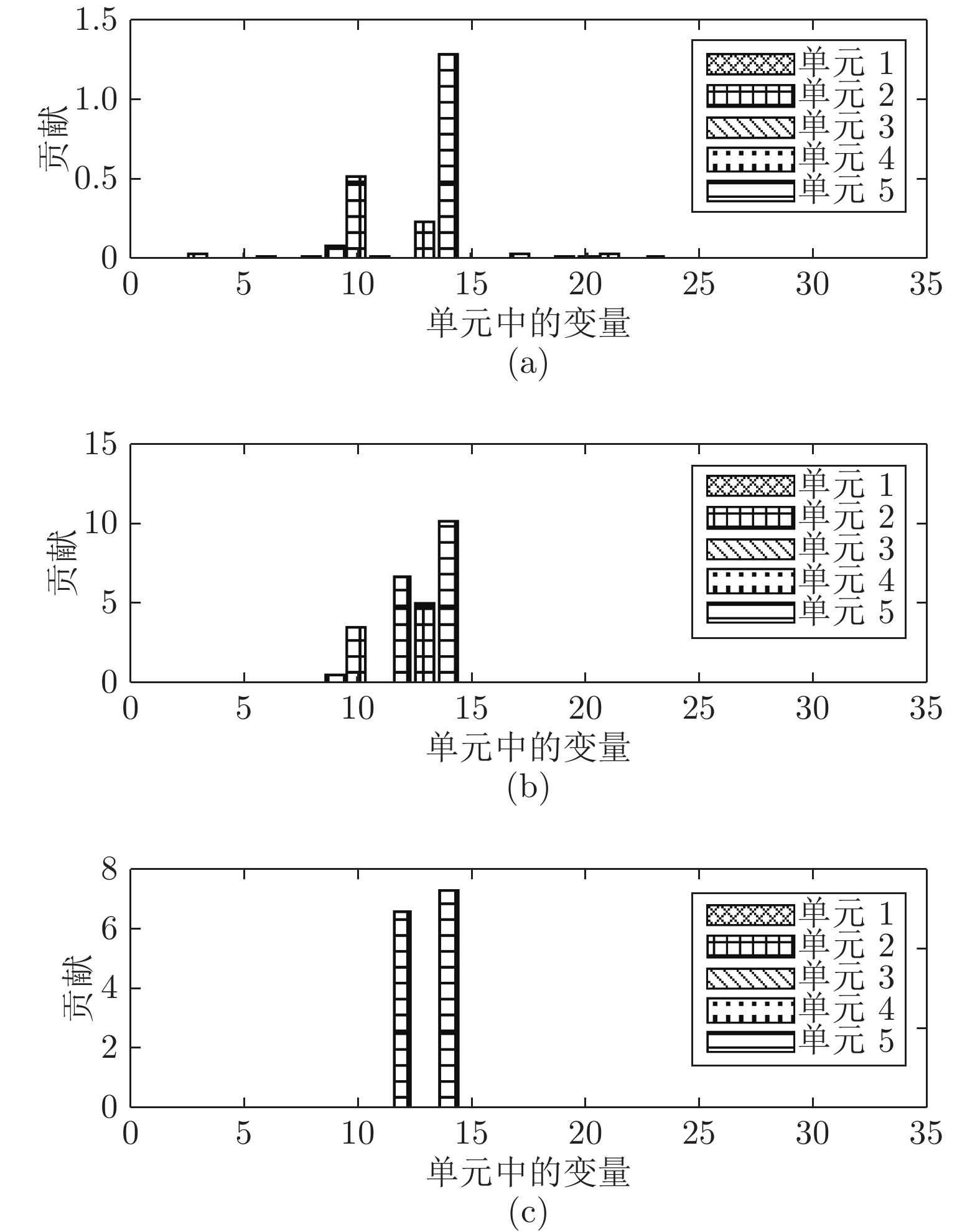
图 4 TE过程故障4的分层贡献图((a)
$T_{b,{\rm out}}^2$ ; (b)$T_{b,{\rm in}}^2$ ; (c)${Q_b}$ )Fig. 4 Contribution plots for the TE fault 4 ((a)
$T_{b,{\rm out}}^2$ ; (b)$T_{b,{\rm in}}^2$ ; (c)${Q_b}$ )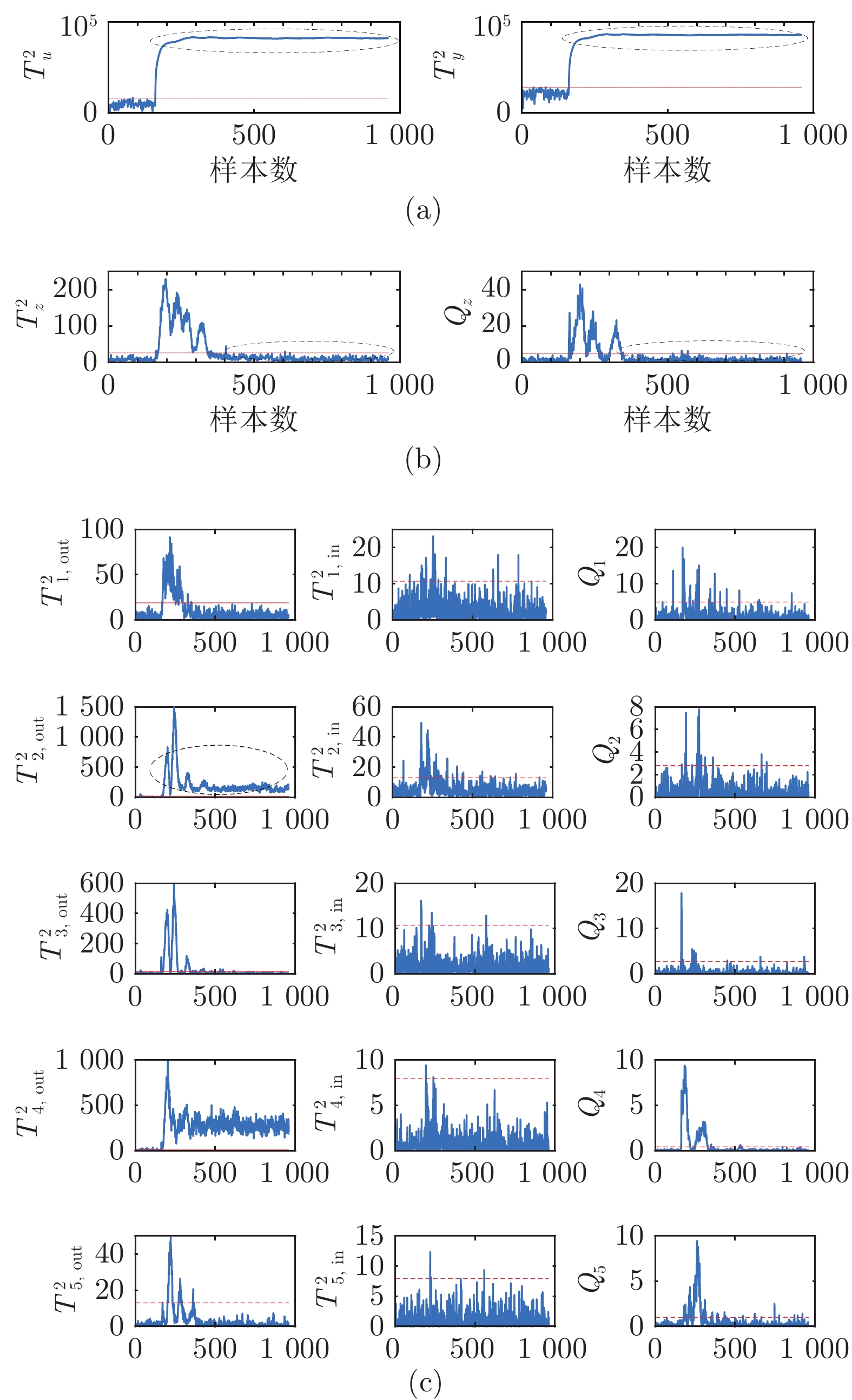
图 5 TE过程故障5的监测效果 ((a)经典CCA监测结果; (b)分层监测整体监测结果; (c)分层监测局部监测效果)
Fig. 5 Fault detection results for the TE fault 5 ((a) Conventional CCA method; (b) Global monitoring using hierarchical method; (c) Local monitoring using hierarchical method)

图 6 TE过程故障5的分层监测贡献图 ((a)
$T_z^2$ 和${Q_z}$ ; (b)$T_{b,{\rm out}}^2$ ; (c)$T_{b,{\rm in}}^2$ ; (d)${Q_b}$ ; (e)控制补偿后$T_{b,{\rm out}}^2$ )Fig. 6 Contribution plots for the TE fault 5 ((a)
$T_z^2$ and${Q_z}$ ; (b)$T_{b,{\rm out}}^2$ ; (c)$T_{b,{\rm in}}^2$ ; (d)${Q_b}$ ; (e)$T_{b,{\rm out}}^2$ after compensation)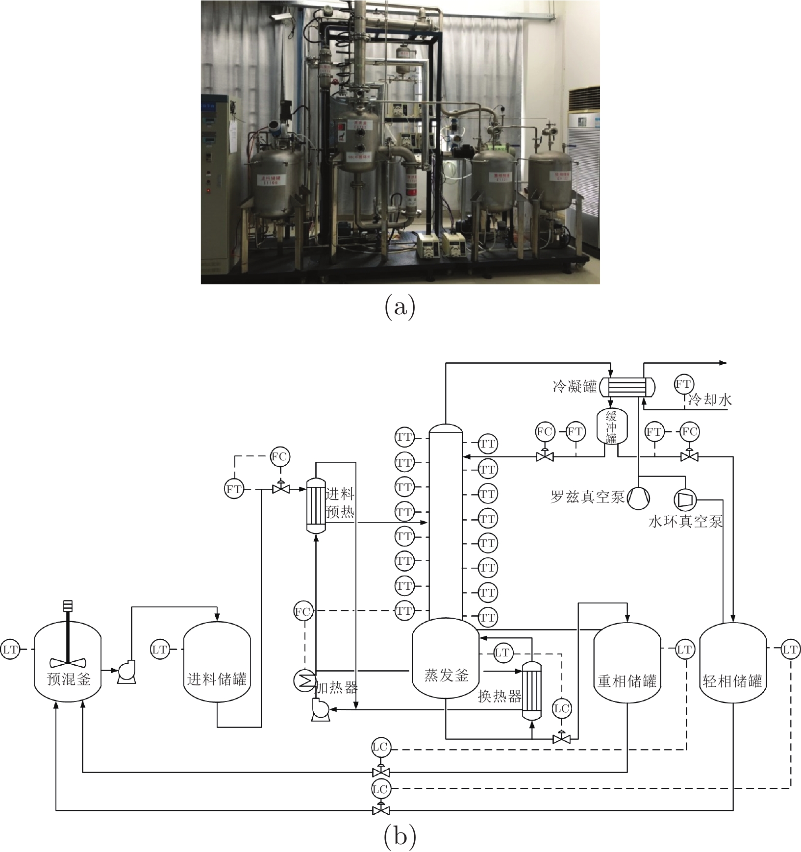
图 7 实验室甘油精馏装置与流程图((a)设备图; (b)流程图)
Fig. 7 Lab-scale glycerin distillation process ((a) Equipment diagram; (b) Simplified flowchart)
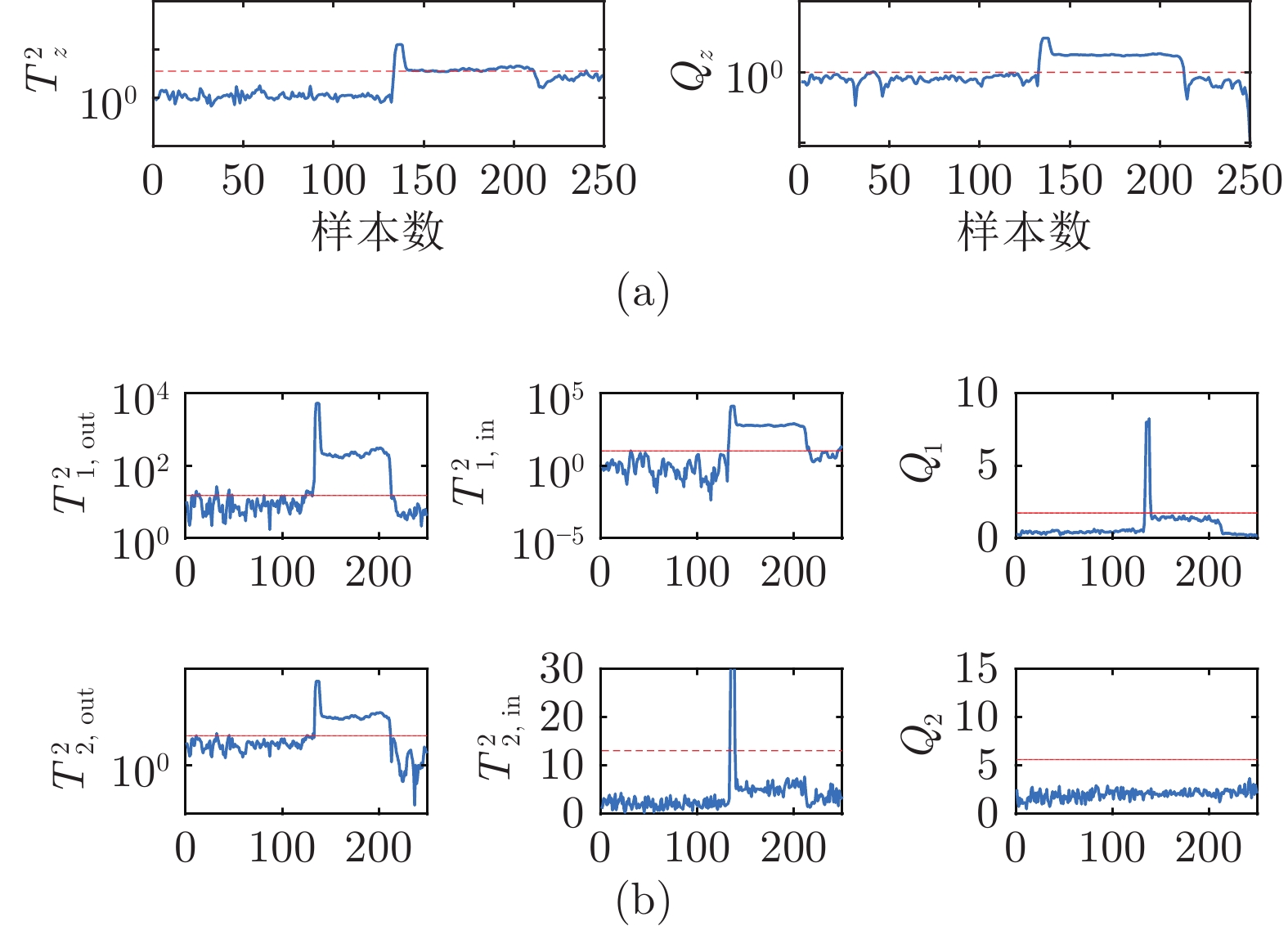
图 8 精馏过程故障1的分层故障检测效果 ((a)整体监测统计量; (b)局部监测统计量)
Fig. 8 Fault detection results for the distillation process fault 1 ((a) Global monitoring statistics; (b) Local monitoring statistics)
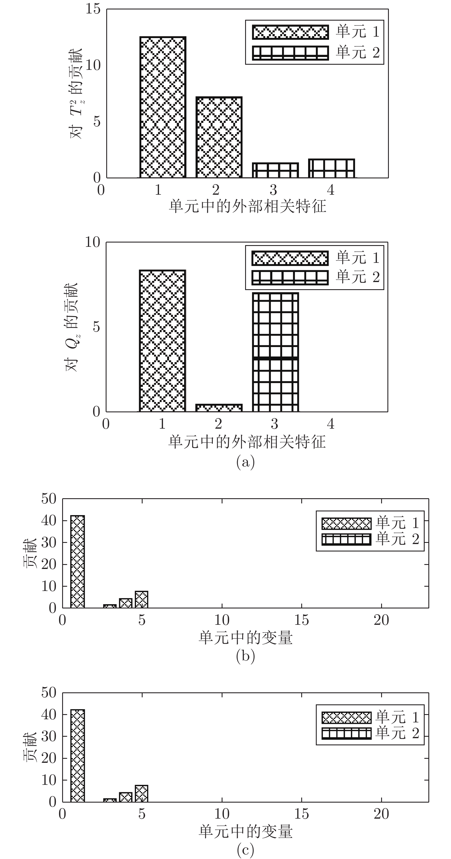
图 9 精馏过程故障1分层监测贡献图((a)
$T_z^2$ 和${Q_z}$ ; (b)$T_{b,{\rm out}}^2$ ; (c)$T_{b,{\rm in}}^2$ )Fig. 9 Contribution plots for the distillation fault 1 ((a)
$T_z^2$ and${Q_z}$ ; (b)$T_{b,{\rm out}}^2$ ; (c)$T_{b,{\rm in}}^2$ )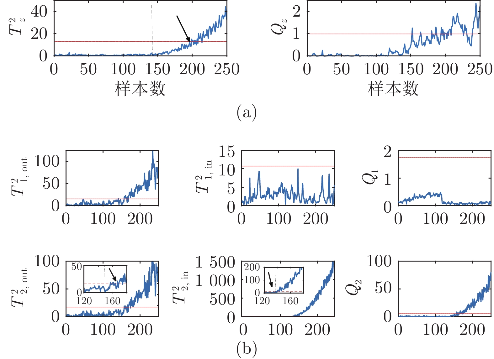
图 10 精馏过程故障2的分层故障检测效果((a)整体监测统计量; (b)局部监测统计量)
Fig. 10 Fault detection results for the distillation process fault 2 ((a) Global monitoring statistics; (b) Local monitoring statistics)
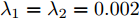
表 1 TE过程的典型操作单元和对应变量
Table 1 Operation units and corresponding variables in the TE process
单元 变量描述 变量名称 符号 进料 A 进料 (流1) XMEAS(1) $\boxed1$ D 进料 (流2) XMEAS(2) $\boxed2$ E 进料 (流3) XMEAS(3) $\boxed3$ A 和 C 进料 XMEAS(4) $\boxed4$ D 进料 XMV(1) A 进料流量 XMV(3) E 进料流量 XMV(2) A 和 C 进料流量 XMV(4) 反应器 反应器进料量 XMEAS(6) $\boxed6$ 反应器压力 XMEAS(7) $\boxed7$ 反应器液位 XMEAS(8) $\boxed8$ 反应器温度 XMEAS(9) $\boxed9$ 反应器水温 XMEAS(21) $\boxed{21}$ 反应器冷却水流量 XMV(10) 冷凝器冷却水流量 XMV(11) 分离器 分离器温度 XMEAS(11) $\boxed{11}$ 分离器液位 XMEAS(12) $\boxed{12}$ 分离器压力 XMEAS(13) $\boxed{13}$ 分离器底物流量 XMEAS(14) $\boxed{14}$ 分离器水温度 XMEAS(22) $\boxed{22}$ 分离器液流量 XMV(7) 汽提塔 汽提塔液位 XMEAS(15) $\boxed{15}$ 汽提塔压力 XMEAS(16) $\boxed{16}$ 汽提塔底物流量 XMEAS(17) $\boxed{17}$ 汽提塔温度 XMEAS(18) $\boxed{18}$ 汽提塔蒸汽流量 XMEAS(19) $\boxed{19}$ 汽提塔产物流量 XMV(8) 汽提塔蒸汽阀开度 XMV(9) 压缩 再循环流量 XMEAS(5) $\boxed5$ 排放速度 XMEAS(10) $\boxed{10}$ 压缩机功率 XMEAS(20) $\boxed{20}$ 压缩机再循环阀 XMV(5) 排放阀 XMV(6)  下载: 导出CSV
表 2 分层监测对于21个故障测试集的监测效果
Table 2 Hierarchical monitoring results for the 21 faults in TE process
编码 单元及过程 进料单元 反应器单元 分离器单元 汽提塔单元 压缩单元 过程整体 故障描述/统计量 $T_{1,{\rm out}}^2$ $T_{1,{\rm in}}^2$ ${Q_1}$ $T_{2,{\rm out}}^2$ $T_{2,{\rm in}}^2$ ${Q_2}$ $T_{3,{\rm out}}^2$ $T_{3,{\rm in}}^2$ ${Q_3}$ $T_{4,{\rm out}}^2$ $T_{4,{\rm in}}^2$ ${Q_4}$ $T_{5,{\rm out}}^2$ $T_{5,{\rm in}}^2$ ${Q_5}$ $T_z^2$ ${Q_z}$ 1 A/C 进料比率, B 成分不变 (阶跃) 0.99 0.31 0.04 0.77 0.26 0.06 0.44 0.04 0.07 1 0.06 0.98 0.17 0.02 0.23 1 1 2 B 成分, A/C 进料比率不变 (阶跃) 0.92 0.02 0.27 0.95 0.22 0.03 0.92 0.14 0.06 0.99 0.06 0.89 0.99 0.01 0.42 0.98 0.98 3 D 的进料温度 (阶跃) 0.01 0.01 0.01 0.32 0.02 0.00 0.14 0.01 0.00 0.20 0 0.01 0 0.01 0.09 0.01 0.02 4 反应器冷却水入口温度 (阶跃) 0.02 0.01 0.02 0.25 0.75 1 0.12 0.00 0.01 0.21 0 0.01 0 0.00 0.01 0.03 0.06 5 冷凝器冷却水入口温度 (阶跃) 0.16 0.03 0.04 0.99 0.09 0.03 0.23 0.01 0.02 1 0.00 0.19 0.07 0.00 0.13 0.22 0.18 6 A 进料损失 (阶跃) 0.99 0.91 1 1 0.98 0.96 0.98 0.82 0.98 0.99 0.96 0.97 0.99 0.92 0.99 0.99 0.99 7 C 存在压力损失 (阶跃) 0.98 1 0.87 0.98 0.22 0.09 0.38 0.03 0.04 0.76 0.01 0.22 0.24 0.01 0.27 1 0.98 8 A、B、C 进料成分 (随机) 0.78 0.10 0.16 0.97 0.48 0.13 0.90 0.03 0.35 0.94 0.11 0.68 0.87 0.02 0.61 0.97 0.89 9 D 的进料温度 (随机) 0.00 0.01 0.01 0.27 0.02 0.01 0.14 0.01 0.01 0.16 0 0.01 0 0.00 0.02 0.01 0.02 10 C 的进料温度 (随机) 0.08 0.02 0.02 0.43 0.04 0.02 0.33 0.01 0.00 0.46 0.00 0.81 0.07 0.00 0.10 0.29 0.13 11 反应器冷却水入口温度 (随机) 0.11 0.01 0.01 0.39 0.61 0.70 0.17 0.01 0.01 0.42 0.00 0.05 0 0.01 0.02 0.20 0.27 12 冷凝器冷却水入口温度 (随机) 0.74 0.22 0.25 0.95 0.60 0.29 0.94 0.28 0.65 0.96 0.06 0.89 0.34 0.03 0.83 0.96 0.91 13 反应动态 (慢偏移) 0.77 0.19 0.30 0.92 0.72 0.39 0.89 0.10 0.48 0.95 0.24 0.86 0.85 0.03 0.89 0.94 0.95 14 反应器冷却水阀门 (粘滞) 0.75 0.01 0.00 1 0.97 0.12 0.36 0.07 0.01 0.88 0.01 0.01 0.04 0.01 0.01 1 1 15 冷凝器冷却水阀门 (粘滞) 0.01 0.01 0.01 0.29 0.02 0.01 0.18 0.00 0.01 0.23 0 0.03 0.00 0.00 0.03 0.02 0.06 16 未知 0.03 0.02 0.01 0.37 0.03 0.01 0.26 0.00 0.00 0.40 0 0.85 0.03 0.01 0.05 0.15 0.11 17 未知 0.64 0.02 0.01 0.95 0.94 0.44 0.35 0.04 0.02 0.76 0.00 0.22 0.03 0.01 0.03 0.84 0.85 18 未知 0.88 0.82 0.83 0.92 0.87 0.79 0.91 0.12 0.87 0.90 0.75 0.88 0.80 0.71 0.85 0.88 0.88 19 未知 0.01 0.02 0.01 0.24 0.08 0.01 0.14 0.01 0.01 0.16 0 0.12 0.01 0.32 0.66 0.01 0.03 20 未知 0.03 0.02 0.01 0.61 0.02 0.01 0.38 0.05 0.39 0.81 0.00 0.23 0.47 0.01 0.89 0.32 0.43 21 流 4 的阀门固定在稳态位置 0.01 0.00 0.00 0.66 0.44 0.01 0.87 0.00 0.01 0.73 0.00 0.45 0.31 0.00 0.02 0.41 0.84
下载: 导出CSV
表 3 甘油精馏过程中的监测变量
Table 3 Measured variables in the distillation process
单元 1 变量名称 单元 2 变量名称 1 进料流量 1 进料储罐液位 2 灵敏板温度 2~13 塔板温度1~12 3 塔底液位 14 冷却水流量 4 塔顶回流 15 重相储灌液位 5 塔顶产品流 16 轻相储罐液位
下载: 导出CSV
-
[1] 柴天佑, 丁进良. 流程工业智能优化制造. 中国工程科学, 2018, 20(4): 51−58Chai Tian-You, Ding Jin-Liang. Smart and optimal manufacturing for process industry. Strategic Study of CAE, 2018, 20(4): 51−58 [2] 刘强, 卓洁, 郎自强, 秦泗钊. 数据驱动的工业过程运行监控与自优化研究展望. 自动化学报, 2018, 44(11): 1944−1956Liu Qiang, Zhuo Jie, Lang Zi-Qiang, Qin S Joe. Perspectives on data-driven operation monitoring and self-optimization of industrial processes. Acta Automatica Sinica, 2018, 44(11): 1944−1956 [3] 钱锋, 杜文莉, 钟伟民, 唐漾. 石油和化工行业智能优化制造若干问题及挑战. 自动化学报, 2017, 43(6): 893−901Qian Feng, Du Wen-Li, Zhong Wei-Min, Tang Yang. Problems and challenges of smart optimization manufacturing in petrochemical industries. Acta Automatica Sinica, 2017, 43(6): 893−901 [4] Qin S J. Process data analytics in the era of big data. AIChE Journal, 2014, 60(9): 3092−3100 doi: 10.1002/aic.14523 [5] 赵春晖, 余万科, 高福荣. 非平稳间歇过程数据解析与状态监控—回顾与展望, 自动化学报, 2020, DOI: 10.16383/j.aas.c190586Zhao Chun-Hui, Yu Wan-Ke, Gao Fu-Rong. Data analytics and condition monitoring methods for nonstationary batch processes—current status and future, Acta Automatica Sinica, 2020, DOI: 10.16383/j.aas.c190586 [6] Wang Y Q, Si Y B, Huang B, and Lou Z J. Survey on the theoretical research and engineering applications of multivariate statistics process monitoring algorithms: 2008–2017. The Canadian Journal of Chemical Engineering, 2018, 96(10): 2073−2085 doi: 10.1002/cjce.23249 [7] Ge Z Q. Review on data-driven modeling and monitoring for plant-wide industrial processes. Chemometrics and Intelligent Laboratory Systems, 2017, 171: 16−25 [8] Jiang Q C, Yan X F, Huang B. Review and perspectives of data-driven distributed monitoring for industrial plant-wide processes. Industrial and Engineering Chemistry Research, 2019, 58(29): 12899−12912 [9] 郭小萍, 刘诗洋, 李元. 基于稀疏残差距离的多工况过程故障检测方法研究. 自动化学报, 2019, 45(3): 617−625Guo Xiao-Ping, Liu Shi-Yang, Li Yuan. Fault detection of multi-mode processes employing sparse residual distance. Acta Automatica Sinica, 2019, 45(3): 617−625 [10] Ding S X, Data-driven Design of Fault Diagnosis and Fault-tolerant Control Systems: Springer London, 2014. [11] Zhang Y W, Zhou H, Qin S J. Decentralized fault diagnosis of large-scale processes using multiblock kernel principal component analysis. Acta Automatica Sinica, 2010, 36(4): 593−597 [12] Zhao C H, Sun H. Dynamic distributed monitoring strategy for large-scale nonstationary processes subject to frequently varying conditions under closed-loop control. IEEE Transactions on Industrial Electronics, 2019, 66(6): 4749−4758 doi: 10.1109/TIE.2018.2864703 [13] Shang C, Ji H Q, Huang X L, Yang F, Huang D X. Generalized grouped contributions for hierarchical fault diagnosis with group Lasso. Control Engineering Practice, 2019, 93: 104193 doi: 10.1016/j.conengprac.2019.104193 [14] 邹筱瑜, 王福利, 常玉清, 王敏, 蔡庆宏. 基于分层分块结构的流程工业过程运行状态评价及非优原因追溯. 自动化学报, 2019, 45(2): 315−324Zou Xiao-Yu, Wang Fu-Li, Chang Yu-Qing, Wang Min, Cai Qing-Hong. Plant-wide process operating performance assessment and non-optimal cause identication based on hierarchical multi-block structure. Acta Automatica Sinica, 2019, 45(2): 315−324 [15] Jiang Q C, Huang B. Distributed monitoring for large-scale processes based on multivariate statistical analysis and Bayesian method. Journal of Process Control, 2016, 46: 75−83 doi: 10.1016/j.jprocont.2016.08.006 [16] 罗娜, 蒋勇, 叶贞成, 杜文莉, 钱锋. 基于集成建模方法的乙二醇全流程模拟. 化工学报, 2009, 60(1): 151−156 doi: 10.3321/j.issn:0438-1157.2009.01.022Luo Na, Jiang Yong, Ye Zhen-Cheng, Du Wen-Li, Qian Feng. Simulation of ethylene glycol process based on integrated modeling method. Chinese Journal of Chemical Engineering, 2009, 60(1): 151−156 doi: 10.3321/j.issn:0438-1157.2009.01.022 [17] 文成林, 吕菲亚, 包哲静, 刘妹琴. 基于数据驱动的微小故障诊断方法综述. 自动化学报, 2016, 42(9): 1285−1299Wen Cheng-Lin, Lv Fei-Ya, Bao Zhe-Jing, Liu Mei-Qin. A review of data driven-based incipient fault diagnosis. Acta Automatica Sinica, 2016, 42(9): 1285−1299 [18] 杨浩, 姜斌, 周东华. 互联系统容错控制的研究回顾与展望. 自动化学报, 2017, 43(1): 9−19Yang Hao, Jiang Bin, Zhou Dong-Hua. Review and perspectives on fault tolerant control for interconnected systems. Acta Automatica Sinica, 2017, 43(1): 9−19 [19] Chen Z W, Ding S X, Zhang K, Li Z B, Hu Z K. Canonical correlation analysis-based fault detection methods with application to alumina evaporation process. Control Engineering Practice, 2016, 46: 51−58 doi: 10.1016/j.conengprac.2015.10.006 [20] 曹玉苹, 黄琳哲, 田学民. 一种基于 DIOCVA 的过程监控方法. 自动化学报, 2015, 41(12): 2072−2080Cao Yu-Ping, Huang Lin-Zhe, Tian Xue-Min. A process monitoring method using dynamic input-output canonical variate analysis. Acta Automatica Sinica, 2015, 41(12): 2072−2080 [21] Shi L K, Tong C D, Lan T, Shi X H. Statistical process monitoring based on ensemble structure analysis, IEEE/CAA Journal of Automatica Sinica, 2018, DOI: 10.1109/JAS. 2017.7510877 [22] 彭开香, 马亮, 张凯. 复杂工业过程质量相关的故障检测与诊断技术综述. 自动化学报, 2017, 43(3): 349−365Peng Kai-Xiang, Ma Liang, Zhang Kai. Review of quality-related fault detection and diagnosis techniques for complex industrial processes. Acta Automatica Sinica, 2017, 43(3): 349−365 [23] Ge Z Q, Song Z H. Distributed PCA model for plant-wide process monitoring. Industrial and Engineering Chemistry Research, 2013, 52(5): 1947−1957 [24] Liu Q, Qin S J, Chai T Y. Multiblock concurrent PLS for decentralized monitoring of continuous annealing processes. IEEE Transactions on Industrial Electronics, 2014, 61(61): 6429−6437 [25] Qin S J, Valle S, Piovoso M J. On unifying multiblock analysis with application to decentralized process monitoring. Journal of Chemometrics, 2001, 15(9): 715−742 doi: 10.1002/cem.667 [26] Ge Z Q. Quality prediction and analysis for large-scale processes based on multi-level principal component modeling strategy. Control Engineering Practice, 2014, 31(1): 9−23 [27] Jiang Q C, Ding S X, Wang Y, Yan X F. Data-driven distributed local fault detection for large-scale processes based on the GA-regularized canonical correlation analysis. IEEE Transactions on Industrial Electronics, 2017, 64(10): 8148−8157 doi: 10.1109/TIE.2017.2698422 [28] Wang Y, Jiang Q C, Yan X F, Fu J Q. Joint-individual monitoring of large-scale chemical processes with multiple interconnected operation units incorporating multiset CCA. Chemometrics and Intelligent Laboratory Systems, 2017, 166: 14−22 [29] Zhu J L, Ge Z Q, Song Z H. Distributed parallel PCA for modeling and monitoring of large-scale plant-wide processes with big data. IEEE Transactions on Industrial Informatics, 2017, 13(4): 1877−1885 doi: 10.1109/TII.2017.2658732 [30] Jiang Q C, Yan X F, Huang B. Performance-driven distributed PCA process monitoring based on fault-relevant variable selection and Bayesian inference. IEEE Transactions on Industrial Electronics, 2015, 63(1): 377−386 [31] Jiang B B, Huang D X, Zhu X X, Yang F, Richard D Braatz. Canonical variate analysis-based contributions for fault identification. Journal of Process Control, 2015, 26: 17−25 doi: 10.1016/j.jprocont.2014.12.001 [32] Westerhuis J A, Gurden S P, Smilde A K. Generalized contribution plots in multivariate statistical process monitoring. Chemometrics and Intelligent Laboratory Systems, 2000, 51(1): 95−114 [33] Kerkhof P, Vanlaer J, Gins G, Impe J. Analysis of smearing-out in contribution plot based fault isolation for statistical process control. Chemical Engineering Science, 2013, 104: 285−293 doi: 10.1016/j.ces.2013.08.007 [34] Yan Z B, Yao Y. Variable selection method for fault isolation using least absolute shrinkage and selection operator (LASSO). Chemometrics and Intelligent Laboratory Systems, 2015, 146: 136−146 [35] Chen Z W, Ding S X, Peng T, Yang C H, Gui W H. Fault detection for non-Gaussian processes ssing generalized canonical correlation analysis and randomized algorithms. IEEE Transactions on Industrial Electronics, 2018, 65(2): 1559−1567 doi: 10.1109/TIE.2017.2733501 [36] Jiang Q C, Gao F R, Yi H, Yan X F. Multivariate statistical monitoring of key operation units of batch processes based on time-slice CCA. IEEE Transactions on Control Systems Technology, 2019, 27(3): 1368−1375 doi: 10.1109/TCST.2018.2803071 [37] Jiang Q C, Yan X F. Learning deep correlated representations for nonlinear process monitoring. IEEE Transactions on Industrial Informatics, 2019, 15(12): 6200−6209 doi: 10.1109/TII.2018.2886048 [38] Jiang Q C, Yan X F. Multimode process monitoring using variational Bayesian inference and canonical correlation analysis. IEEE Transactions on Automation Science and Engineering, 2019, 16(4): 1814−1824 doi: 10.1109/TASE.2019.2897477 [39] Yin S, Luo H, Ding S X. Real-time implementation of fault-tolerant control systems with performance optimization. IEEE Transactions on Industrial Electronics, 2014, 61(5): 2402−2411 doi: 10.1109/TIE.2013.2273477 [40] Downs J J, Vogel E F. A plant-wide industrial process control problem. Computers and Chemical Engineering, 1993, 17(3): 245−255 [41] Chiang L H, Russell E L, Braatz R D, Fault detection and diagnosis in industrial systems: Springer Science and Business Media, London, 2000. 期刊类型引用(2)
1. 马倩,盛兆明,徐胜元. 含有输入时滞的非线性系统的输出反馈采样控制. 自动化学报. 2024(09): 1772-1784 .  本站查看
本站查看2. 豆重飞. 基于反馈快速学习网的汽轮机节能运行自适应控制方法. 自动化应用. 2023(21): 136-138 . 百度学术其他类型引用(13)
-


 下载:
下载:


计量
- 文章访问数: 1637
- HTML全文浏览量: 767
- PDF下载量: 331
- 被引次数: 15
