

Green Energy Complementary Based on Intelligent Power Plant Cloud Control System
-
摘要: 针对现代电力系统中设施庞杂、多源异构海量数据难以有效处理、“信息孤岛”长期存在以及整体优化调度管理能力不足等问题, 基于云控制系统理论, 以智能电厂为研究对象, 本文提出了智能电厂云控制系统(Intelligent power plant cloud control system, IPPCCS)解决方案. 基于智能电厂云控制系统, 针对绿色能源发电波动性强、抗扰能力差的问题, 利用机器学习算法对采集到的风电、光伏输出功率进行短时预测, 获知未来风、光机组功率输出情况. 在云端使用经济模型预测控制(Economic model predictive control, EMPC)算法, 通过实时滚动优化得到水轮机组的功率预测调度策略, 保证绿色能源互补发电的鲁棒性, 充分消纳风、光两种能源, 减少水轮机组启停和穿越振动区次数, 在为用户清洁、稳定供电的同时降低了机组寿命损耗. 最后, 一个区域云数据中心的供电算例表明了本文方法的有效性.Abstract: Based on the theory of cloud control system, an intelligent power plant cloud control system (IPPCCS) is designed to overcome problems of complex objects, multi-sources heterogenous data, “information island” and the poor ability of overall optimization scheduling in modern electric power enterprise. To solve problems of strong fluctuation and poor disturbance resistance of green power generation, a machine learning method is used to obtain the short-term prediction value of wind and solar power based on their history data. Then in the cloud, the economic model predictive control (EMPC) algorithm is applied to provide the power predictive scheduling strategy of water turbines by real-time rolling optimization, to ensure the robustness of green energy complementary power generation, consume wind and solar power fully and reduce the frequency of starting/stopping and crossing the vibration zones of the turbines, which both provides clear and stable energy support for the users and protects the devices. The simulations show the effectiveness of the proposed method in an example of regional cloud data center.
-
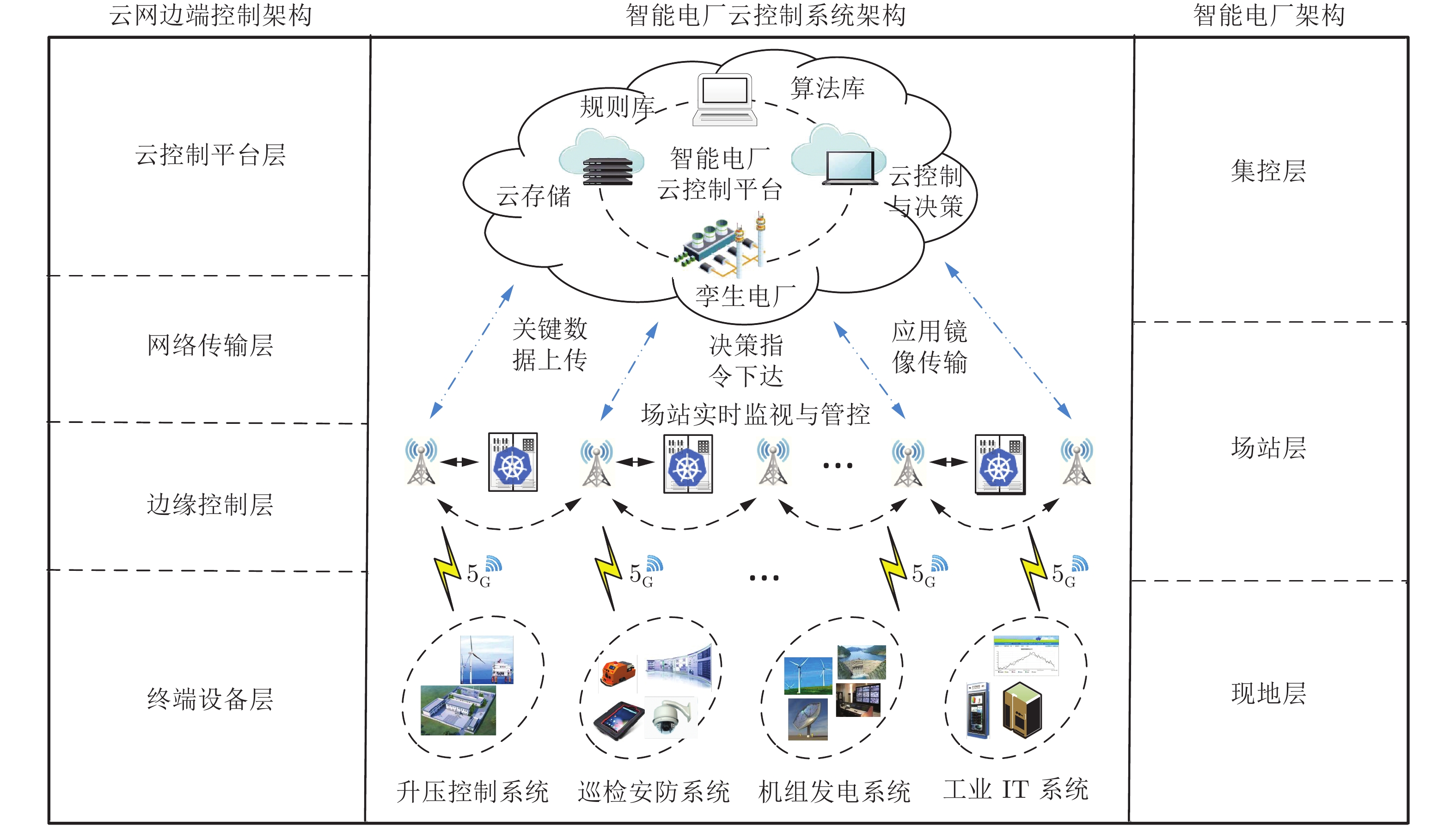
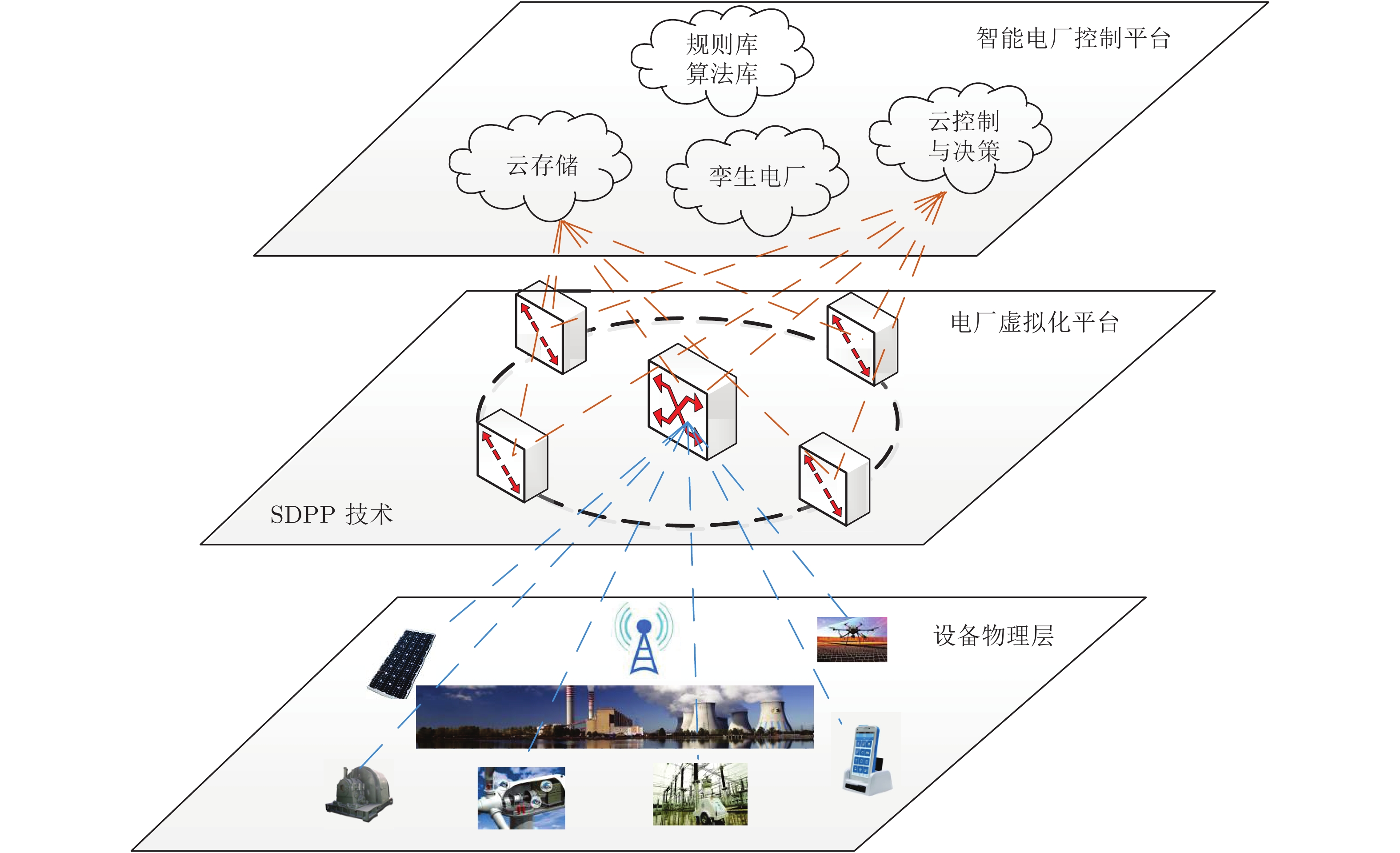
图 1 智能电厂云控制系统云网边端架构
Fig. 1 Cloud-network-edge-terminal architecture of intelligent power plant cloud control system (IPPCCS)
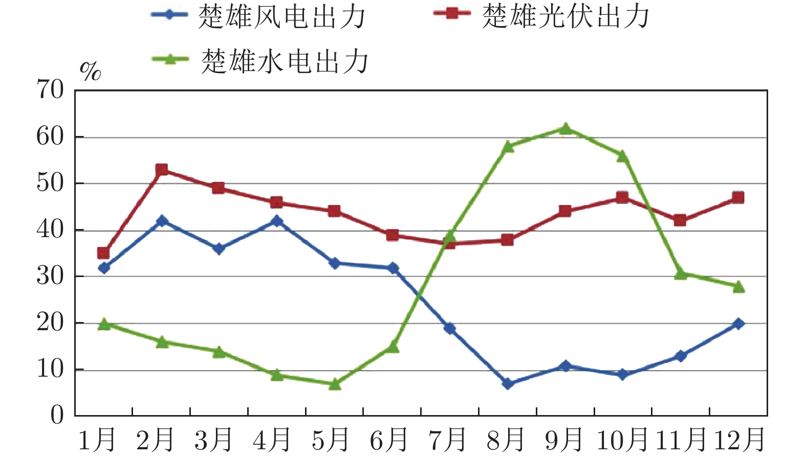
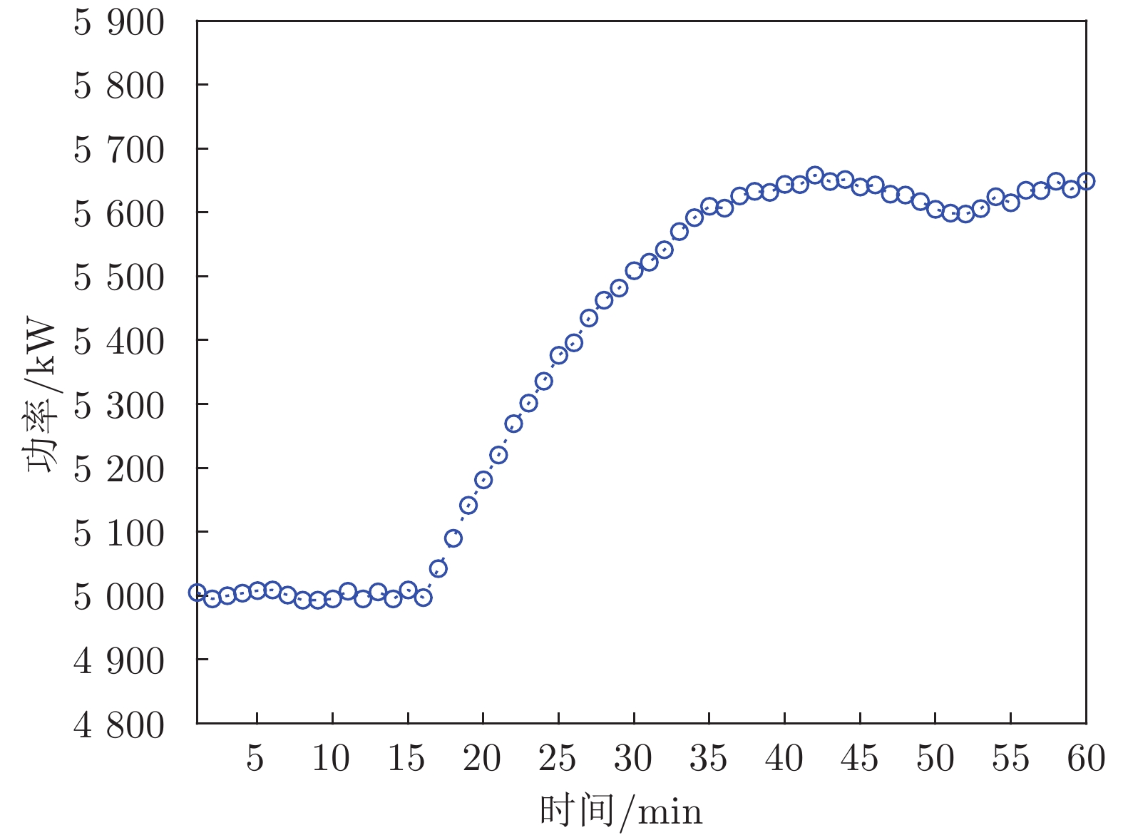
图 2 楚雄州风水光电站平均出力曲线
Fig. 2 Average output of wind, hydro and solar power in Chuxiong state

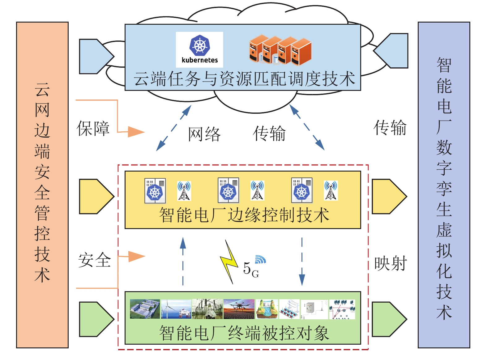
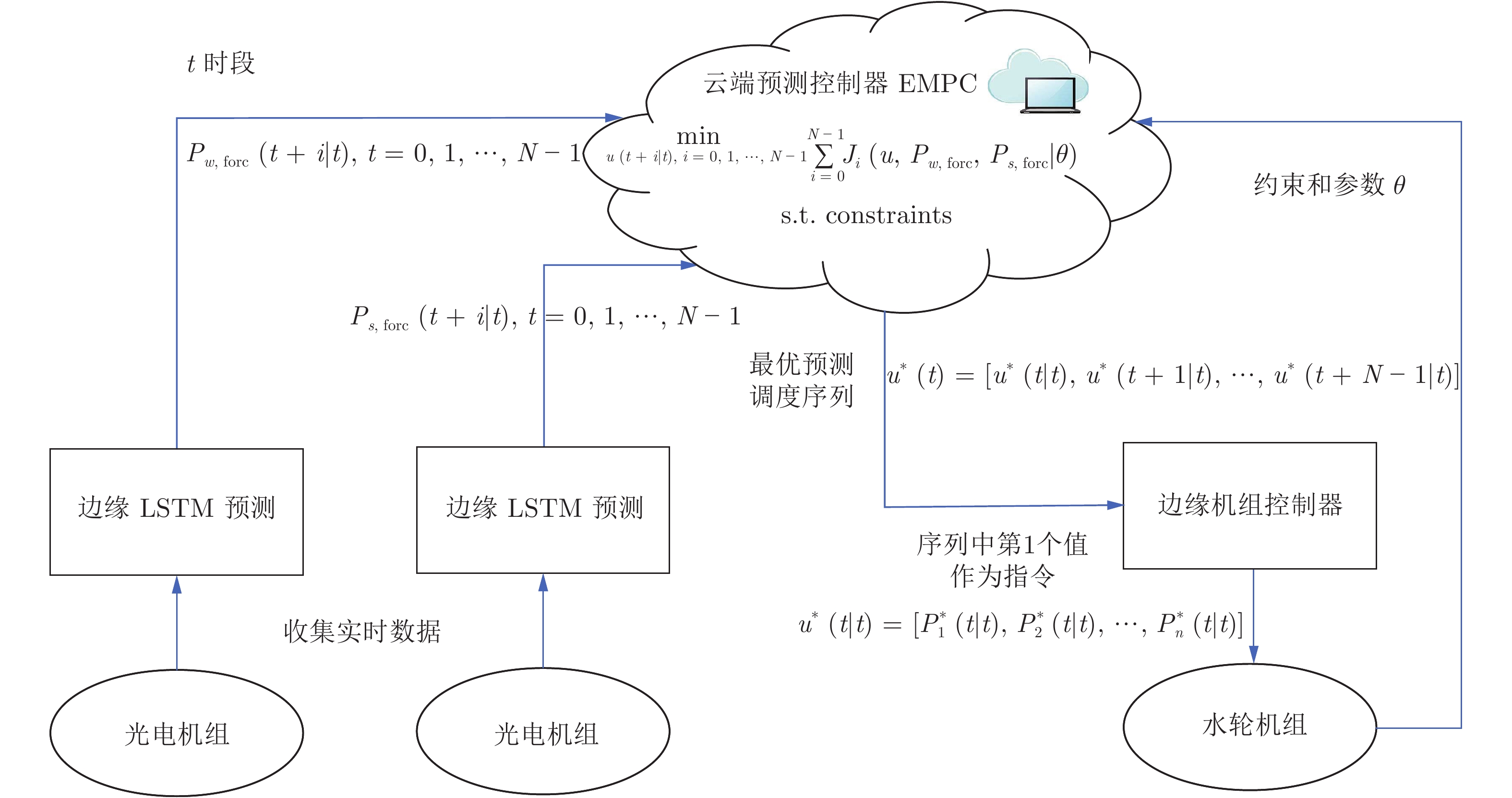
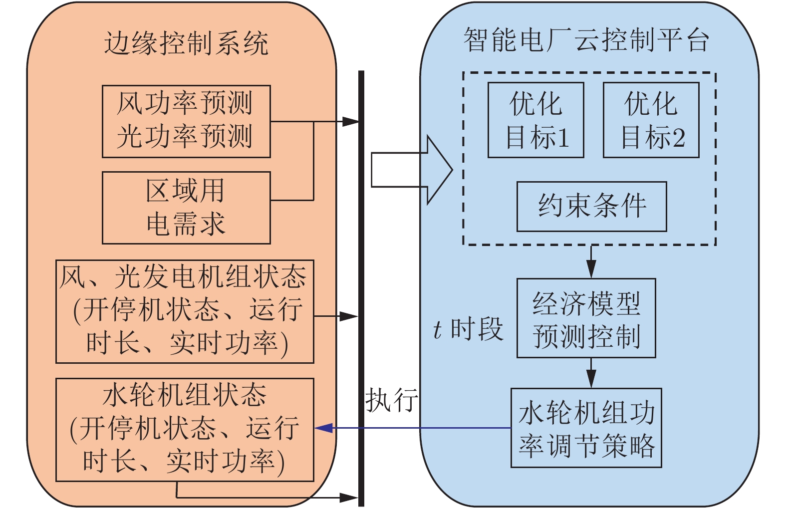
图 3 智能电厂云控制系统云边端协同控制架构
Fig. 3 Cloud-network-edge-terminal collaborative control architecture of IPPCCS
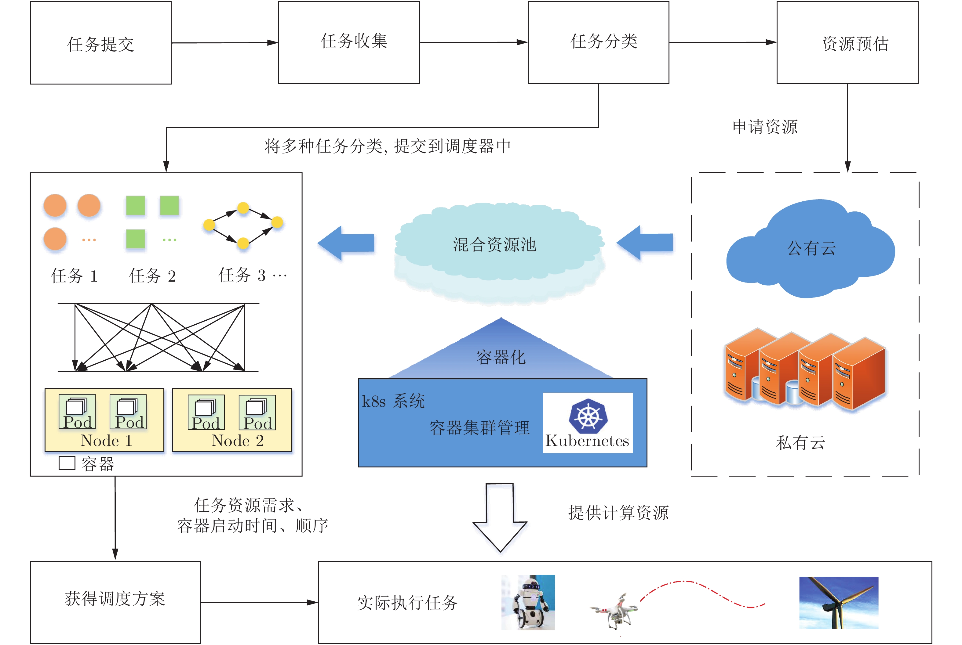
图 7 智能电厂云端任务和资源匹配调度技术框架
Fig. 7 Cloud tasks and resources matching scheduling framework in IPPCCS

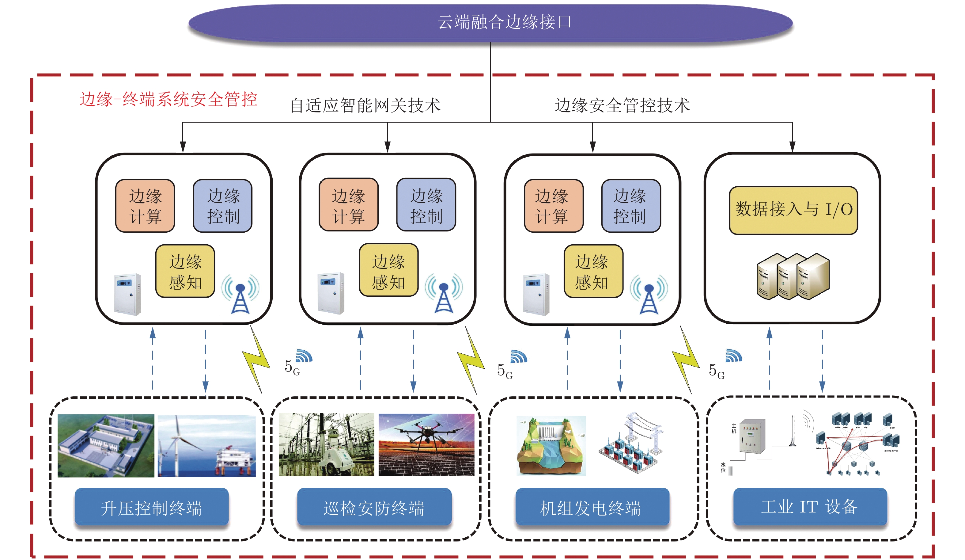
图 8 智能电厂云控制云网边端安全管控技术架构
Fig. 8 Cloud-network-edge-terminal security management and control framework in IPPCCS
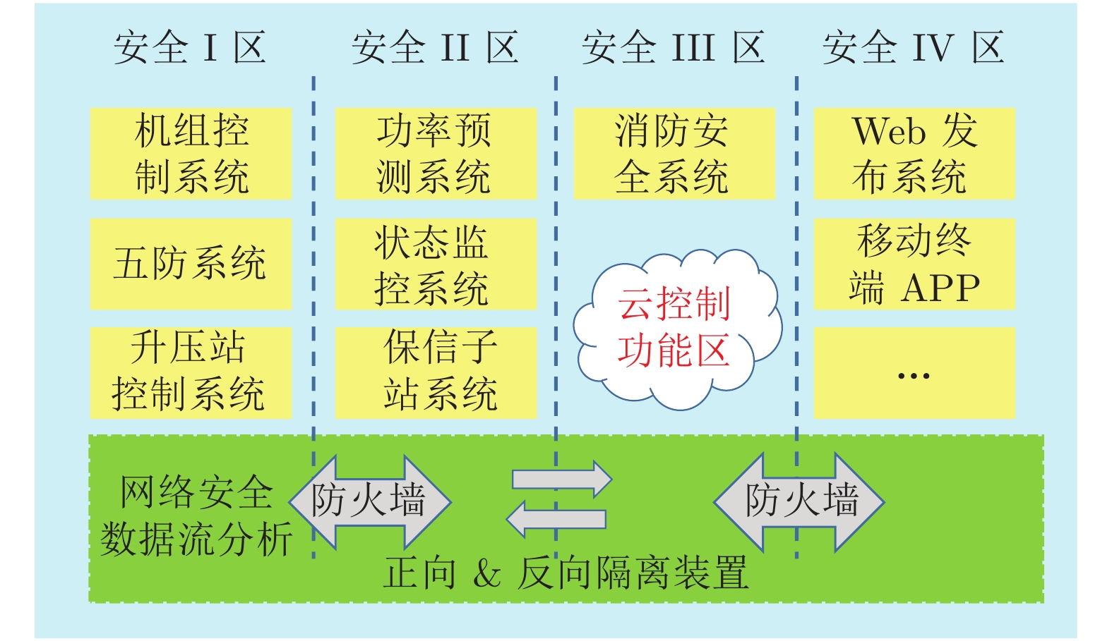
图 9 集控中心层网络安全分区业务分布图
Fig. 9 Services distribution in centralized control center for network security

图 10 含安全防护机制的云端集控中心与场站现地通信和规约方式
Fig. 10 Cloud-local communication and protocol mode with security protection mechanism
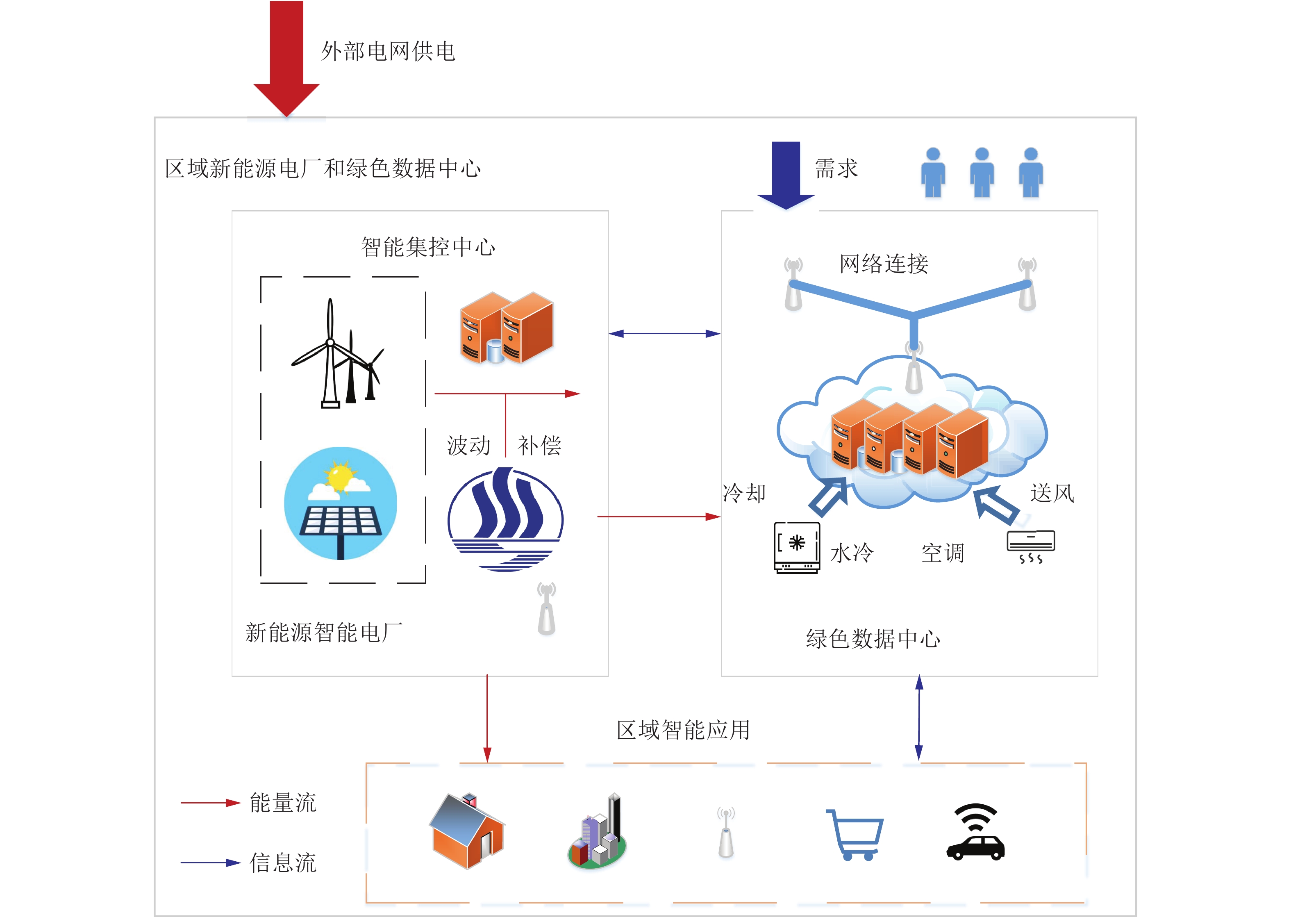
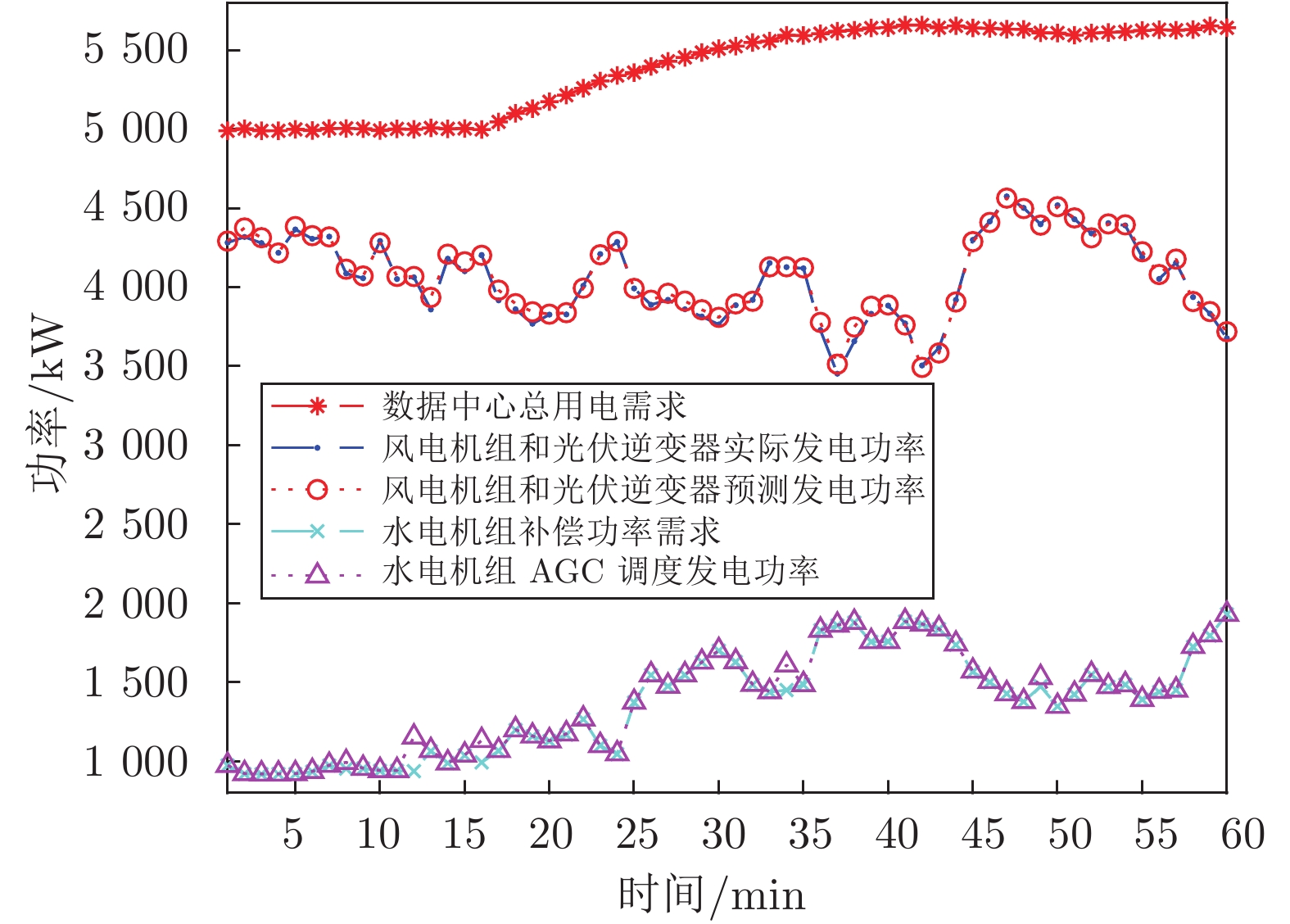
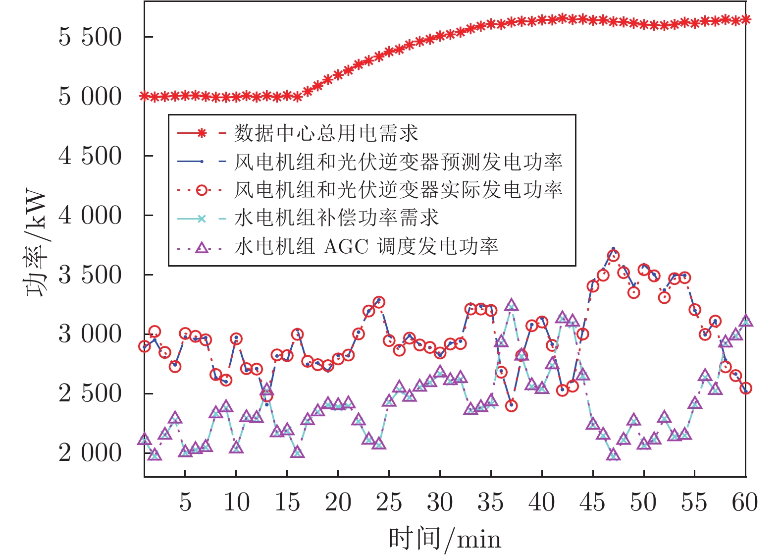
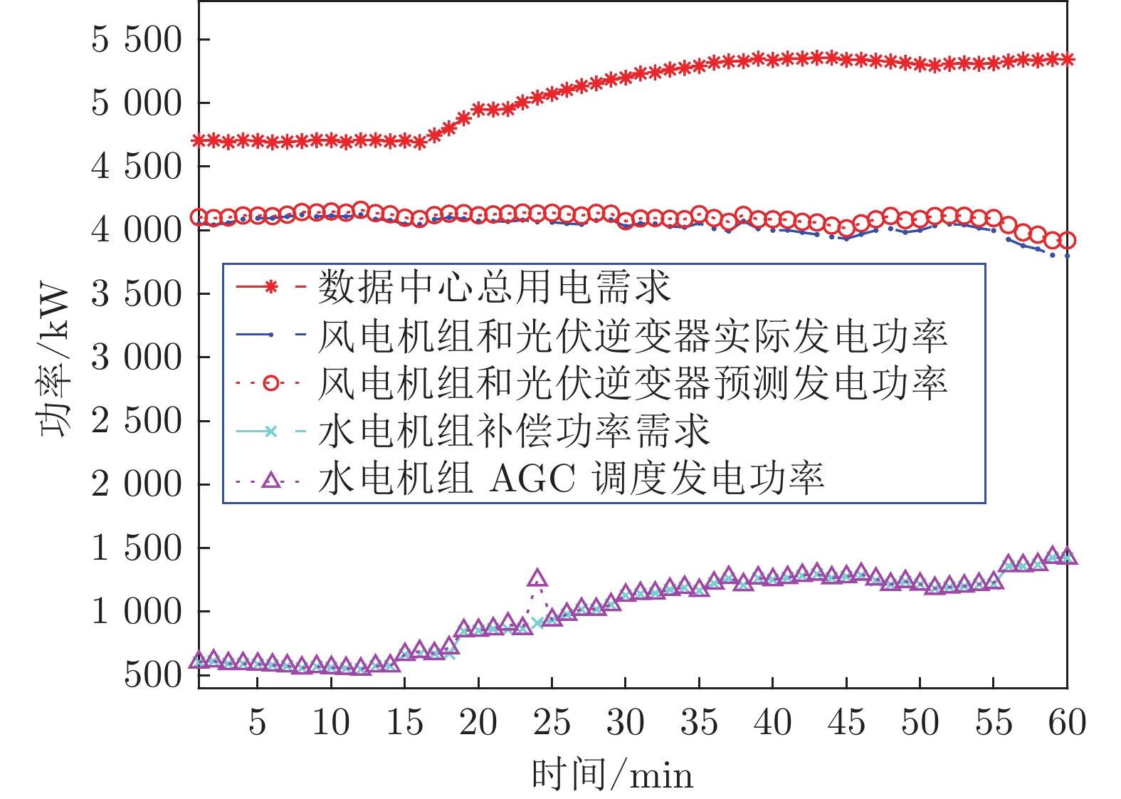
图 15 区域新能源电厂和绿色数据中心联合运行示意图
Fig. 15 Schematic diagram of joint operation of regional new energy power plant and green data center

图 16 基于LSTM网络的机组输出功率预测效果
Fig. 16 Prediction results and error rates of generators output power based on LSTM network
表 1 1号风机与1号光机未来时段预测结果
Table 1 Prediction results of No.1 wind generator and No.1 solar generator
预测时段 1号风机 1号光机 时段1 时段2 时段3 时段1 时段2 时段3 RMSE 17.383 25.569 32.469 10.703 12.787 13.645 平均误差 12.2974 19.3473 26.2758 6.2836 9.2977 11.2038 平均误差率 0.0416 0.0649 0.0878 0.0197 0.0292 0.0354  下载: 导出CSV
表 2 2 ~ 5 号风机未来时段预测结果
Table 2 Prediction results of No. 2 ~ 5 wind generators
预测时段 2号风机 3号风机 时段1 时段2 时段3 时段1 时段2 时段3 RMSE 22.869 30.357 34.298 22.842 31.128 34.999 平均误差 16.4035 23.7910 27.1607 16.4035 23.7910 27.1607 平均误差率 0.0870 0.1290 0.1489 0.0813 0.1209 0.1291 预测时段 4号风机 5号风机 时段1 时段2 时段3 时段1 时段2 时段3 RMSE 25.314 37.057 41.635 28.273 37.187 44.354 平均误差 22.0610 27.7490 33.7304 20.1751 28.2186 33.6929 平均误差率 0.0770 0.0954 0.1169 0.0696 0.0974 0.1138
下载: 导出CSV
表 3 2 ~ 5 号光机未来时段预测结果
Table 3 Prediction results of No. 2 ~ 5 solar generators
预测时段 2号光机 3号光机 时段1 时段2 时段3 时段1 时段2 时段3 RMSE 6.778 14.388 19.350 9.624 11.194 14.049 平均误差 5.5040 13.3298 16.5947 10.3386 11.2576 13.0231 平均误差率 0.0187 0.0454 0.0566 0.0333 0.0365 0.0424 预测时段 4号光机 5号光机 时段1 时段2 时段3 时段1 时段2 时段3 RMSE 9.467 9.549 14.924 7.149 8.264 17.235 平均误差 7.6231 12.4947 15.6101 8.6143 7.6891 9.6818 平均误差率 0.0242 0.0398 0.0500 0.0301 0.0272 0.0344
下载: 导出CSV
表 4 风机与光机未来时段预测平均结果
Table 4 Average results of wind and solar generators
预测时段 $1\sim 5 $ 号风机$1\sim 5 $ 号光机时段1 时段2 时段3 时段1 时段2 时段3 平均RMSE 23.336 32.260 37.551 8.744 11.236 15.841 平均误差 17.5651 24.8910 29.6411 7.6727 10.8138 13.2227 平均误差率 0.0713 0.1015 0.1193 0.0252 0.0356 0.0438
下载: 导出CSV
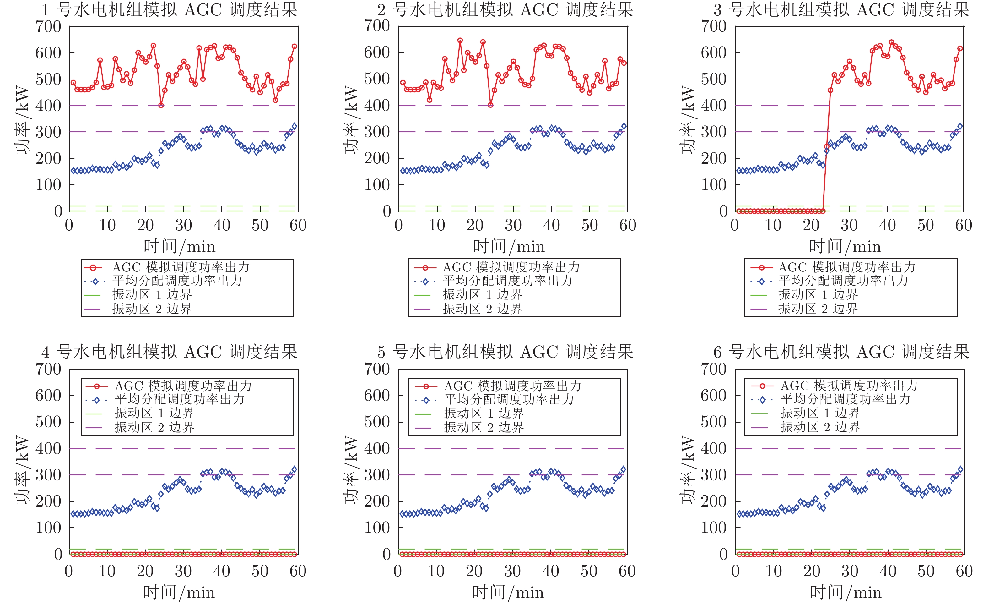
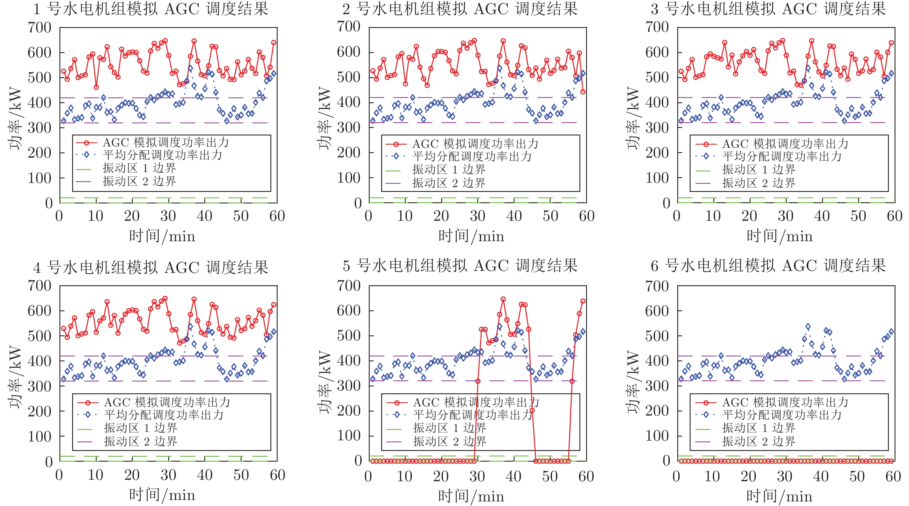
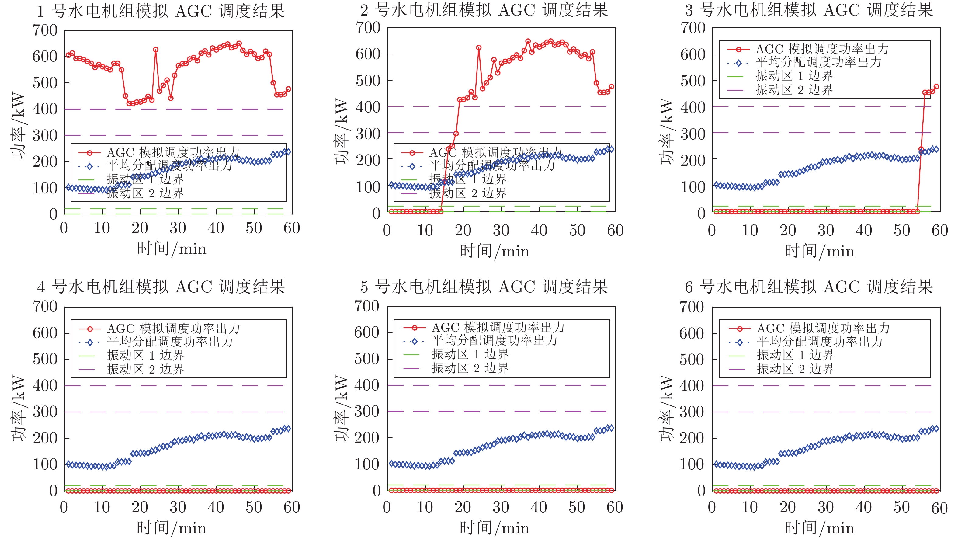
表 5 开停机和穿越振动区次数对比
Table 5 Comparison of times of on/off and crossing vibration areas
调度方式 开停机次数 穿越振动区次数 平均分配调度 6 30 AGC模拟调度 3 4
下载: 导出CSV
-
[1] Xia Y Q, Gao Y L, Yan L P, Fu M Y. Recent progress in networked control systems—a survey. International Journal of Automation and Computing, 2015, 12(4): 343−367 doi: 10.1007/s11633-015-0894-x [2] Zhang X M, Han Q L, Yu X H. Survey on recent advances in networked control systems. IEEE Transactions on Industrial Informatics, 2016, 12(5): 1740−1752 doi: 10.1109/TII.2015.2506545 [3] Wang S Y, Wan J F, Zhang D Q, Li D, Zhang C H. Towards smart factory for industry 4.0: A self-organized multi-agent system with big data based feedback and coordination. Computer Networks, 2016, 101: 158−168 doi: 10.1016/j.comnet.2015.12.017 [4] Hegazy T, Hefeeda M. Industrial automation as a cloud service. IEEE Transactions on Parallel and Distributed Systems, 2015, 26(10): 2750−2763 doi: 10.1109/TPDS.2014.2359894 [5] Xia Y Q. From networked control systems to cloud control systems. In: Proceedings of the 31st Chinese Control Conference. Hefei, China: IEEE, 2012. 5878−5883 [6] Xia Y Q. Cloud control systems. IEEE/CAA Journal of Automatica Sinica, 2015, 2(2): 134−142 doi: 10.1109/JAS.2015.7081652 [7] Xia Y Q, Qin Y M, Zhai D H, Chai S C. Further results on cloud control systems. Science China Information Sciences, 2016, 59(7): 1−5 [8] 夏元清. 云控制系统及其面临的挑战. 自动化学报, 2016, 42(1): 1−12Xia Yuan-Qing. Cloud control systems and their challenges. Acta Automatica Sinica, 2016, 42(1): 1−12 [9] 夏元清, Mahmoud M S, 李慧芳, 张金会. 控制与计算理论的交互: 云控制. 指挥与控制学报, 2017, 3(2): 99−118 doi: 10.3969/j.issn.2096-0204.2017.02.0099Xia Yuan-Qing, Mahmoud M S, Li Hui-Fang, Zhang Jin-Hui. The interaction between control and computing theories: Cloud control system. Journal of Command and Control, 2017, 3(2): 99−118 doi: 10.3969/j.issn.2096-0204.2017.02.0099 [10] Gao R Z, Xia Y Q, Ma L. A new approach of cloud control systems: CCSs based on data-driven predictive control. In: Proceedings of the 5th Chinese Automation Congress (CAC). Jinan, China: IEEE, 2017. 3419−3422 [11] Ali Y, Xia Y Q, Ma L, Hammad A. Secure design for cloud control system against distributed denial of service attack. Control Theory and Technology, 2018, 16(1): 14−24 doi: 10.1007/s11768-018-8002-8 [12] 夏元清, 闫策, 王笑京, 宋向辉. 智能交通信息物理融合云控制系统. 自动化学报, 2019, 45(1): 132−142Xia Yuan-Qing, Yan Ce, Wang Xiao-Jing, Song Xiang-Hui. Intelligent transportation cyber-physical cloud control systems. Acta Automatica Sinica, 2019, 45(1): 132−142 [13] Botta A, De Donato W, Persico V, Pescapé A. Integration of cloud computing and internet of things: A survey. Future Generation Computer Systems, 2016, 56: 684−700 doi: 10.1016/j.future.2015.09.021 [14] Shi W S, Cao J, Zhang Q, Li Y, Xu L Y. Edge computing: Vision and challenges. IEEE Internet of Things Journal, 2016, 3(5): 637−646 doi: 10.1109/JIOT.2016.2579198 [15] Thounthong P, Luksanasakul A, Koseeyaporn P, Davat B. Intelligent model-based control of a standalone photovoltaic/fuel cell power plant with supercapacitor energy storage. IEEE Transactions on Sustainable Energy, 2013, 4(1): 240−249 doi: 10.1109/TSTE.2012.2214794 [16] 刘吉臻, 胡勇, 曾德良, 夏明, 崔青汝. 智能发电厂的架构及特征. 中国电机工程学报, 2017, 37(22): 6463−6470Liu Ji-Zhen, Hu Yong, Zeng De-Liang, Xia Ming, Cui Qing-Ru. Architecture and feature of smart power generation. Proceedings of the CSEE, 2017, 37(22): 6463−6470 [17] Adhya S, Saha D, Das A, Jana J, Saha H. An IoT based smart solar photovoltaic remote monitoring and control unit. In: Proceedings of the 2nd International Conference on Control, Instrumentation, Energy and Communication (CIEC). Kolkata, India: IEEE, 2016. 432−436 [18] Zhan Z H, Liu X F, Gong Y J, Zhang J, Chung H S H, Li Y. Cloud computing resource scheduling and a survey of its evolutionary approaches. ACM Computing Surveys, 2015, 47(4): Article No. 63 [19] Qin Q F, Poularakis K, Iosifidis G, Tassulas L. SDN controller placement at the edge: Optimizing delay and overheads. In: Proceedings of the 37th Conference on Computer Communications. Honolulu, USA: IEEE, 2018. 684−692 [20] Hu L, Miao Y M, Wu G X, Hassan M, Humar I. iRobot-Factory: An intelligent robot factory based on cognitive manufacturing and edge computing. Future Generation Computer Systems, 2019, 90: 569−577 doi: 10.1016/j.future.2018.08.006 [21] 任延明. 新能源集控中心网络设计及云控制实现 [硕士学位论文], 北京理工大学, 中国, 2018.Ren Yan-Ming. Network Design and Cloud Control Implementation of New Energy Centralized Control Center [Master thesis], Beijing Institute of Technology, China, 2018. [22] 马岩岩. 大数据一体化平台在电厂中的研究与应用. 世界电信, 2017, 30(4): 64−71 doi: 10.3969/j.issn.1001-4802.2017.04.013Ma Yan-Yan. Research and application of big data integration platform in power plant. World Telecommunications, 2017, 30(4): 64−71 doi: 10.3969/j.issn.1001-4802.2017.04.013 [23] 耿清华. 浅谈基于大数据的智慧水电厂建设. 水电与新能源, 2018, 32(10): 33−35Geng Qing-Hua. Construction of the intelligent hydropower plant based on big data technology. Hydropower and New Energy, 2018, 32(10): 33−35 [24] 喻敏华. 智慧全析电厂信息平台研究与设计. 电力与能源, 2018, 39(3): 392−396, 408Yu Min-Hua. Research and design of intelligent comprehensive analysis power plant information platform. Power and Energy, 2018, 39(3): 392−396, 408 [25] Khan F A, Pal N, Saeed S H. Review of solar photovoltaic and wind hybrid energy systems for sizing strategies optimization techniques and cost analysis methodologies. Renewable and Sustainable Energy Reviews, 2018, 92: 937−947 doi: 10.1016/j.rser.2018.04.107 [26] 艾芊, 郝然. 多能互补、集成优化能源系统关键技术及挑战. 电力系统自动化, 2018, 42(4): 2−10, 46 doi: 10.7500/AEPS20170927008Ai Qian, Hao Ran. Key technologies and challenges for multi-energy complementarity and optimization of integrated energy system. Automation of Electric Power Systems, 2018, 42(4): 2−10, 46 doi: 10.7500/AEPS20170927008 [27] 赵泽. 风光水互补发电系统有功控制问题研究 [硕士学位论文]. 中国水利水电科学研究院, 中国, 2018.Zhao Ze. Research on the AGC of Complementary Power Generation Pattern of Wind Power, Solar Power and Hydropower [Master thesis], China Institute of Water Resources and Hydropower Research, China, 2018. [28] 陈丽媛, 陈俊文, 李知艺, 庄晓丹. “风光水”互补发电系统的调度策略. 电力建设, 2013, 34(12): 1−6 doi: 10.3969/j.issn.1000-7229.2013.12.001Chen Li-Yuan, Chen Jun-Wen, Li Zhi-Yi, Zhuang Xiao-Dan. Scheduling strategy of wind-photovoltaic-hydro hybrid generation system. Electric Power Construction, 2013, 34(12): 1−6 doi: 10.3969/j.issn.1000-7229.2013.12.001 [29] Taleb T, Samdanis K, Mada B, Flinck H, Dutta S, Sabella D. On multi-access edge computing: A survey of the emerging 5G network edge cloud architecture and orchestration. IEEE Communications Surveys and Tutorials, 2017, 19(3): 1657−1681 doi: 10.1109/COMST.2017.2705720 [30] Xavier M G, Neves M V, Rossi F D, Ferreto T C, Lange T, De Rose C A F. Performance evaluation of container-based virtualization for high performance computing environments. In: Proceedings of the 21st Euromicro International Conference on Parallel, Distributed, and Network-Based Processing. Belfast, United Kingdom: IEEE, 2013. 233−240 [31] Liu G P. Predictive control of networked multiagent systems via cloud computing. IEEE Transactions on Cybernetics, 2017, 47(8): 1852−1859 doi: 10.1109/TCYB.2017.2647820 [32] He X, Ju Y M, Liu Y, Zhang B C. Cloud-based fault tolerant control for a DC motor system. Journal of Control Science and Engineering, 2017, 2017(3): Article ID 5670849 [33] Li L, Wang X J, Xia Y Q, Yang H J. Predictive cloud control for multiagent systems with stochastic event-triggered schedule. ISA Transactions, 2019, 94: 70−79 doi: 10.1016/j.isatra.2019.04.011 [34] Peinl R, Holzschuher F, Pfitzer F. Docker cluster management for the cloud-survey results and own solution. Journal of Grid Computing, 2016, 14(2): 265−282 doi: 10.1007/s10723-016-9366-y [35] 罗军舟, 金嘉晖, 宋爱波, 东方. 云计算: 体系架构与关键技术. 通信学报, 2011, 32(7): 3−21 doi: 10.3969/j.issn.1000-436X.2011.07.002Luo Jun-Zhou, Jin Jia-Hui, Song Ai-Bo, Dong Fang. Cloud computing: Architecture and key technologies. Journal on Communications, 2011, 32(7): 3−21 doi: 10.3969/j.issn.1000-436X.2011.07.002 [36] Xiong Y, Sun Y L, Xing L, Huang Y. Extend cloud to edge with KubeEdge. In: Proceedings of the 2018 IEEE/ACM Symposium on Edge Computing (SEC). Seattle, WA, USA: IEEE, 2018. 373−377 [37] Haja D, Szalay M, Sonkoly B, Pongracz G, Toka L. Sharpening Kubernetes for the edge. In: Proceedings of the ACM SIGCOMM 2019 Conference Posters and Demos. Beijing, China: ACM, 2019. 136−137 [38] Majeed A A, Kilpatrick P, Spence I. Varghese B. Performance estimation of container-based cloud-to-fog offloading. arXiv: 1909.04945, 2019. [39] Tao F, Cheng J F, Qi Q L, Zhang M, Zhang H, Sui F Y. Digital twin-driven product design, manufacturing and service with big data. The International Journal of Advanced Manufacturing Technology, 2018, 94(9-12): 3563−3576 doi: 10.1007/s00170-017-0233-1 [40] Wan J F, Tang S L, Shu Z G, Li D, Wang S Y, Imran M, et al. Software-defined industrial internet of things in the context of industry 4.0. IEEE Sensors Journal, 2016, 16(20): 7373−7380 [41] Wu D, Arkhipov D I, Asmare E, Qin Z J, McCann J A. UbiFlow: Mobility management in urban-scale software defined IoT. In: Proceedings of the 34th IEEE Conference on Computer Communications. Hong Kong, China: IEEE, 2015. 208−216 [42] Chung A, Park J W, Ganger G R. Stratus: Cost-aware container scheduling in the public cloud. In: Proceedings of the 9th ACM Symposium on Cloud Computing. Carlsbad, USA: ACM, 2018. 121−134 [43] Zhang Q, Zhani M F, Boutaba R, Hellerstein J L. Dynamic heterogeneity-aware resource provisioning in the cloud. IEEE Transactions on Cloud Computing, 2014, 2(1): 14−28 doi: 10.1109/TCC.2014.2306427 [44] Bernstein D. Containers and cloud: From LXC to docker to kubernetes. IEEE Cloud Computing, 2014, 1(3): 81−84 doi: 10.1109/MCC.2014.51 [45] Zhu J, Li X P, Ruiz R, Xu X L. Scheduling stochastic multi-stage jobs to elastic hybrid cloud resources. IEEE Transactions on Parallel and Distributed Systems, 2018, 29(6): 1401−1415 doi: 10.1109/TPDS.2018.2793254 [46] Malawski M, Juve G, Deelman E, Nabrzyski J. Algorithms for cost- and deadline-constrained provisioning for scientific workflow ensembles in IaaS clouds. Future Generation Computer Systems, 2015, 48: 1−18 doi: 10.1016/j.future.2015.01.004 [47] Mao H Z, Alizadeh M, Menache I, Kandula S. Resource management with deep reinforcement learning. In: Proceedings of the 15th ACM Workshop on Hot Topics in Networks. Atlanta, USA: ACM, 2016. 50−56 [48] Yuan H H, Xia Y Q, Zhang J H, Yang H J, Mahmoud M S. Stackelberg-game-based defense analysis against advanced persistent threats on cloud control system. IEEE Transactions on Industrial Informatics, 2020, 16(3): 1571−1580 doi: 10.1109/TII.2019.2925035 [49] Zhou J, Cao Z F, Dong X L, Vasilakos A V. Security and privacy for cloud-based IoT: Challenges. IEEE Communications Magazine, 2017, 55(1): 26−33 doi: 10.1109/MCOM.2017.1600363CM [50] Manuel P. A trust model of cloud computing based on quality of service. Annals of Operations Research, 2015, 233(1): 281−292 doi: 10.1007/s10479-013-1380-x [51] Li P, Li J, Huang Z G, Li T, Gao C Z, Yiu S M, et al. Multi-key privacy-preserving deep learning in cloud computing. Future Generation Computer Systems, 2017, 74: 76−85 doi: 10.1016/j.future.2017.02.006 [52] Habib M A, Ahmad M, Jabbar S, Ahmed S H, Rodrigues J J P C. Speeding up the internet of things: LEAIoT: A lightweight encryption algorithm toward low-latency communication for the internet of things. IEEE Consumer Electronics Magazine, 2018, 7(6): 31−37 doi: 10.1109/MCE.2018.2851722 [53] Dragomir D, Gheorghe L, Costea S, Radovici A. A survey on secure communication protocols for IoT systems. In: Proceedings of the 5th International Workshop on Secure Internet of Things (SIoT). Heraklion, Greece: IEEE, 2016. 47−62 [54] Kumari S, Karuppiah M, Das A K, Li X, Wu F, Kumar N. A secure authentication scheme based on elliptic curve cryptography for IoT and cloud servers. The Journal of Supercomputing, 2018, 74(12): 6428−6453 doi: 10.1007/s11227-017-2048-0 [55] 韩璇, 袁勇, 王飞跃. 区块链安全问题: 研究现状与展望. 自动化学报, 2019, 45(1): 206−225Han Xuan, Yuan Yong, Wang Fei-Yue. Security problems on blockchain: The state of the art and future trends. Acta Automatica Sinica, 2019, 45(1): 206−225 [56] Park J, Park J. Blockchain security in cloud computing: Use cases, challenges, and solutions. Symmetry, 2017, 9(8): 164 doi: 10.3390/sym9080164 [57] Khan M A, Salah K. IoT security: Review, blockchain solutions, and open challenges. Future Generation Computer Systems, 2018, 82: 395−411 doi: 10.1016/j.future.2017.11.022 [58] Bahga A, Madisetti V K. Blockchain platform for industrial internet of things. Journal of Software Engineering and Applications, 2016, 9(10): 533−546 doi: 10.4236/jsea.2016.910036 [59] Ahmad I, Kumar T, Liyanage M, Okwuibe J, Ylianttila M, Gurtov A. Overview of 5G security challenges and solutions. IEEE Communications Standards Magazine, 2018, 2(1): 36−43 doi: 10.1109/MCOMSTD.2018.1700063 [60] 金芬兰, 王昊, 范广民, 余建明, 米为民. 智能电网调度控制系统的变电站集中监控功能设计. 电力系统自动化, 2015, 39(1): 241−247 doi: 10.7500/AEPS20141009023Jin Fen-Lan, Wang Hao, Fan Guang-Min, Yu Jian-Ming, Mi Wei-Min. Design of centralized substation monitoring functions for smart grid dispatching and control systems. Automation of Electric Power Systems, 2015, 39(1): 241−247 doi: 10.7500/AEPS20141009023 [61] Zaytar M A, El Amrani C. Sequence to sequence weather forecasting with long short-term memory recurrent neural networks. International Journal of Computer Applications, 2016, 143(11): 7−11 doi: 10.5120/ijca2016910497 [62] Rossiter J. Model-Based Predictive Control: A Practical Approach. Boca Raton: CRC Press, 2017. 52−74 [63] Müller M, Grüne L. Economic model predictive control without terminal constraints for optimal periodic behavior. Automatica, 2016, 70: 128−139 doi: 10.1016/j.automatica.2016.03.024 [64] Zong Y, Böning G M, Santos R M, You S, Hu J J, Han X. Challenges of implementing economic model predictive control strategy for buildings interacting with smart energy systems. Applied Thermal Engineering, 2017, 114: 1476−1486 doi: 10.1016/j.applthermaleng.2016.11.141 [65] 乔亮亮, 李晨坤, 付亮, 唐卫平. 某250MW水电机组振动区划分及AGC避振方法应用. 水电能源科学, 2018, 36(9): 152−154Qiao Liang-Liang, Li Chen-Kun, Fu Liang, Tang Wei-Ping. Vibration zone division of a 250MW hydropower unit and application of AGC vibration avoidance method. Water Resources and Power, 2018, 36(9): 152−154 [66] 邓维, 刘方明, 金海, 李丹. 云计算数据中心的新能源应用: 研究现状与趋势. 计算机学报, 2013, 36(3): 582−598Deng Wei, Liu Fang-Ming, Jin Hai, Li Dan. Leveraging renewable energy in cloud computing datacenters: State of the art and future research. Chinese Journal of Computers, 2013, 36(3): 582−598 [67] 温正楠, 刘继春. 风光水互补发电系统与需求侧数据中心联动的优化调度方法. 电网技术, 2019, 43(7): 2449−2459Wen Zheng-Nan, Liu Ji-Chun. A optimal scheduling method for hybrid wind-solar-hydro power generation system with data center in demand side. Power System Technology, 2019, 43(7): 2449−2459 -

 下载:
下载:


计量
- 文章访问数: 2747
- HTML全文浏览量: 1111
- PDF下载量: 435
- 被引次数: 0
