2.845

2023影响因子

(CJCR)

  • 中文核心
  • EI
  • 中国科技核心
  • Scopus
  • CSCD
  • 英国科学文摘

留言板

尊敬的读者、作者、审稿人, 关于本刊的投稿、审稿、编辑和出版的任何问题, 您可以本页添加留言。我们将尽快给您答复。谢谢您的支持!

姓名
邮箱
手机号码
标题
留言内容
验证码

基于事件相机的定位与建图算法: 综述

马艳阳 叶梓豪 刘坤华 陈龙

张檬,  韩敏.  基于单向耦合法的不确定复杂网络间有限时间同步.  自动化学报,  2021,  47(7): 1624−1632 doi: 10.16383/j.aas.c180102
引用本文: 马艳阳,  叶梓豪,  刘坤华,  陈龙.  基于事件相机的定位与建图算法: 综述.  自动化学报,  2021,  47(7): 1484−1494 doi: 10.16383/j.aas.c190550
Zhang Meng,  Han Min.  Finite-time synchronization between uncertain complex networks based on unidirectional coupling method.  Acta Automatica Sinica,  2021,  47(7): 1624−1632 doi: 10.16383/j.aas.c180102
Citation: Ma Yan-Yang,  Ye Zi-Hao,  Liu Kun-Hua,  Chen Long.  Event-based visual localization and mapping algorithms: a survey.  Acta Automatica Sinica,  2021,  47(7): 1484−1494 doi: 10.16383/j.aas.c190550

基于事件相机的定位与建图算法: 综述

doi: 10.16383/j.aas.c190550
基金项目: 国家重点研发计划(2018YFB1305002), 国家自然科学基金(61773414)资助
详细信息
    作者简介:

    马艳阳:2020年获得中山大学硕士学位. 2018年获得中山大学计算机科学与技术学士学位. 主要研究方向为机器人定位与建图技术. E-mail: mayany3@mail2.sysu.edu.cn

    叶梓豪:中山大学计算机学院硕士研究生. 2020年获得中山大学软件工程学士学位. 主要研究方向为多传感器融合的即时同步定位与建图技术. E-mail: yezh9@mail2.sysu.edu.cn

    刘坤华:中山大学数据科学与计算机学院博士后. 2019年获得山东科技大学机电工程学院博士学位. 主要研究方向为自动驾驶环境感知. E-mail: lkhzyf@163.com

    陈龙:中山大学数据科学与计算机学院副教授. 于2007年、2013年获得武汉大学学士、博士学位. 主要研究方向为自动驾驶, 机器人, 人工智能. 本文通信作者. E-mail: chenl46@mail.sysu.edu.cn

Event-based Visual Localization and Mapping Algorithms: A Survey

Funds: Supported by National Key Research and Development Program of China (2018YFB1305002), National Natural Science Foundation of China (61773414)
More Information
    Author Bio:

    MA Yan-Yang He received his master degree from the School of Computer Science and Engineering, Sun Yat-Sen University in 2020. He received his bachelor degree from Sun Yat-Sen University in 2018. His research interest covers robot localization and mapping

    YE Zi-Hao Master student at the School of Computer Science and Engineering, Sun Yat-Sen University. He received his bachelor degree in software engineering from Sun Yat-Sen University in 2020. His research interest covers real-time synchronous localization and mapping technology of multi-sensor fusion

    LIU Kun-Hua Postdoctor at the School of Data and Computer Science, Sun Yat-sen University. She received her Ph.D. degree from the Mechanical and Electrical Engineering Institute, Shandong University of Science and Technology. Her research interest covers automatic driving environment perception

    CHEN Long Associate professor at the School of Data and Computer Science, Sun Yat-sen University. He received his bachelor degree and Ph.D. degree from Wuhan University in 2007 and 2013. His research interest covers autonomous driving, robotics and artificial intelligence. Corresponding author of this paper

  • 摘要:

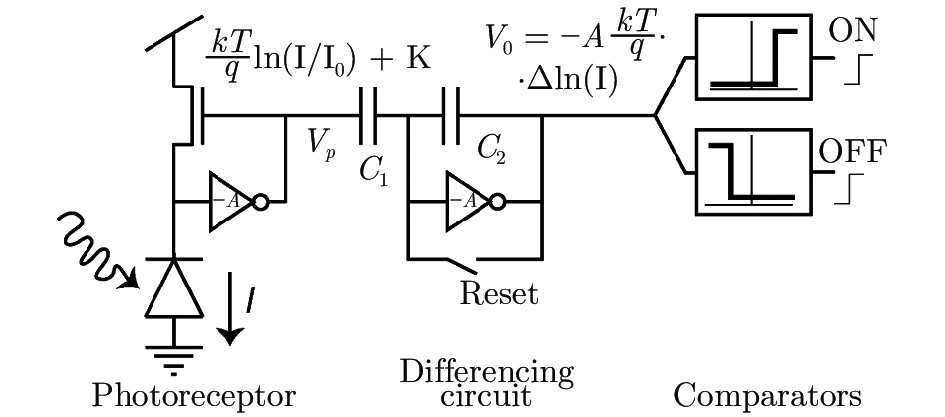
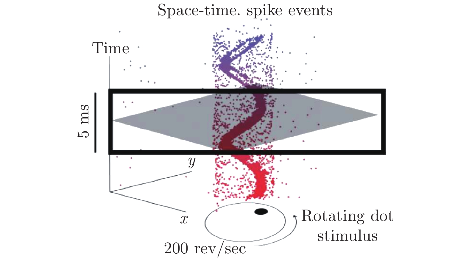
    事件相机是一种新兴的视觉传感器, 通过检测单个像素点光照强度的变化来产生“事件”. 基于其工作原理, 事件相机拥有传统相机所不具备的低延迟、高动态范围等优良特性. 而如何应用事件相机来完成机器人的定位与建图则是目前视觉定位与建图领域新的研究方向. 本文从事件相机本身出发, 介绍事件相机的工作原理、现有的定位与建图算法以及事件相机相关的开源数据集. 其中, 本文着重对现有的、基于事件相机的定位与建图算法进行详细的介绍和优缺点分析.

  • 机动目标跟踪(Maneuvering target tracking, MTT)是状态估计领域的重要研究方向之一, 广泛应用于雷达跟踪、飞行目标监测、导航等领域. 目前机动目标跟踪方法的研究主要基于卡尔曼滤波(Kalman filter, KF). 卡尔曼滤波是一种基于先验模型的估计方法, 要求先验模型准确, 即目标运动模式已知. 然而, 机动目标的机动性就体现在其运动模式未知且剧烈变化, 因此单模型方法难以有效解决机动目标跟踪问题. 基于多模型的跟踪方法是目前机动目标跟踪的重要研究领域. 以交互式多模型(Interacting multiple model, IMM)[1]为代表的多模型机动目标跟踪方法结合隐马尔科夫模型(Hidden Markov models, HMM), 利用模型转移概率提高对机动目标的状态估计精度. IMM方法采用模型集, 但Li认为实际模式空间与模型集合不一定匹配, 且模型集合应适应外界条件变化, 并提出变结构多模型方法(Variable structure multiple model, VSMM)[2-5]. 由于其良好的状态估计效果和灵活性, VSMM方法被国内外学者广泛关注.

    随着传感器、计算机和通信技术发展, 多传感器信息融合逐渐成为研究热点, 可分为集中式(Centralized)、分布式(Distributed)与混合式(Hierarchical) 三种融合架构[6]. 基于一致性的分布式融合架构无需融合中心, 具有通信带宽要求低、通信能量损耗低、且对复杂网络适应性强等优点, 日益受到国内外学者关注. 基于一致性的分布式状态估计包括多种实现形式, 例如卡尔曼一致滤波(Kalman consensus filter, KCF)[7-9]、信息一致滤波(Information consensus filter, ICF)[10-11]等.

    目前对一致性滤波的研究主要基于单模型方法, 主要关注传感器网络内丢包[12]、时延[13]、动态网络拓扑[14]、自适应一致性滤波[15]、网络能量优化[16]以及带牵引控制[17]等问题. 近年来, 考虑到多模型方法比单模型方法有更好的机动目标跟踪效果, Chisci等学者结合多模型思想, 提出分布式交互式多模型估计方法 (Distributed interacting multiple model, DIMM)[18-20]. 虽然变结构交互式多模型比交互式多模型具有更好的跟踪精度, 但由于VSMM方法中模型集随时可能扩增或删减, 难以直接应用于基于一致性的分布式估计方法, 因此目前已发表的相关研究成果不多.

    本文重点研究如何将变结构多模型方法有效地引入分布式非线性状态估计方法, 具体研究内容如下: 首先为了解决量测方程非线性的问题, 研究了一类无迹信息滤波方法(Unscented information filter, UIF); 通过对变结构多模型方法进行改进, 提出基于可能模型集的期望模式扩增方法 (Expected-mode augmentation based on likely model-set, EMA-LMS), 进而将VSMM应用于分布式状态估计, 提出分布式变结构多模型方法 (Distributed variable structure multiple model, DVSMM). 仿真实验结果验证了本文提出方法的有效性.

    本节介绍分布式传感器网络的图论表示以及雷达和红外传感器的量测模型.

    通常用图$G = (V,E)$对传感器网络建模. 顶点集$V = \{ 1,2,\cdots,n\}$表示网络中的传感器节点. 如果传感器节点$i$$j$可以通信, 则认为图中这两个节点之间存在边, 即$(i,j) \in E$. 邻接矩阵${A}$$n$$n$列的布尔矩阵, 记${A} = [{a_{ij}}]$, 如式1所示:

    $${a_{ij}} = \left\{ \begin{array}{l} 1,\hskip5mm{\rm{ (}}i,j) \in E\\ 0,\hskip5mm{\rm{ (}}i,j) \notin E{\rm{\ or\ }}i = j \end{array} \right.$$ (1)

    ${N_i} = \{ j:({v_i},{v_j}) \in E\} $为传感器节点$i$可以通通信的节点集, ${J_i} = {N_i} \cup \{ i\} $. 如图1所示: 包含6节点的分布式传感器网络.

    图 1  用无向图表示的传感器网络
    Fig. 1  A sensor network expressed by undirected graph

    该传感器网络对应的邻接矩阵如式(2)所示:

    $${A} = \left[ {\begin{array}{*{20}{c}} 0&1&0&1&1&1 \\ 1&0&1&0&0&1 \\ 0&1&0&1&0&0 \\ 1&0&1&0&1&0 \\ 1&0&0&1&0&1 \\ 1&1&0&0&1&0 \end{array}} \right]$$ (2)

    本文研究二维平面内直接坐标系中的机动目标跟踪问题. 记视线与直角坐标系$x$轴正方向的夹角记为方位角$\theta, $ 传感器与目标的距离记为$\rho.$ 雷达可获得目标距离$\rho $与方位角$\theta $量测值, 而红外传感器仅获得目标方位角$\theta,$图2所示.

    图 2  雷达和红外传感器量测模型
    Fig. 2  Measurement model of radar and infrared

    构造极坐标$(\rho ,\theta )$与二维平面上直角坐标描述$(x,y)$一一映射, 如式(3)所示, 方位角的范围须为$\theta \in [0,2\pi )$$\theta \in ( - \pi ,\pi ]$:

    $$\left\{ \begin{array}{l} x = \rho \cos \theta \\ y = \rho \sin \theta \end{array} \right.$$ (3)

    $\theta \in [0,2\pi )$时, 直角坐标$(x,y)$转换为极坐标$(\rho ,\theta )$的映射关系如式(4)所示.

    $$\begin{split} &\rho = \sqrt {{{({x_t} - {x_s})}^2} + {{({y_t} - {y_s})}^2}} \\ &\theta = \left\{ \begin{aligned} &\arctan \frac{{{y_t} - {y_s}}}{{{x_t} - {x_s}}},\ {\rm{ }}{x_t} - {x_s} > 0,\ {y_t} - {y_s} \ge 0\\ &\arctan \frac{{{y_t} - {y_s}}}{{{x_t} - {x_s}}} + 2\pi ,\ {\rm{ }}{x_t} - {x_s} > 0,\ {y_t} - {y_s} < 0\\ &\arctan \frac{{{y_t} - {y_s}}}{{{x_t} - {x_s}}} + \pi ,\ {\rm{ }}{x_t} - {x_s} < 0\\ &\frac{\pi }{2},\ {\rm{ }}{x_t} - {x_s} = 0{\rm{,\ }}{y_t} - {y_s} > 0\\ &\frac{{3\pi }}{2},\ {\rm{ }}{x_t} - {x_s} = 0{\rm{,\ }}{y_t} - {y_s} < 0 \end{aligned} \right. \end{split}$$ (4)

    式中, ${x_t}$${y_t}$表示目标位置; ${x_s}$${y_s}$表示传感器位置. 式(4)中的映射关系不具有连续性, 即存在一组由奇异点构成射线$y = 0,\ x > 0.$ 且目标方位角在该射线两侧发生突变, 导致目标方位角误差增大, 影响滤波器的状态估计结果.

    为避免由反正切函数不连续引起的误差, 需判断映射关系是否奇异.

    图 3  $ {\theta }_{1}-{\theta }_{2} $的定义
    Fig. 3  Definition of $ {\theta }_{1}-{\theta }_{2} $

    首先计算相邻两个时刻目标方位角的顺时针变量$\Delta {\theta _{acw}}$与逆时针变量$\Delta {\theta _{cw}}$, 构造具有连续性的映射关系, 如式(5)所示, 计算方位角的变化量.

    $$\begin{split} {\theta _1} - {\theta _2} =\;& \left\{ {\begin{aligned} &{0,} \qquad\qquad\;\; {{\theta _1} - {\theta _2} = 0}\\ &{\Delta {\theta _{acw}},} \;\qquad {\Delta {\theta _{cw}} > \Delta {\theta _{acw}}}\\ &{ - \Delta {\theta _{cw}},}\qquad {\Delta {\theta _{cw}} < \Delta {\theta _{acw}}} \end{aligned}} \right.=\\ \;&\left\{ {\begin{aligned} &{{\theta _1} - {\theta _2},}\;\;\;\qquad\qquad{\left| {{\theta _1} - {\theta _2}} \right| \le \pi }\\ &{2\pi - \left| {{\theta _1} - {\theta _2}} \right|,}\qquad{{\theta _1} - {\theta _2} < - \pi }\\ &{\left| {{\theta _1} - {\theta _2}} \right| - 2\pi ,}\;\qquad{{\theta _1} - {\theta _2} > \pi } \end{aligned}} \right. \end{split}$$ (5)

    本节介绍下一节中DVSMM方法所采用的无迹信息滤波UIF[21]原理. 无迹信息滤波与无迹卡尔曼滤波 (Unscented Kalman filter, UKF) 均通过Sigma点采样计算状态向量的一阶矩与二阶矩, 区别在于UIF采用信息矩阵与信息状态向量进行量测更新.

    $x$n维随机向量, 其均值和协方差分别为$\bar x$${{P}_x}$. ${{f}} ( \cdot )$为非线性函数:

    1)计算$2n + 1$个Sigma点${\xi ^\iota }$:

    $$\left\{ \begin{aligned} &{\xi ^i} = \bar x,{\rm{ }}\ i = 0\\ &{\xi ^i} = \bar x + {(\sqrt {(n + \lambda ){P_x}} )_i}{\rm{, }}\ i = 1,\cdots,n\\ &{\xi ^i} = \bar x - {(\sqrt {(n + \lambda ){P_x}} )_{i - n}}{\rm{, }}\ i = n + 1,\cdots,2n \end{aligned} \right.$$ (6)

    式中, $\lambda $为尺度参数; ${(\sqrt {(n + \lambda ){P_x}} )_i}$表示用$(n + \lambda ){{P}_x}$平方根的第$i$行或第$i$列来构造Sigma点[22-24].

    2)每个Sigma点通过非线性函数传播, 得到${y^i}$:

    $${y^i} = f({\xi ^i}),\quad {\rm{ }}i = 0,\cdots,2n$$ (7)

    3)计算$y$的均值$\bar y$和协方差${{P}_y}$.

    $$\begin{split} &\bar y = \sum\limits_{i = 0}^{2n} {W_s^i{y^i}} \\ &{{P}_y} = \sum\limits_{i = 0}^{2n} {W_c^i({y^i} - \bar y){{({y^i} - \bar y)}^{\rm{T}}}} \end{split}$$ (8)

    式中, $W_s^i$$W_c^i$为加权系数[22-23].

    设离散时间非线性系统的状态方程和量测方程如式(9)所示:

    $$\begin{split} &{x_k} = {f_{k - 1}}({x_{k - 1}}) + {w_k}\\ &{z_k} = {h_k}({x_k}) + {v_k} \end{split}$$ (9)

    式中, ${x_k}$表示目标状态向量; ${z_k}$表示传感器量测向量; ${{f}}_{k}(\cdot )$${{h}}_{k}(\cdot )$分别表示非线性的状态函数和量测函数; ${w_k} \sim {\rm N}(0,{{Q}_k})$表示过程噪声; ${v_k} \sim {\rm N}(0,{{R}_k})$表示量测噪声.

    假设上一时刻的状态估计${\hat x_{k \!-\! 1|k \!-\! 1}}$和估计协方差矩阵${{P}_{k - 1|k - 1}}$已知, 状态向量维度为$L,$ 量测向量维度为$M.$ 则UIF的一步状态预测与量测更新过程如下:

    1)一步状态预测

    由式(6), 计算${\hat x_{k - 1|k - 1}}$周围的Sigma点$x_{k - 1|k - 1}^i$, $i = 0,1,\cdots,2L.$ 计算$x_{k - 1|k - 1}^i$经过状态转移函数${{f}}_{k-1}( \cdot )$传递后的$x_{k|k - 1}^i.$ 由式(10)计算状态预测${\hat x_{k|k - 1}}$和状态预测协方差${P_{k|k - 1}}:$

    $$\begin{split} &{{\hat x}_{k|k - 1}} = \sum\limits_{i = 0}^{2n} {W_s^ix_{k|k - 1}^i} \\ &{{P}_{k|k - 1}} = \sum\limits_{i = 0}^{2n} W_c^i(x_{k|k - 1}^i - {{\hat x}_{k|k - 1}})\times\\ &\qquad\qquad{(x_{k|k - 1}^i - {\hat x}_{k|k - 1}})^{\rm T} + {{Q}_k} \end{split}$$ (10)

    计算先验信息向量${\hat y_{k|k - 1}}$和对应的信息矩阵${{Y}_{k|k - 1}}$:

    $$\begin{split} &{{\hat y}_{k|k - 1}} = {P}_{k|k - 1}^{ - 1}{{\hat x}_{k|k - 1}}\\ &{{Y}_{k|k - 1}} = {P}_{k|k - 1}^{ - 1} \end{split}$$ (11)

    2)量测更新

    计算$x_{k|k - 1}^i$在量测函数下的映射$g_k^i$:

    $$g_k^i = {{h}_k}(x_{k|k - 1}^i),\;\;\;i = 0,1,\cdots,2L$$ (12)

    计算量测预测${\hat z_k}$:

    $${\hat z_k} = \sum\limits_{i = 0}^{2L} {W_s^ig_k^i} $$ (13)

    计算量测预测和状态−量测协方差矩阵:

    $$\begin{split} &{{P}_{{z_k}{z_k}}} = \sum\limits_{i = 0}^{2L} {W_c^i(g_k^i - {{\hat z}_k}){{(g_k^i - {{\hat z}_k})}^{\rm{T}}}} + {{R}_k}\\ &{{P}_{{x_k}{z_k}}} = \sum\limits_{i = 0}^{2L} {W_c^i(x_{k|k - 1}^i - {{\hat x}_{k|k - 1}}){{(g_k^i - {{\hat z}_k})}^{\rm{T}}}} \end{split}$$ (14)

    引入伪测量矩阵计算信息状态贡献${i_k}$和对应的信息矩阵${I_k}$[21]:

    $$\begin{split} {{I}_k} =\;& {P}_{k|k{\rm{ - 1}}}^{{\rm{ - 1}}}{{P}_{{x_k}{z_k}}}{R}_k^{{\rm{ - 1}}}{P}_{{x_k}{z_k}}^{\rm{T}}{P}_{k|k{\rm{ - 1}}}^{{\rm{ - 1}}}\\ {i_k} =\;& {P}_{k|k{\rm{ - 1}}}^{{\rm{ - 1}}}{{P}_{{x_k}{z_k}}}{R}_k^{{\rm{ - 1}}}{\rm{\bigg(}}{z_k} - {{\hat z}_k} +\\ &{P}_{{x_k}{z_k}}^{\rm{T}}{\left({P}_{k|k{\rm{ - 1}}}^{\rm{T}}\right)^{{\rm{ - 1}}}}{{\hat x}_{k|k{\rm{ - 1}}}}\bigg) \end{split}$$ (15)

    通过${i_k}$${{I}_k}$计算后验信息向量${\hat y_{k|k}}$和对应的信息矩阵${{Y}_{k|k}}$:

    $$\begin{split} &{{Y}_{k|k}} = {{Y}_{k|k - 1}} + {{I}_k}\\ &{{\hat y}_{k|k}} = {{\hat y}_{k|k - 1}} + {i_k} \end{split}$$ (16)

    由式(17)计算状态估计${\hat x_{k|k}}$和状态估计协方差${P_{k|k}}$:

    $$\begin{split} &{{P}_{k|k}} = {Y}_{k|k}^{ - 1}\\ &{{\hat x}_{k|k}} = {Y}_{k|k}^{ - 1}{{\hat y}_{k|k}} \end{split}$$ (17)

    考虑到第1.2节所述的方位角突变的问题, 需要按照如下两个步骤修改UIF:

    将式(13)改为直接用${\hat x_{k|k - 1}}$来计算${\hat z_k}$:

    $${\hat z_k} = {{h}_k}({\hat x_{k|k - 1}})$$ (18)

    将式(14)、(15)中$g_k^i - {\hat z_k}$${z_k} - {\hat z_k}$中的方位角相减都用式(5)的角度相减代替.

    本节将分析变结构多模型方法应用在分布式状态估计所面临的关键问题. 通过结合期望模式扩增方法和可能模型集方法, 提出基于可能模型集的期望模式扩增方法 EMA-LMS与分布式变结构多模型跟踪方法DVSMM.

    在DIMM[18-20]方法框架下, 将每个模型对应的预测信息或传感器后验估计信息与通信邻域中其他传感器对应模型中的信息进行一致性加权融合, 如图4所示:

    图 4  交互模型预测信息的DIMM方法示意图
    Fig. 4  Diagram of DIMM with mode-matched PDFs

    图4中, 每个传感器具有相同的交互式多模型集, 且模型数量为$M.$ 假设传感器$s$$j$相邻, 本地传感器与相邻传感器进行一致性加权融合的变量可分为三类: 1)本地先验信息向量${\hat y_{k|k - 1}}$及其对应的信息矩阵${{Y}_{k|k - 1}};$ 2)本地信息状态贡献${i_k}$和对应的信息矩阵${{I}_k}$[18]; 3)本地后验信息向量${\hat y_{k|k}}$和对应的信息矩阵${{Y}_{k|k}}$[19]. 此外, 分布式交互式多模型方法将对每个模型下的模型似然对数与相邻传感器对应模型下的模型似然对数进行一致性加权融合[18].

    但上述DIMM方法框架并不适用于分布式变结构交互式多模型方法. VSMM方法中不同时刻模型集的模型种类与数量可能不同. 即在每个方法周期内, 每个传感器所使用的模型可能不一样. 因此实现分布式VSMM方法主要有面临两个难点:

    1) 信息滤波器中先验及后验的信息向量${y_k}$、对应的信息矩阵${{Y}_k}$和多模型方法中的模型似然都依赖于模型和传感器本地量测向量${z_k}$来计算. 由于VSMM方法每个时刻使用的模型种类和数量都在变化, 因此无法像分布式IMM方法那样对每个模型对应的这些信息使用一致性加权融合.

    2) 在线性系统中与非线性系统中, 信息状态贡献${i_k}$和对应的信息矩阵${{I}_k}$的计算不但依赖于本地量测${z_k}$, 也依赖于模型.

    图5所示, 每个传感器每个时刻所交互的模型不同(VSMM方法核心特点), 因此无法采用DIMM方法的思路实现分布式状态估计.

    图 5  分布式变结构多模型方法面临难题
    Fig. 5  The difficulty in achieving DVSMM

    由于VSMM方法在不同时刻选用不同的模型集进行交互, 因此难以在相邻传感器之间直接交互模型的信息向量和信息矩阵. 为解决这一问题, 本文对Li提出的VSMM方法结合无迹信息滤波UIF进行改进, 提出分布式变结构多模型跟踪方法(DVSMM). 通过在相邻传感器之间直接传递量测向量, 并在每个传感器内部平行计算采用不同模型的UIF对应的信息向量、信息矩阵和模型似然函数, 最后进行一致性加权融合. DVSMM具体方法如下:

    假设本地传感器为传感器$s$, 通过MSA方法可得$k$时刻本地用于状态估计的新模型集合$M_k^s$. 假设每个方法周期开始时, 每个传感器已经向相邻的传感器发送本时刻自身的本地量测${z_k}$和位置${p_k}$, 且每个传感器可知其他传感器量测向量来自的传感器类型(雷达或红外). 记${J_s} = {N_s} \cup \{ s\} $, 则传感器$s$在本方法周期可用的传感器量测为$\{ z_k^m\} ,m \in {J_s}$.

    对模型$i$, 目标的状态转移方程为:

    $${x_k} = f_{k - 1}^{(i)}({x_{k - 1}}) + w_k^{(i)}$$ (19)

    式中, $w_k^{(i)}$为过程噪声, $w_k^{(i)} \sim {\rm N}(0,{Q}_k^{(i)})$.

    传感器$s$的量测方程为:

    $$z_k^s = {h}_k^s({x_k}) + v_k^s$$ (20)

    式中, $v_k^s$为量测噪声, $v_k^s \sim {\rm N}(0, R_k^s)$.

    假设$ k-1 $时刻基于$M_{k - 1}^s$的本地目标状态估计$\hat x_{k - 1|k - 1}^{s,(j)}$、状态估计误差协方差${P}_{k - 1|k - 1}^{s,(j)}$模型概率$\mu _{k - 1}^{s,(j)}$, ${m^{(j)}} \in M_{k - 1}^s$均已知. 分布式变结构多模型方法的模型集合$[M_k^s,M_{k - 1}^s]$包括${J_s} = \{ {N_s} \cup s\} $中所有传感器的量测信息$\{ z_k^m\} ,m \in {J_s}$, 以及一致性加权融合过程.

    $k$时刻, 传感器$ s $内模型集合$[M_k^s,M_{k - 1}^s]$的一步预测和量测更新方法流程如下$({\pi _{ij}}$为模型转移概率):

    1)模型交互(对$\forall {m^{(i)}} \in M_k^s)$

    计算模型预测概率:

    $$\mu _{k|k - 1}^{(i)} = \sum\limits_{{m^{(j)}} \in M_{k - 1}^s} {{\pi _{ji}}\mu _{k - 1|k - 1}^{(j)}} $$ (21)

    计算交互权值:

    $$\mu _{k - 1}^{j|i} = {\pi _{ji}}\frac{\mu _{k - 1|k - 1}^{(j)}}{\mu _{k|k - 1}^{(i)}}$$ (22)

    计算交互估计和方差:

    $$\begin{split} &\bar x_{k - 1|k - 1}^{s,(i)} = \sum\limits_{{m^{(j)}} \in M_{k - 1}^s} {\hat x_{k - 1|k - 1}^{s,(j)}\mu _{k - 1}^{s,j|i}}\times \\ &\qquad{{\bar P}}_{k - 1|k - 1}^{s,(i)} = \sum\limits_{{m^{(j)}} \in M_{k - 1}^s} {\mu _{k - 1}^{j|i}\bigg[{P}_{k - 1|k - 1}^{s,(j)} + } \\ &\qquad\left(\bar x_{k - 1|k - 1}^{s,(i)} - \hat x_{k - 1|k - 1}^{s,(j)}\right)\!{\left(\bar x_{k - 1|k - 1}^{s,(i)} - \hat x_{k - 1|k - 1}^{s,(j)}\!\right)^{\rm{T}}}\bigg] \end{split}$$ (23)

    2)模型条件滤波(对$\forall {m^{(i)}} \in M_k^s$)

    分布式变结构多模型的模型集合$[M_k^s,M_{k - 1}^s]$使用了${J_s}$中所有传感器的量测信息$\{ z_k^m\} ,m \in {J_s}.$

    状态预测:

    由式(6), 计算$\bar x_{k - 1|k - 1}^{s,(i)}$的Sigma点$x_{k - 1|k - 1}^{s,l,(i)}$$(l = 0,1,\cdots,2L$, $L$为状态向量维度). 然后计算Sigma点$x_{k - 1|k - 1}^{s,l,(i)}$经过状态函数${{f}} _{k - 1}^{(i)}$传递后得到的$x_{k|k - 1}^{s,l,(i)}$. 于是可以如式(10)计算得到模型$i$下的状态预测$\hat x_{k|k - 1}^{s,(i)}$和状态预测协方差${P}_{k|k - 1}^{s,(i)}$. 然后得到模型$ i $下先验信息向量$\hat y_{k|k - 1}^{s,(i)}$和对应的信息矩阵$Y_{k|k - 1}^{s,(i)}$.

    量测更新:

    利用多个传感器量测$\{ z_k^m\} ,m \in {J_s}$进行量测更新. 分别计算这些来自不同传感器的量测向量对应每个模型的信息状态贡献、信息矩阵以及模型似然函数, 然后进行一致性加权融合. 具体步骤如下:

    对每个$\{ z_k^m\} ,m \in {J_s}$计算$x_{k|k - 1}^{s,l,(i)}$经过量测函数${{h}}_{k}^{m}( \cdot )$传播后的Sigma点$g_k^{s,m,l,(i)}$, 由式(14) 得到${P}_{{z_k}{z_k}}^{s,m,(i)}$${{P}}_{{x_k}{z_k}}^{s,m,(i)}$. 然后计算量测预测$\hat z_{k|k - 1}^{s,m,(i)}$和残差$\tilde z_k^{s,m,(i)}$:

    $$\begin{split} &{\hat z_{k|k - 1}^{s,m,(i)} = {{h}}_k^m(\hat x_{k|k - 1}^{s,(i)})}\\ &{\tilde z_k^{s,m,(i)} = z_k^{s,m} - \hat z_{k|k - 1}^{s,m,(i)}} \end{split}$$ (24)

    计算可得量测$z_k^m$和模型${m^{(i)}}$对应的信息状态贡献与信息矩阵:

    $$\begin{split} &i_k^{s,m,(i)} = {\left({P}_{k|k - 1}^{s,(i)}\right)^{ - 1}}{P}_{{x_k}{z_k}}^{s,m,(i)}{\left({R}_k^m\right)^{ - 1}} \times \\ &\qquad\qquad\left(\tilde z_k^{s,m,(i)} + {\left({P}_{{x_k}{z_k}}^{s,m,(i)}\right)^{\rm{T}}}{\left({P}_{k|k - 1}^{s,(i)}\right)^{ - {\rm{T}}}}\hat x_{k|k - 1}^{s,(i)}\right)\\ &I_k^{s,m,(i)} = {\left({P}_{k|k - 1}^{s,(i)}\right)^{ - 1}}{P}_{{x_k}{z_k}}^{s,m,(i)}{\left({R}_k^m\right)^{ - 1}}\times\\ &\qquad\qquad{\left({P}_{{x_k}{z_k}}^{s,m,(i)}\right)^{\rm{T}}}{\left({P}_{k|k - 1}^{s,(i)}\right)^{ - {\rm{T}}}}\\[-15pt] \end{split}$$ (25)

    计算量测$z_k^m$和模型${m^{(i)}}$下的模型似然函数:

    $$L_k^{s,m,(i)}{\rm{ = }}\frac{{\exp \left( { \frac{- {{\left(\tilde z_k^{s,m,(i)}\right)}^{\rm{T}}}{{\left({P}_{{z_k}{z_k}}^{s,m,(i)}\right)}^{ - 1}}\tilde z_k^{s,m,(i)}}{2}} \right)}}{{\sqrt {{{\left( {2\pi } \right)}^{{N^m}}}\left| {{P}_{{z_k}{z_k}}^{s,m,(i)}} \right|} }}$$ (26)

    式中, ${N^m}$为传感器$m$的量测向量维度; $ \left|\cdot \right| $表示矩阵的行列式.

    对模型似然求对数

    $$\Lambda _k^{s,m,(i)} = \ln \left(L_k^{s,m,(i)}\right)$$ (27)

    至此, 获得模型${m^{(i)}}$下, 关于${J_s}$内的所有量测数据$\{ z_k^m\} ,m \in {J_s}$的信息状态贡献、对应的信息矩阵和模型似然的对数${\{ {\pmb{i}}_k^{s,m,(i)},{I}_k^{s,m,(i)},\Lambda _k^{s,m,(i)}\} _{m \in {J_s}}}$.

    进行一致性加权融合:

    $$\begin{split} &i_k^{s,(i)} = i_k^{s,s,(i)} - \sum\limits_{n \in {N_s}} {{w_{sn}}\left(i_k^{s,s,(i)} - i_k^{s,n,(i)}\right)} \\ &{I}_k^{s,(i)} = {I}_k^{s,s,(i)} - \sum\limits_{n \in {N_s}} {{w_{sn}}\left({I}_k^{s,s,(i)} - {I}_k^{s,n,(i)}\right)} \\ &\Lambda _k^{s,(i)} = \Lambda _k^{s,s,(i)} - \sum\limits_{n \in {N_s}} {{w_{sn}}\left(\Lambda _k^{s,s,(i)} - \Lambda _k^{s,n,(i)}\right)} \end{split}$$ (28)

    式中, $w$为一致性加权系数. 常用的一致性加权系数有最大度加权和Metropolis加权[25], 本文采用Metropolis加权系数.

    恢复模型似然函数$L_k^{s,(i)} = \exp (\Lambda _k^{s,(i)})$.

    更新每个模型下的信息向量和信息矩阵更新:

    $$\begin{split} &\hat y_{k|k}^{s,(i)} = \hat y_{k|k - 1}^{s,(i)} + i_k^{s,(i)}\\ &{Y}_{k|k}^{s,(i)} = {Y}_{k|k - 1}^{s,(i)} + {I}_k^{s,(i)} \end{split}$$ (29)

    进而得到每个模型下的状态估计和状态估计协方差:

    $$\begin{split} &{P}_{k|k}^{s,(i)} = {({Y}_{k|k}^{s,(i)})^{ - 1}}\\ &\hat x_{k|k}^{s,(i)} = {({Y}_{k|k}^{s,(i)})^{ - 1}}\hat y_{k|k}^{s,(i)} \end{split}$$ (30)

    至此, DVSMM方法具有明确的输入和输出结构与递推公式:

    $$\begin{split} &\left[M_k^s,M_{k - 1}^s\right]:\left\{ \hat x_{k|k}^{i|M_k^s},{P}_{k|k}^{i|M_k^s},L_k^{i|M_k^s},\mu _{k|k - 1}^{i|M_k^s}\right\} =\\ &\quad\;\;\left(\hat x_{k - 1|k - 1}^{i|M_{k - 1}^s},{P}_{k - 1|k - 1}^{i|M_{k - 1}^s},\mu _{k - 1|k - 1}^{i|M_{k - 1}^s},{\{ z_k^m\} _{m \in {J_s}}}\right) \end{split}$$ (31)

    每个传感器通过与临近传感器交互量测信息及传感器位置, 通过计算$[M_k^s,M_{k - 1}^s]$$[M_k^{s,1},M_k^{s,2}; M_{k - 1}^s]$[2], 即可将各种单传感器下的VSMM机动目标跟踪方法迁移到传感器网络中, 进行分布式状态估计.

    DVSMM更新模型集方法流程如图6所示.

    图 6  DVSMM更新模型集方法流程图
    Fig. 6  Diagram of DVSMM updating model set

    VSMM方法所使用的模型集合随时可能扩增和删减, 其核心在于模型集自适应方法 (Model-set adaptation, MSA)[3] 和基于模型集序列状态估计方法 (Model-set sequence conditioned estimation, MSE)[2, 25] . 目前, 模型集自适应方法包括可能模型集 (Likely-model set, LMS) 方法[4]、期望模式扩增 (Expected-mode augmentation, EMA) 方法[5]等. 其中, LMS方法根据模型概率, 在一个包含较多模型的模型集中选择部分模型来参与滤波估计, 能够减少每个方法周期参与滤波的模型数量, 降低多模型方法的计算量. EMA方法适用于模型具有可加性, 模式空间连续的情况. 它在每个方法周期对已有的模型求加权和(权值为模型概率), 计算得到期望模型, 并把期望模型扩增到模型集中参与滤波估计. 当目标的运动模式不落在基础模型上时, 能够显著改善跟踪效果. 而当目标的运动模式恰好落在基础模型上时, 跟踪效果相较于IMM方法有所下降. EMA方法取决于模型集的准确程度, 若目标运动模式恰好符合模型集, EMA方法跟踪效果. 然而, 考虑到实际条件下目标真实运动模式未知且难以预测, 大部分情况下目标真实运动模式并不符合EMA模型集.

    针对目标真实运动模式未知且难以预测的问题, 本节提出基于可能模型集的期望模式扩增方法EMA-LMS, 并通过仿真分析及仿真实验结果说明分布式DVSMM方法框架的通用性和易于实现的特点.

    EMA-LMS方法的优点在于, 既能够达到EMA方法跟踪精度, 又能降低每个时刻参与滤波的模型数量, 即降低运算时间复杂度. 本文提出的DVSMM方法通过拓展VSMM的输入, 将本地传感器的量测信息拓展为通信邻域内其他传感器的所有量测信息, 并进行一致性融合估计.

    EMA-LMS方法流程如下:

    1) 当$k + 1$时刻, 首先计算模型概率${\left\{ \mu _{k|k - 1}^{(i)}\right\} ^{_{{m^{(i)}} \in {M_{k - 1}}}}}$${E_k} = [{M_{k - 1}};{M^1},\cdots,{M^q}]$扩展后的模型集, 并计算${\left\{ \hat x_{k|k}^{(i)},{P}_{k|k}^{(i)},\mu _{k|k}^{(i)}\right\} ^{{m^{(i)}} \in {E_k}}}.$${M^f} = {M_{k - 1}} - {E_{k - 1}},$$[{M^f},{M_{k - 1}}]$计算可得${\left\{ \hat x_{k|k}^{(i)},{P}_{k|k}^{(i)},\mu _{k|k}^{(i)}\right\} ^{_{{m^{(i)}} \in {M^f}}}}.$

    2) 根据${\left\{ \mu _{k|k}^{(i)}\right\} ^{_{{m^{(i)}} \in {M^f}}}}$, 将模型${M^f}$分为可能模型${M_p}$$\left(\mu _{k|k}^{(i)} > {t_2}\right)$、重要模型${M_s}$$\left({t_1} \leq \mu _{k|k}^{(i)} \leq {t_2}\right)$、不太可能模型${M_u}$(${\mu _k} \leq {t_1}$). 统计与${M_p}$毗邻(转移概率不为0)的模型集合${M_a}$, 令本时刻需要删除的候选基础模型为${M_d} = {M_u} \cup {\bar M_a}$.

    3) 统计与${M_p}$毗邻(转移概率不为0)的模型集合${M_a}$, 得到本时刻需要添加的基础模型${M_n} = $$ {M_a} \cap {\bar M_k}$. 本时刻需要删除的候选基础模型${M_d} = $$ {M_u} - {M_a}$.

    4) 若${M_n} = \emptyset $, 转到第5)步. 否则计算$[{M_n}, $$ {M_{k - 1}}]$, 得到${M_n}$各模型状态估计值、协方差和模型概率: ${\left\{ \hat x_{k|k}^{(i)},{P}_{k|k}^{(i)},\mu _{k|k}^{(i)}\right\} ^{_{{m^{(i)}} \in {M_n}}}}$. 然后进行期望模型的再次更新, 计算估计融合$[{M^f},{M_n},{E_k};{M_{k - 1}}]$, 由得到的模型概率计算新的期望模型${E'_k}$. 再计算一致性融合估计$[{M^f},{M_n},{E'_k};{M_{k - 1}}]$, 得到本算法周期的总体估计结果${\left\{ \hat x_{k|k}^{(i)},{P}_{k|k}^{(i)},\mu _{k|k}^{(i)}\right\} ^{_{{m^{(i)}} \in ({M^f} \cup {M_n} \cup {{E'}_k})}}}$. 并令${M_k} = {M^f} \cup {M_n} \cup {E'_k}$, 且记${E_k} = {E'_k}$.

    5) 输出本时刻的估计融合结果$\Big\{ \hat x_{k|k}^{(i)}, {P}_{k|k}^{(i)}, $$ \mu _{k|k}^{(i)}\Big\} ^{{m^{(i)}} \in {M_k}}$. 若${M_d} = \emptyset $, 返回S1; 否则,令${M_{k + 1}} = $$ {M_k}$, 并从${M_{k + 1}}$中删掉${M_d}$中具有更小概率的那些模型, 直到${M_d}$中所有模型被删完或$\left| {{M_{k + 1}}} \right| = K$.

    本节通过仿真分析说明本文提出的DVSMM方法的有效性. 考虑一个雷达和红外传感器网络, 所有传感器在仿真过程中始终能观察到目标.

    通过4种方法验证本文提出的分布式VSMM框架的有效性. DIMM1和DIMM2分别使用了文献[18]和[19]的分布式IMM方法框架. DIMM3表示用本文提出的DVSMM框架实现的分布式IMM方法. DEMA-LMS为用本文提出的DVSMM框架实现的分布式EMA-LMS.

    假设目标为二维平面机动目标, 目标的状态变量为$x = {\left[ x\;\;{\dot x}\;\;y\;\;{\dot y} \right]^{\rm{T}}}$, $x$$y$分别表示目标在$x$轴、$y$轴方向上的位置, $\dot x$$\dot y$分别表示目标在$x$轴、$y$轴方向上的速度. 目标状态转移方程如式(32)所示:

    $${x_{k{\rm{ + }}1}} = {{F}_k}{x_k} + {{G}_k}{u_k} + {{\varGamma }_{k + 1}}{w_{k + 1}}$$ (32)

    式中,${u_k} = {[ {{a_x}}\;\;{{a_y}} ]^{\rm{T}}}$为目标加速度, 可以进行阶跃变化; ${w_k}$为过程噪声, ${w_k} \sim {\rm N}(0,{Q_k}){Q_k})$; ${{F}_k}$表示状态转移矩阵; ${{G}_k}$为加速度输入矩阵; ${{\varGamma }_k}$为噪声传递矩阵.

    $$\begin{split} &{{F}_k} = {{\pmb I}_{2 \times 2}} \otimes {F},\;\;\;\; {{G}_k} = {{\Gamma }_k} = {{\pmb I}_{2 \times 2}} \otimes {G}\\ &{F} = \left[ {\begin{array}{*{20}{c}} 1&{{T}}\\ 0&1 \end{array}} \right],{G} = \left[ {\begin{array}{*{20}{c}} {{{{T}}^2}/2}\\ {{T}} \end{array}} \right] \end{split}$$ (33)

    式中, ${{T}}$为采样周期; ${{\pmb I}_{2 \times 2}}$表示二阶单位矩阵; $ \otimes $表示矩阵的直积.

    目标初始状态${x_0} = {\left[ {0\;\;\; 1500\;\;\; 0\;\;\; 1500} \right]^{\rm{T}}}$, 过程噪声方差${Q_k} = {\rm diag}\{0.01,0.01\}$. 仿真时长为300s, $ {{T}} = 1 $s. 目标运动加速度输入如表1所示:

    表 1  目标运动模式的变化
    Table 1  Target mode switching
    时间k1 ~ 5050 ~ 100100 ~ 150150 ~ 200200 ~ 250250 ~ 300
    加速度${u_k}$$ {\left[\rm{0}, \rm{0}\right]}^{\rm{T}}$$ {\left[\rm{0}, \rm{-20}\right]}^{\rm{T}}$$ {\left[\rm{0}, \rm{0}\right]}^{\rm{T}}$$ {\left[\rm{10}, \rm{10}\right]}^{\rm{T}}$$ {\left[\rm{-10}, \rm{-10}\right]}^{\rm{T}}$$ {\left[\rm{10}, \rm{10}\right]}^{\rm{T}}$
    下载: 导出CSV 
    | 显示表格

    仿真中使用的基础模型集均为文献[4]中包含13个模型的基础模型集, 是具有固定加速度输入的二维CV模型. 对于模型$j$, 目标状态转移方程为:

    $${x_{k + 1}} = {F}_k^{(j)}{x_k} + {G}_k^{(j)}u_k^{(j)} + {\varGamma }_k^{(j)}w_k^{(j)}$$ (34)

    式中, ${F}_k^{(j)}$${G}_k^{(j)}$${\varGamma }_k^{(j)}$的含义与式(33)相同. 模型之间的区别只在于加速度输入$u_k^{(j)}$不同. 基础模型集中不同模型的加速度输入如式(35)和图7所示:

    图 7  模式空间内的13个基础模型
    Fig. 7  Basic model-set with 13 models

    仿真中在基础模型集中使用的模型转移概率矩阵${{\pmb G}}_k^{(j)}$如式(36)所示:

    $$\left\{\!\! \begin{aligned} &{u^{(1)}} \!=\! {[0,0]^{\rm{T}}},\qquad{u^{(2)}} \!=\! {[20,0]^{\rm{T}}},\qquad\!\;\,{u^{(3)}} \!=\! {[0,20]^{\rm{T}}}\\ &{u^{(4)}} \!=\! {[ - 20,0]^{\rm{T}}},\;\;\,{u^{(5)}} \!=\! {[0, - 20]^{\rm{T}}},\;\;\quad{u^{(6)}} \!=\! {[20,20]^{\rm{T}}}\\ &{u^{(7)}} \!=\! {[ - 20,20]^{\rm{T}}},\;{u^{(8)}} \!=\! {[ - 20, - 20]^{\rm{T}}},\;{u^{(9)}} \!=\! {[20, - 20]^{\rm{T}}}\\ &{u^{(10)}} \!=\! {[40,0]^{\rm{T}}},\quad{\kern 1pt} {\rm{ }}{u^{(11)}}\!=\! {[0,40]^{\rm{T}}},\qquad{u^{(12)}} \!=\! {[ - 40,0]^{\rm{T}}}\\ &{u^{(13)}} \!=\!{[0, - 40]^{\rm{T}}} \end{aligned} \!\!\right.$$ (35)

    雷达传感器位置量测误差标准差为50 m, 角度量测误差标准差为0.01°. 红外传感器角度量测误差标准差为0.01°. 雷达传感器共4个, 坐标分别为(1, 0.4), (2, 1.7), (3.7, 1.7), (5.5, 2). 红外传感器共8个, 坐标分别为(2, 1.2), (0.8, 1.4), (3, 1.4), (2.5, 1), (4.1, 3), (3, 2), (4.5, 1.8), (4, 2.5). 目标运动轨迹和传感器位置如图8所示.

    图 8  目标运动轨迹与传感器类型
    Fig. 8  Target positions and sensors types

    为了比较一致性滤波的跟踪效果使用两类指标作为方法性能的衡量指标: 平均位置${E_p}(k)$和速度估计误差${E_v}(k)$用来衡量传感器节点状态估计准确性; 平均位置估计一致性误差${D_p}(k)$和平均速度估计一致性误差${D_v}(k)$衡量每个传感器节点状态估计的一致程度. 评价指标计算见式(37)和(38).

    $$\begin{split} &{E_p}(k) = \sqrt \frac{1}{N}\sum\limits_{i \in V} ({{(\hat x_{k|k}^i - {x_k})}^2} + (\hat y_{k|k}^i - {y_k})) \\ &{E_v}(k) = \sqrt \frac{1}{N}\sum\limits_{i \in V} ({{({\hat {\dot x}}_{k|k}^i - {{\dot x}_k})}^2} + ({\hat {\dot y}}_{k|k}^i - {{\dot y}_k})) \end{split}\tag{37}$$ (37)
    $$\begin{split} &{D_p}(k) = \sqrt {\frac{1}{N}\sum\limits_{i \in V} {({{(\hat x_{k|k}^i - \hat x_{k|k}^{av})}^2} + (\hat y_{k|k}^i - \hat y_{k|k}^{av}))} } \\ &{D_v}(k) = \sqrt {\frac{1}{N}\sum\limits_{i \in V} {({{({\hat {\dot x}}_{k|k}^i - {\hat {\dot x}}_{k|k}^{av})}^2} + ({\hat {\dot y}}_{k|k}^i - {\hat {\dot y}}_{k|k}^{av}))} } \end{split}\tag{38}$$ (38)

    式中, $N$为传感器节点数量; $x$$y$$\dot x$$\dot y$分别表示状态向量中的位置和速度; $\hat x_{k|k}^{av}$, $\hat y_{k|k}^{av}$$\;{\hat {\dot x}}_{k|k}^{av}$, $\;{ \hat {\dot y}}_{k|k}^{av}$分别表示节点位置和速度估计的平均值:

    $${{G_k} =\left[\begin{array}{*{20}{c}} 308/360 & 2/360 & 2/360 & 2/360 & 2/360 & 1/360 & 1/360 & 1/360 & 1/360 & 0 & 0 & 0 & 0 & 1/9 \\ 1/70 & 3/4 & 1/140 & 0 & 1/140 & 1/140 & 0 & 0 & 1/140 & 1/140 & 0 & 0 & 0 & 1/5 \\ 1/70 & 1/140 & 3/4 & 1/140 & 0 & 1/140 & 1/140 & 0 & 0 & 0 & 1/140 & 0 & 0 & 1/5 \\ 1/70 & 0 & 1/140 & 3/4 & 1/140 & 0 & 1/140 & 1/140 & 0 & 0 & 0 & 1/140 & 0 & 1/5 \\ 1 /7 0 & 1/140 & 0 & 1/140 & 3/4 & 0 & 0 & 1/140 & 1/140 & 0 & 0 & 0 & 1/140 & 1/5 \\ 1/30 & 1/90 & 1/90 & 0 & 0 & 11/15 & 0 & 0 & 0 & 1/180 & 1/180 & 0 & 0 & 1/5 \\ 1/30 & 0 & 1/90 & 1/90 & 0 & 0 & 11/15 & 0 & 0 & 0 & 1/180 & 1/180 & 0 & 1/5 \\ 1/30 & 0 & 0 & 1/90 & 1/90 & 0 & 0 & 11/15 & 0 & 0 & 0 & 1/180 & 1/180 & 1/5 \\ 1/30 & 1/90 & 0 & 0 & 1/90 & 0 & 0 & 0 & 11/15 & 1/180 & 0 & 0 & 1/180 & 1/5 \\ 0 & 1/20 & 0 & 0 & 0 & 1/40 & 0 & 0 & 1/40 & 7/10 & 0 & 0 & 0 & 1/5\\ 0 & 0 & 1/20 & 0 & 0 & 1/40 & 1/40 & 0 & 0 & 0 & 7/10 & 0 & 0 & 1/5 \\ 0 & 0 & 0 & 1/20 & 0 & 0 & 1/40 & 1/40 & 0 & 0 & 0 & 7/10 & 0 & 1/5 \\ 0 & 0 & 0 & 0 & 1/2 & 0 & 0 & 1/4 0 & 1/40 & 0 & 0 & 0 & 7/1 0 & 1/5\\ 1/50 & 1/50 & 1/50 & 1/50 & 1/50 & 1/50 & 1/50 & 1/50 & 1/50 & 1/50 & 1/50 & 1/50 & 1/50 & 37/50\end{array}\right]} \tag{36}$$ (36)
    $$\begin{split} &\hat x_{k|k}^{av} = \frac{1}{N}\sum\limits_{i \in V} {\hat x_{k|k}^i} ,\hat{\dot x}_{k|k}^{av} = \frac{1}{N}\sum\limits_{i \in V} {\hat{\dot x}_{k|k}^i} \\ &\hat y_{k|k}^{av} = \frac{1}{N}\sum\limits_{i \in V} {\hat y_{k|k}^i} ,\hat{\dot y }_{k|k}^{av} = \frac{1}{N}\sum\limits_{i \in V} {\hat{\dot y}_{k|k}^i} \end{split} \tag{39}$$

    进行50次蒙特卡洛重复试验, 三种方法的一致性权值都使用Metropolis加权. 仿真结果如图9 ~ 图12所示:

    图 9  平均位置估计误差
    Fig. 9  Average position estimation error
    图 12  平均速度估计一致性误差
    Fig. 12  Average velocity estimation consensus error
    图 10  平均速度估计误差
    Fig. 10  Average velocity estimation error
    图 11  平均位置估计一致性误差
    Fig. 11  Average position estimation consensus error

    图9 ~ 12中所示仿真实验结果中, 当$k < 150$时, 目标运动模式突变前后均符合EMA方法13个基础模型. 而当$150 < k < 300$时, 目标运动模式不符合EMA基础模型. 对比上述4种分布式跟踪方法, 结论如下:

    1)尽管EMA-LMS方法比较复杂, 包含很多的模型扩增和删除步骤, 但还是能非常方便地将其应用于分布式状态估计中, 说明了本文提出的分布式VSMM方法的有效性;

    2)当目标的运动模式落在基础模型上时, 通过DVSMM实现的分布式IMM与信息状态贡献和对应的信息矩阵一致的分布式IMM方法效果类似;

    3)当目标的运动模式落在基础模型间隙时, 使用DVSMM方法实现的分布式IMM在运动模式位于基础模型间隙时效果比两种分布式IMM方法更好;

    4) EMA-LMS方法运用在分布式状态估计中, 效果显著, 体现在当目标的运动模式落在基础模型间隙时, 具有高于另外三种方法的状态估计准确性和一致性.

    通过上述仿真实验结果与分析, 验证了本文提出的分布式VSMM方法的有效性. 相比于分布式IMM方法, 分布式VSMM能够根据需要灵活调整模型集结构, 具备更好的适应性和状态估计效果.

    本文根据一致性理论, 对变结构交互式多模型方法进行改进, 与无迹信息滤波相结合, 提出基于一致性的分布式变结构多模型状态估计方法框架. 本文方法能够在基于一致性的分布式状态估计中引入各种已有的变结构多模型方法, 具有良好的跟踪精度和状态估计一致性.

  • 图  1  事件相机输出的地址−事件流[47]

    Fig.  1  Address-event stream output by event-based camera[47]

    图  2  DVS像素结构原理图[34]

    Fig.  2  Abstracted DVS pixel core schematic[34]

    图  3  DVS工作原理图[34]

    Fig.  3  Principle of DVS operation[34]

    图  4  Bryner算法工作流程[51]

    Fig.  4  The workflow of Bryner' s algorithm[51]

    表  1  文中叙述的部分基于事件相机的SLAM算法及应用

    Table  1  Event-based SLAM algorithms and applications

    相关文献所使用传感器维度算法类型是否需要输入地图发表时间 (年)
    [44]DVS2D定位2012
    [45]DVS2D定位与建图2013
    [47]DVS3D定位2014
    [48]DVS3D定位与建图2016
    [49]DVS3D定位与建图2016
    [51]DVS3D定位2019
    [52]DVS, 灰度相机3D定位2014
    [53]DVS, RGB-D相机3D定位与建图2014
    [55]DAVIS3D定位2016
    [56]DAVIS (内置IMU)3D定位2017
    [59]DAVIS (内置IMU)3D定位与建图2017
    [64]DAVIS (内置IMU), RGB相机3D定位与建图2018
    [65]DAVIS (内置IMU)3D定位2018
    下载: 导出CSV

    表  2  DVS公开数据集

    Table  2  Dataset provided by event cammera

    相关文献所使用传感器相机运动自由度数据采集场景载具是否提供真值发表时间(年)
    [53]eDVS相机, RGB-D相机6DOF室内手持2014
    [28]DAVIS (内置IMU)3DOF(纯旋转)室内, 仿真旋转基座2016
    [68]DAVIS, RGB-D相机4DOF室内, 仿真地面机器人和云台2016
    [69]DAVIS (内置IMU)6DOF室内 室外 仿真手持室内: 是 室外: 否 仿真: 是2016
    [70]DAVIS6DOF室外汽车2017
    [71] 2×DAVIS (内置IMU) 2×RGB相机 (内置IMU) 16线激光雷达 6DOF 室内 室外 室内
    到室外
    四轴飞行器 摩托车 汽车 手持 2018
    [72] 2×DAVIS (内置IMU) RGB-D相机3DOF 室内 3×地面机器人 2018
    [73]DAVIS6DOF室内手持2019
    [51]DAVIS, IMU6DOF室内, 仿真手持2019
    下载: 导出CSV
  • [1] Burri M, Oleynikova H, Achtelik M W, Siegwart R. Realtime visual-inertial mapping, re-localization and planning onboard MAVs in unknown environments. In: Proceedings of the 2015 IEEE/RSJ International Conference on Intelligent Robots and Systems (IROS). Hamburg, Germany: IEEE, 2015. 1872−1878
    [2] Chatila R, Laumond J P. Position referencing and consistent world modeling for mobile robots. In: Proceedings of the 1985 IEEE International Conference on Robotics and Automation. Louis, Missouri, USA: IEEE, 1985. Vol. 2: 138−145
    [3] Chatzopoulos D, Bermejo C, Huang Z, P Hui. Mobile augmented reality survey: From where we are to where we go. IEEE Access, 2017, 5: 6917−6950 doi: 10.1109/ACCESS.2017.2698164
    [4] Taketomi T, Uchiyama H, Ikeda S. Visual SLAM algorithms: a survey from 2010 to 2016. Transactions on Computer Vision and Applications, 2017, 9(1): 16 doi: 10.1186/s41074-017-0027-2
    [5] Strasdat H, Montiel J M M, Davison A J. Visual SLAM: Why filter? Image and Vision Computing, 2012, 30(2): 65−77 doi: 10.1016/j.imavis.2012.02.009
    [6] Younes G, Asmar D, Shammas E, J Zelek. Keyframe-based monocular SLAM: Design, survey, and future directions. Robotics and Autonomous Systems, 2017, 98: 67−88 doi: 10.1016/j.robot.2017.09.010
    [7] Olson C F, Matthies L H, Schoppers M, Maimore M W. Rover navigation using stereo ego-motion. Robotics and Autonomous Systems, 2003, 43(4): 215−229 doi: 10.1016/S0921-8890(03)00004-6
    [8] Zhang Z. Microsoft kinect sensor and its effect. IEEE Multimedia, 2012, 19(2): 4−10 doi: 10.1109/MMUL.2012.24
    [9] Huang A S, Bachrach A, Henry P, et al. Visual odometry and mapping for autonomous flight using an RGB-D camera. Robotics Research. Springer, Cham, 2017: 235−252
    [10] Jones E S, Soatto S. Visual-inertial navigation, mapping and localization: A scalable real-time causal approach. The International Journal of Robotics Research, 2011, 30(4): 407−430 doi: 10.1177/0278364910388963
    [11] Martinelli A. Vision and IMU data fusion: Closed-form solutions for attitude, speed, absolute scale, and bias determination. IEEE Transactions on Robotics, 2011, 28(1): 44−60
    [12] Klein G, Murray D. Parallel tracking and mapping for small AR workspaces. In: Proceedings of the 6th IEEE and ACM International Symposium on Mixed and Augmented Reality. Nara, Japan: IEEE, 2007. 1−10
    [13] Mur-Artal R, Montiel J M M, Tardos J D. ORB-SLAM: A versatile and accurate monocular SLAM system. IEEE Transactions on Robotics, 2015, 31(5): 1147−1163 doi: 10.1109/TRO.2015.2463671
    [14] Mur-Artal R, Tardós J D. Orb-slam2: An open-source slam system for monocular, stereo, and rgb-d cameras. IEEE Transactions on Robotics, 2017, 33(5): 1255−1262 doi: 10.1109/TRO.2017.2705103
    [15] Forster C, PizzoliM, Scaramuzza D. SVO: Fast semi-direct monocular visual odometry. In: Proceedings of the 2014 IEEE international conference on robotics and automation (ICRA). Hong Kong, China: IEEE, 2014. 15−22
    [16] Engel J, Schops T, Cremers D. LSD-SLAM: Large-scale direct monocular SLAM. In: Proceedings of the 2014 European conference on computer vision. Zurich, Switzerland: Springer, 2014. 834−849
    [17] Engel J, Stückler J, Cremers D. Large-scale direct SLAM with stereo cameras. In: Proceedings of the 2015 IEEE/RSJ International Conference on Intelligent Robots and Systems (IROS). Hamburg, Germany: IEEE, 2015. 1935−1942
    [18] Li M, Mourikis A I. High-precision, consistent EKFbased visual-inertial odometry. The International Journal of Robotics Research, 2013, 32(6): 690−711 doi: 10.1177/0278364913481251
    [19] Leutenegger S, Lynen S, Bosse M, Siegwart R, Furgale P. Keyframe-based visual inertial odometry using nonlinear optimization. The International Journal of Robotics Research, 2015, 34(3): 314−334 doi: 10.1177/0278364914554813
    [20] Qin T, Li P, Shen S. Vins-mono: A robust and versatile monocular visual-inertial state estimator. IEEE Transactions on Robotics, 2018, 34(4): 1004−1020 doi: 10.1109/TRO.2018.2853729
    [21] Fossum E R. CMOS image sensors: Electronic camera-ona-chip. IEEE Transactions on Electron Devices, 1997, 44(10): 1689−1698 doi: 10.1109/16.628824
    [22] Delbruck T. Neuromorophic vision sensing and processing. In: Proceedings of the 46th European SolidState Device Research Conference (ESSDERC). Lansanne, Switzerland: IEEE, 2016. 7−14
    [23] Delbruck T, Lichtsteiner P. Fast sensory motor control based on event-based hybrid neuromorphic-procedural system. In: Proceedings of the IEEE International Symposium on Circuits and Systems. New Orleans, USA: IEEE, 2007. 845−848
    [24] Delbruck T, Lang M. Robotic goalie with 3 ms reaction time at 4% CPU load using event-based dynamic vision sensor. Frontiers in Neuroscience, 2013, 7: 223
    [25] Glover A, Bartolozzi C. Event-driven ball detection and gaze fixation in clutter. In: Proceedings of the 2016 IEEE/RSJ International Conference on Intelligent Robots and Systems (IROS). Daejeon, Korea: IEEE, 2016. 2203−2208
    [26] Benosman R, Ieng S H, Clercq C, Bartolozzi C, Srinivasan M. Asynchronous frameless event-based optical flow. Neural Networks, 2012, 27: 32−37 doi: 10.1016/j.neunet.2011.11.001
    [27] Benosman R, Clercq C, Lagorce X, leng S H, Bartolozzi C. Event-based visual flow. IEEE Transactions on Neural Networks and Learning Systems, 2013, 25(2): 407−417
    [28] Rueckauer B, Delbruck T. Evaluation of event-based algorithms for optical flow with ground-truth from inertial measurement sensor. Frontiers in Neuroscience, 2016, 10: 176
    [29] Bardow P, Davison A J, Leutenegger S. Simultaneous optical flow and intensity estimation from an event camera. In: Proceedings of the IEEE Conference on Computer Vision and Pattern Recognition. LAS VEGAS, USA: IEEE, 2016. 884−892
    [30] Reinbacher C, Graber G, Pock T. Real-time intensityimage reconstruction for event cameras using manifold regularisation. International Journal of Computer Vision, 2018, 126(12): 1381−1393 doi: 10.1007/s11263-018-1106-2
    [31] Mahowald M. VLSI analogs of neuronal visual processing: A synthesis of form and function. California Institute of Technology, 1992.
    [32] Posch C, Serrano-Gotarredona T, Linares-Barranco B, Delbruck T. Retinomorphic event-based vision sensors: Bioinspired cameras with spiking output. Proceedings of the IEEE, 2014, 102(10): 1470−1484 doi: 10.1109/JPROC.2014.2346153
    [33] Lichtsteiner P, Posch C, Delbruck T. A 128×128 120 db 30 mw asynchronous vision sensor that responds to relative intensity change. In: Proceedings of the 2006 IEEE International Solid State Circuits Conference-Digest of Technical Papers. San Francisco, CA, USA: IEEE, 2006. 2060−2069
    [34] Lichtsteiner P, Posch C, Delbruck T. A 128×128 120 dB 15 μs Latency Asynchronous Temporal Contrast Vision Sensor. IEEE Journal of Solid-State Circuits, 2008, 43(2): 566−576 doi: 10.1109/JSSC.2007.914337
    [35] Son B, Suh Y, Kim S, et al. 4. 1 A 640×480 dynamic vision sensor with a 9 μm pixel and 300 Meps address-event representation. In: Proceedings of the 2017 IEEE International Solid-State Circuits Conference (ISSCC). San Francisco, CA, USA: IEEE, 2017. 66−67
    [36] Posch C, Matolin D, Wohlgenannt R. A QVGA 143 dB Dynamic Range Frame-Free PWM Image Sensor With Lossless Pixel-Level Video Compression and Time-Domain CDS. IEEE Journal of Solid-State Circuits, 2010, 46(1): 259−275
    [37] Posch C, Matolin D, Wohlgenannt R. A QVGA 143 dB dynamic range asynchronous address-event PWM dynamic image sensor with lossless pixel-level video compression. In: Proceedings of the 2010 IEEE International Solid-State Circuits Conference-(ISSCC). San Francisco, CA, USA: IEEE, 2010. 400−401
    [38] Berner R, Brandli C, Yang M, Liu S C, Delbruck T. A 240×180 120 db 10 mw 12 us-latency sparse output vision sensor for mobile applications. In: Proceedings of the International Image Sensors Workshop. Snowbird, Utah, USA: IEEE, 2013. 41−44
    [39] Brandli C, Berner R, Yang M, Liu S C, Delbruck T. A 240×180 130 db 3 μs latency global shutter spatiotemporal vision sensor. IEEE Journal of Solid-State Circuits, 2014, 49(10): 2333−2341 doi: 10.1109/JSSC.2014.2342715
    [40] Guo M, Huang J, Chen S. Live demonstration: A 768×640 pixels 200 Meps dynamic vision sensor. In: Proceedings of the 2017 IEEE International Symposium on Circuits and Systems (ISCAS). Baltimore, Maryland, USA: IEEE, 2017. 1−1
    [41] Li C, Brandli C, Berner R, et al. Design of an RGBW color VGA rolling and global shutter dynamic and active-pixel vision sensor. In: Proceedings of the 2015 IEEE International Symposium on Circuits and Systems (ISCAS). Liston, Portulgal: IEEE, 2015. 718−721
    [42] Moeys D P, Li C, Martel J N P, et al. Color temporal contrast sensitivity in dynamic vision sensors. In: Proceedings of the 2017 IEEE International Symposium on Circuits and Systems (ISCAS). Baltimore, Maryland, USA: IEEE, 2017. 1−4
    [43] Marcireau A, Ieng S H, Simon-Chane C, Benosman R B. Event-based color segmentation with a high dynamic range sensor. Frontiers in Neuroscience, 2018, 12: 135 doi: 10.3389/fnins.2018.00135
    [44] Weikersdorfer D, Conradt J. Event-based particle filtering for robot self-localization. In: Proceedings of the 2012 IEEE International Conference on Robotics and Biomimetics (ROBIO). Guangzhou, China: IEEE, 2012. 866−870
    [45] Weikersdorfer D, Hoffmann R, Conradt J. Simultaneous localization and mapping for event-based vision systems. In: Proceedings of the 2013 International Conference on Computer Vision Systems. St. Petersburg, Russia: Springer, 2013. 133−142
    [46] Hoffmann R, Weikersdorfer D, Conradt J. Autonomous indoor exploration with an event-based visual SLAM system. In: Proceedings of the 2013 European Conference on Mobile Robots. Barcelona, Catalonia, Spain: IEEE, 2013. 38−43
    [47] Mueggler E, Huber B, Scaramuzza D. Event-based, 6-DOF pose tracking for high-speed maneuvers. In: Proceedings of the 2014 IEEE/RSJ International Conference on Intelligent Robots and Systems. Chicago, USA: IEEE, 2014. 2761−2768
    [48] Kim H, Leutenegger S, Davison A J. Real-time 3D reconstruction and 6-DoF tracking with an event camera. In: Proceedings of the 2016 European Conference on Computer Vision. Amsterdam, The Netherlands: Springer, 2016. 349−364
    [49] Rebecq H, Horstschafer T, Gallego G, Scaramuzza D. EVO: A geometric approach to event-based 6-DOF parallel tracking and mapping in real time. IEEE Robotics and Automation Letters, 2016, 2(2): 593−600
    [50] Rebecq H, Gallego G, Scaramuzza D. EMVS: Event-based multi-view stereo. In: Proceedings of the 2016 British Machine Vision Conference (BMVC). York, UK: Springer, 2016(CONF).
    [51] Bryner S, Gallego G, Rebecq H, Scaramuzza D. Eventbased, direct camera tracking from a photometric 3D map using nonlinear optimization. In: the 2019 International Conference on Robotics and Automation. Montreal, Canada: IEEE, 2019. 2
    [52] Censi A, Scaramuzza D. Low-latency event-based visual odometry. In: Proceedings of the 2014 IEEE International Conference on Robotics and Automation (ICRA). Hong Kong, China: IEEE, 2014. 703−710
    [53] Weikersdorfer D, Adrian D B, Cremers D, Conradt J. Eventbased 3D SLAM with a depth-augmented dynamic vision sensor. In: Proceedings of the 2014 IEEE International Conference on Robotics and Automation (ICRA). Hong Kong, China: IEEE, 2014. 359−364
    [54] Tedaldi D, Gallego G, Mueggler E, Scaramuzza D. Feature detection and tracking with the dynamic and active-pixel vision sensor (DAVIS). In: Proceedings of the 2016 Second International Conference on Event-based Control, Communication, and Signal Processing (EBCCSP). Krakow, Poland: IEEE, 2016. 1−7
    [55] Kueng B, Mueggler E, Gallego G, Scaramuzza D. Lowlatency visual odometry using event-based feature tracks. In: Proceedings of the 2016 IEEE/RSJ International Conference on Intelligent Robots and Systems (IROS). Daejeon, Korea: IEEE, 2016. 16−23
    [56] Zhu A Z, Atanasov N, Daniilidis K. Event-based visual inertial odometry. In: Proceedings of the 2017 IEEE Conference on Computer Vision and Pattern Recognition (CVPR). Honolulu, Hawaii, USA: IEEE, 2017. 5816−5824
    [57] Zhu A Z, Atanasov N, Daniilidis K. Event-based feature tracking with probabilistic data association. In: Proceedings of the 2017 IEEE International Conference on Robotics and Automation (ICRA). Marina Bay, Singapore: IEEE, 2017. 4465−4470
    [58] Mourikis A I, Roumeliotis S I. A multi-state constraint Kalman filter for vision-aided inertial navigation. In: Proceedings of the 2007 IEEE International Conference on Robotics and Automation (ICRA). Roma, Italy: IEEE, 2007. 3565−3572
    [59] Rebecq H, Horstschaefer T, Scaramuzza D. Real-time Visual-Inertial Odometry for Event Cameras using Keyframe-based Nonlinear Optimization. In: Proceedings of the 2017 British Machine Vision Conference (BMVC). London, UK: Springer, 2017(CONF).
    [60] Gallego G, Scaramuzza D. Accurate angular velocity estimation with an event cameras. IEEE Robotics and Automation Letters, 2017, 2(2): 632−639 doi: 10.1109/LRA.2016.2647639
    [61] Rosten E, Drummond T. Machine learning for high-speed corner detection. In: Proceedings of the 2006 European Conference on Computer Vision. Graz, Austria: Springer, 2006. 430−443
    [62] Lucas B D, Kanade T. An Iterative Image Registration Technique with An Application to Stereo Vision. 1981. 121−130
    [63] Leutenegger S, Furgale P, Rabaud V, et al. Keyframe-based visual-inertial slam using nonlinear optimization. In: Proceedings of the 2013 Robotis Science and Systems (RSS). Berlin, German, 2013.
    [64] Vidal A R, Rebecq H, Horstschaefer T, Scaramuzza D. Ultimate SLAM? Combining events, images, and IMU for robust visual SLAM in HDR and high-speed scenarios. IEEE Robotics and Automation Letters, 2018, 3(2): 994−1001 doi: 10.1109/LRA.2018.2793357
    [65] Mueggler E, Gallego G, Rebecq H, Scaramuzza D. Continuous-time visual-inertial odometry for event cameras. IEEE Transactions on Robotics, 2018, 34(6): 1425−1440 doi: 10.1109/TRO.2018.2858287
    [66] Mueggler E, Gallego G, Scaramuzza D. Continuous-time trajectory estimation for event-based vision sensors. In: Proceedings of Robotics: Science and Systems XI (RSS). Rome, Italy: 2015. DOI: 10.15607/RSS.2015.XI.036
    [67] Patron-Perez A, Lovegrove S, Sibley G. A spline-based trajectory representation for sensor fusion and rolling shutter cameras. International Journal of Computer Vision, 2015, 113(3): 208−219 doi: 10.1007/s11263-015-0811-3
    [68] Barranco F, Fermuller C, Aloimonos Y, Delbruck T. A dataset for visual navigation with neuromorphic methods. Frontiers in Neuroscience, 2016, 10: 49
    [69] Mueggler E, Rebecq H, Gallego G, Delbruck T, Scaramuzza D. The event-camera dataset and simulator: Event-based data for pose estimation, visual odometry, and SLAM. The International Journal of Robotics Research, 2017, 36(2): 142−149 doi: 10.1177/0278364917691115
    [70] Binas J, Neil D, Liu S C, Delbruck T. DDD17: End-to-end DAVIS driving dataset. arXiv: 1711. 01458, 2017
    [71] Zhu A Z, Thakur D, Ozaslan T, Pfrommer B, Kumar V, Daniilidis K. The multivehicle stereo event camera dataset: An event camera dataset for 3D perception. IEEE Robotics and Automation Letters, 2018, 3(3): 2032−2039 doi: 10.1109/LRA.2018.2800793
    [72] Leung S, Shamwell E J, Maxey C, Nothwang W D. Toward a large-scale multimodal event-based dataset for neuromorphic deep learning applications. In: Proceedings of the 2018 Micro-and Nanotechnology Sensors, Systems, and Applications X. International Society for Optics and Photonics. Orlando, Florida, USA: SPIE, 2018. 10639: 106391T
    [73] Mitrokhin A, Ye C, Fermuller C, Aloimonos Y, Delbruck T. EV-IMO: Motion segmentation dataset and learning pipeline for event cameras. arXiv: 1903. 07520, 2019
  • 期刊类型引用(3)

    1. 罗华福,罗胜利,朱禾祥,疏小龙,汪晓铭,喻洪流. 智能助力型髋离断假肢设计与实验验证. 国际生物医学工程杂志. 2024(02): 108-114 . 百度学术
    2. 蒋建东,李明贵,乔欣. 渐开线齿面串联弹性器件传动机理研究. 农业机械学报. 2023(01): 425-431+458 . 百度学术
    3. 曹学鹏,鲁航,朱文锋,钱亚伟,田富元. 变负载下机器人液压串联弹性执行器动态位置控制方法. 西安交通大学学报. 2022(04): 91-100 . 百度学术

    其他类型引用(21)

  • 加载中
图(4) / 表(2)
计量
  • 文章访问数:  9715
  • HTML全文浏览量:  5587
  • PDF下载量:  976
  • 被引次数: 24
出版历程
  • 收稿日期:  2019-07-25
  • 录用日期:  2019-12-15
  • 网络出版日期:  2020-01-03
  • 刊出日期:  2021-07-27

目录

/

返回文章
返回