

Nonlinear Active Disturbance Rejection Attitude Control of Two-DOF Unmanned Helicopter
-
摘要:
无人机高性能姿态控制的难题之一是无人机系统模型通常无法精确建立且受到复杂外部干扰的作用. 针对这一难题, 本文提出了二自由度无人直升机姿态控制的非线性自抗扰控制设计方法. 该方法的主要思想是将系统内部的未建模动态和外部干扰等不确定性因素作为“总扰动”, 利用输入输出信息在线观测, 并在反馈控制环节对其进行补偿. 本文发展了非线性扩张状态观测器与非线性反馈控制律用以提高控制品质. 本文严格证明了控制闭环系统的稳定性和收敛性, 并通过数值仿真验证了理论结果的有效性. 数值结果显示当量测输出受噪音干扰时本文提出的方法优于线性自抗扰控制方法和滑模控制方法.
Abstract:A major challenge of high-performance attitude control of unmanned aerial vehicle (UAV) is that the mathematical models of UAVs are always not accurately built and they are often disturbed by external disturbances. Taking up this challenge, in this paper we develope a nonlinear active disturbance rejection control (ADRC) method for attitude control of two-degree-of-freedom unmanned helicopters. The key idea of this method is online estimating the “total disturbance” which is composed by un-modeled system dynamics and external disturbance at first, and then compensate it in the feedback control. In this paper, we develop a nonlinear extended state observer and a nonlinear feedback controller to improve the control performance. The stability and convergence of the closed-loop control systems are proved strictly. The effectiveness of the theoretical results are verified by simulations. The numerical results show that, when the measured output is contaminated by random noise, the performance of the controller proposed in this paper is better than the linear ADRC and sliding model control.
-
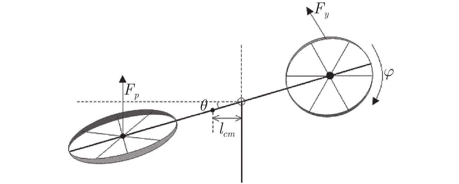
图 1 二自由度无人直升机简化图
Fig. 1 Simplified diagram of two degree of freedom unmanned helicopteropter

图 2 第I组参数下不受噪声污染时的数值结果
Fig. 2 Numerical results without noise pollution under parameters group I
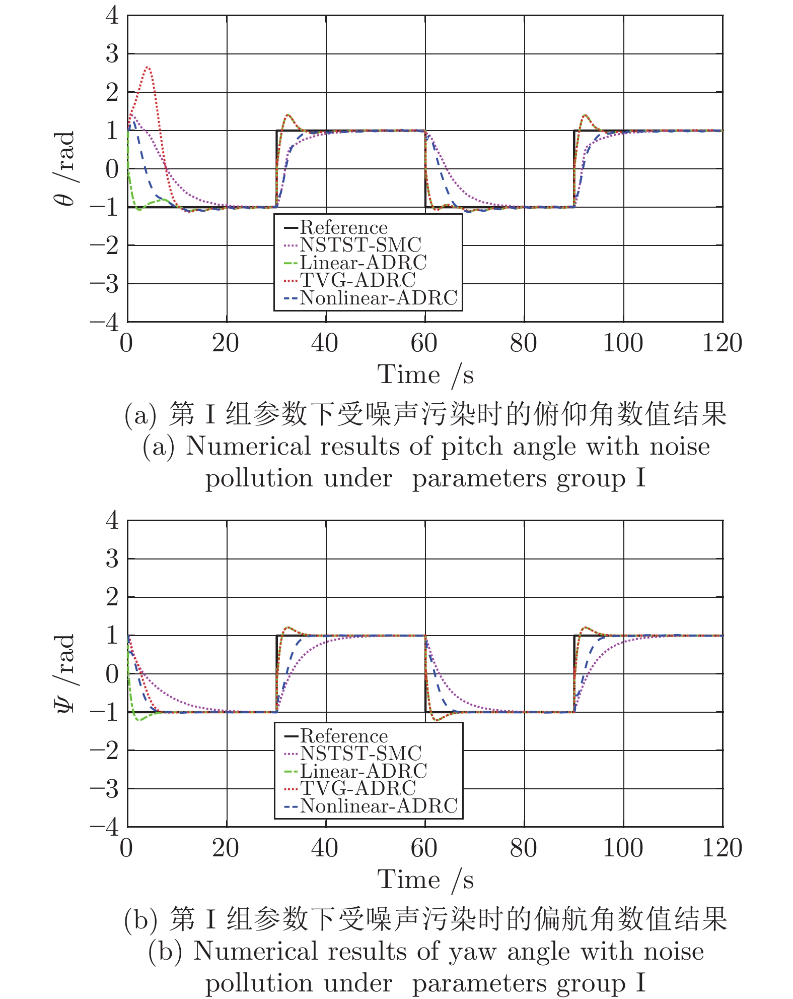
图 3 第I组参数下受噪声污染时的数值结果
Fig. 3 Numerical results with noise pollution under parameters group I
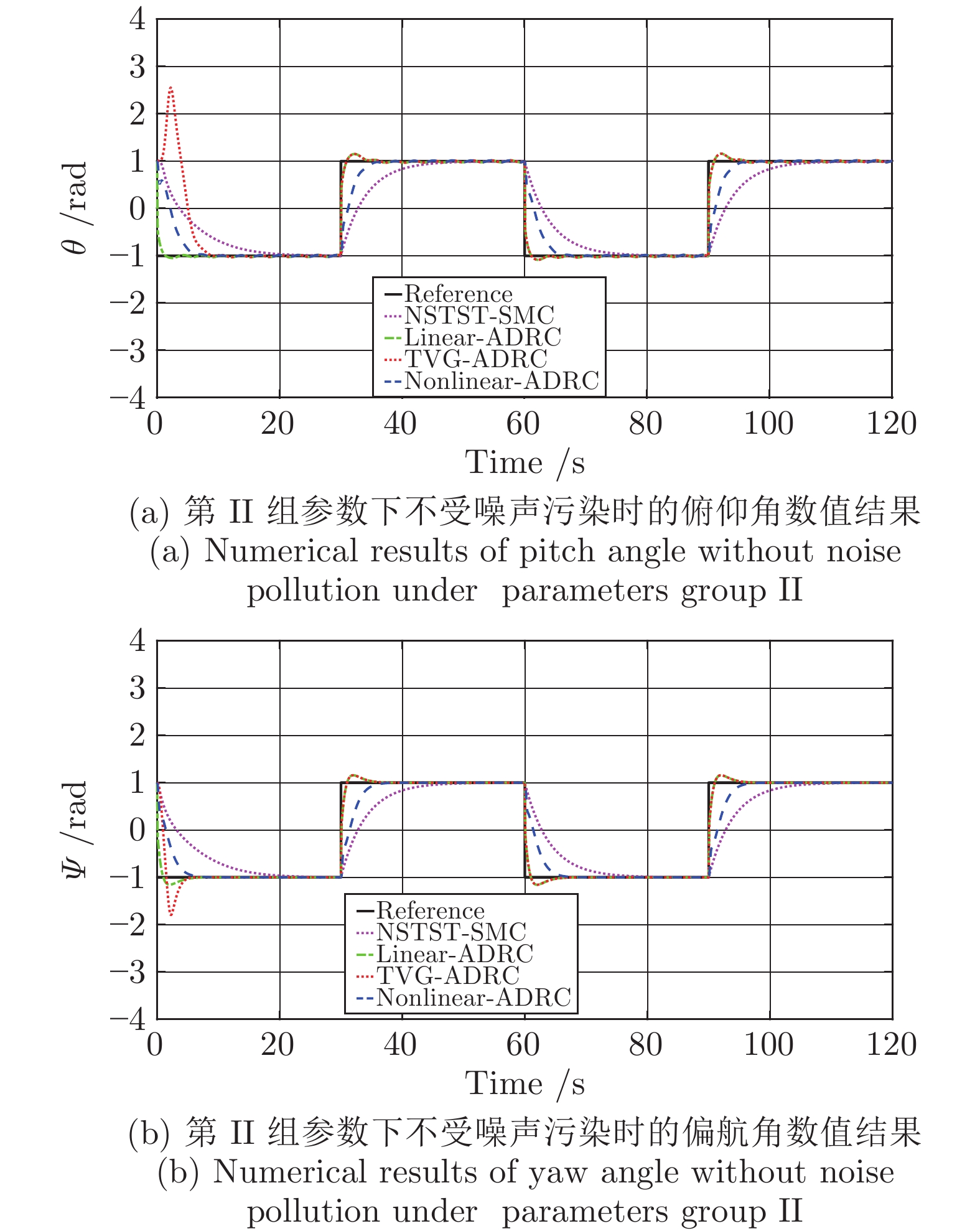
图 4 第II组参数下不受噪声污染时的数值结果
Fig. 4 Numerical results without noise pollution under parameters group II
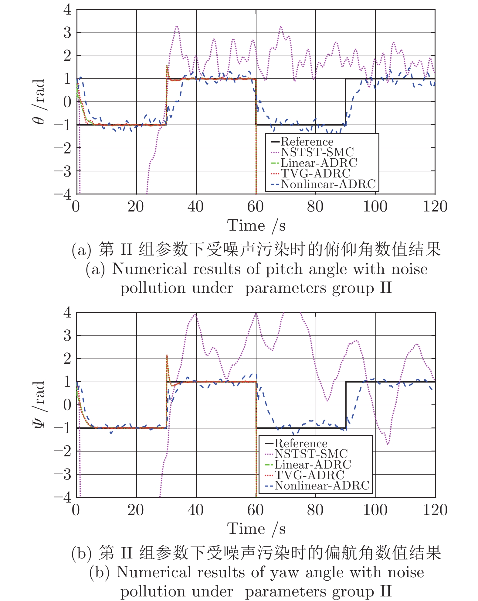
图 5 第II组参数下受噪声污染时的数值结果
Fig. 5 Numerical results with noise pollution under parameters group II

图 6 第III组参数下不受噪声污染时的数值结果
Fig. 6 Numerical results without noise pollution under parameters group III
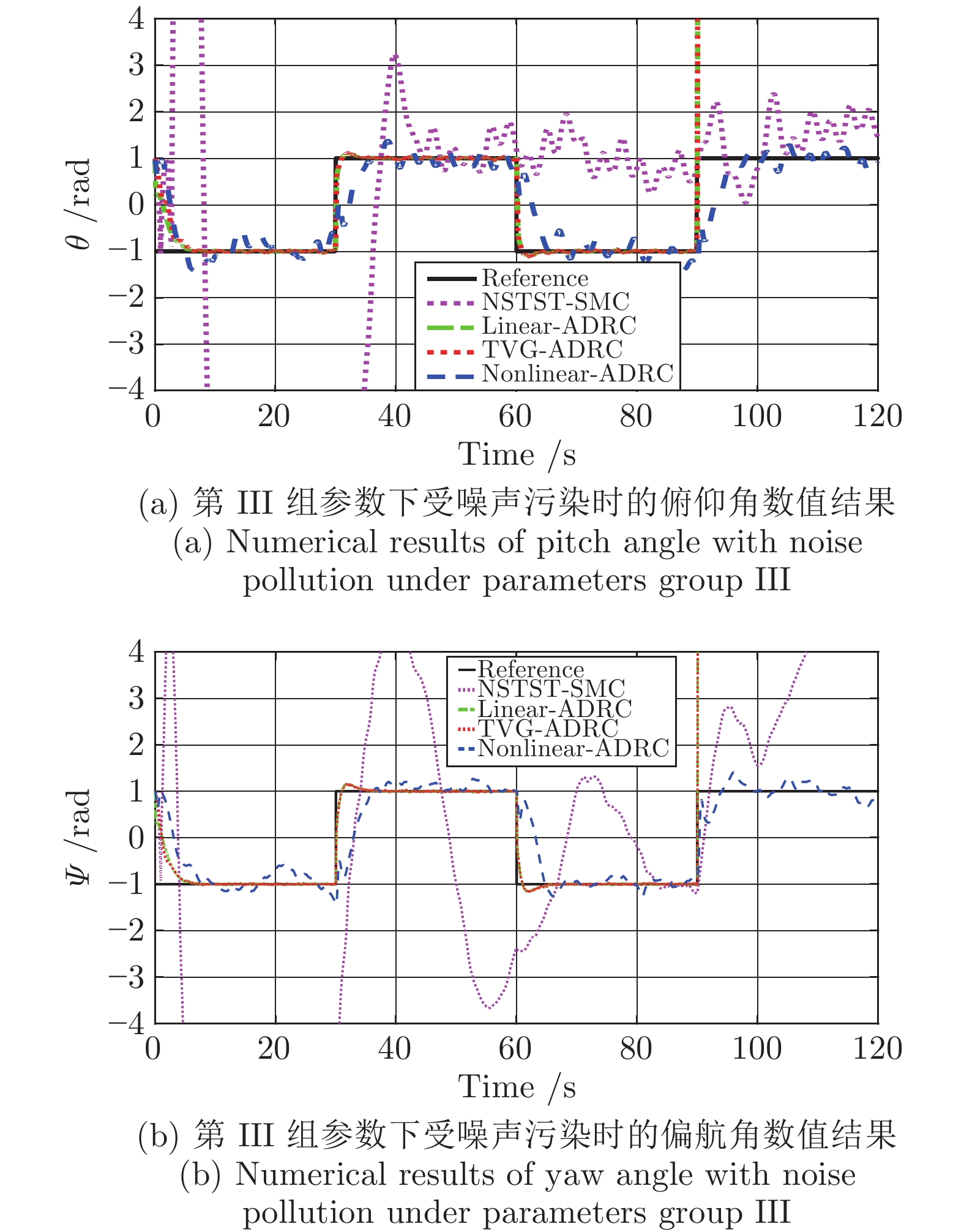
图 7 第III组参数下受噪声污染时的数值结果
Fig. 7 Numerical results with noise pollution under parameters group III
表 1 三组系统参数
Table 1 Three sets of system parameters
参数 I II III $\tau_{pp}\;({\rm{ {\rm{Nm/V} } } })$ 0.204 2.04 20.4 $\tau_{py}\;({\rm{Nm/V} })$ 0.0068 0.068 0.68 $\tau_{yy}\;({\rm{Nm/V} })$ 0.072 0.72 7.2 $\tau_{yp}\;({\rm{Nm/V} })$ 0.0219 0.219 2.19 $D_{p}\;(N/V)$ 0.8 8 80 $D_{y}\;(N/V)$ 0.318 3.18 31.8 $I_{p}\;({\rm{kg} }\cdot {\rm{m} }^{3})$ 0.0384 0.384 3.84 $I_{y}\;({\rm{kg} }\cdot {\rm{m} }^{3})$ 0.0432 0.432 4.32 $m \;({\rm{kg} })$ 1.3872 13.872 138.72 $l \;({\rm{m} })$ 0.186 1.86 18.6 $g\; ({\rm{m/s} }^{-2})$ 9.81 9.81 9.81  下载: 导出CSV
-
[1] Gao W N, Huang M Z, Jiang Z P, Chai T Y. Sampled-data-based adaptive optimal output-feedback control of a 2-degree-of-freedom helicopter. IET Control Theory & Applications, 2016, 10(12): 1440−1447 [2] Yu Z Q, Qu Y H, Zhang Y M. Safe control of trailing UAV in close formation flight against actuator fault and wake vortex effect. Aerospace Science and Technology, 2018, 77: 189−205 doi: 10.1016/j.ast.2018.01.028 [3] 王宁, 王永. 基于模糊不确定观测器的四旋翼飞行器自适应动态面轨迹跟踪控制. 自动化学报, 2018, 44(4): 685−695Wang Ning, Wang Yong. Fuzzy uncertainty observer based adaptive dynamic surface control for trajectory tracking of a quadrotor. Acta Automatica Sinica, 2018, 44(4): 685−695 [4] Song Z K, Sun K B. Adaptive compensation control for attitude adjustment of quad-rotor unmanned aerial vehicle. ISA Transactions, 2017, 69: 242−255 doi: 10.1016/j.isatra.2017.04.003 [5] SaiCharanSagar A, Vaitheeswaran S M, Shendge P D. Uncertainity estimation based approach to attitude control of fixed wing UAV. IFAC-PapersOnLine, 2016, 49(1): 278−283 doi: 10.1016/j.ifacol.2016.03.066 [6] Derafa L, El Hadri A, Fridman L. External perturbation estimation based on super-twisting algorithm for attitude control of UAVs. IFAC Proceedings Volumes, 2012, 45(13): 746−752 doi: 10.3182/20120620-3-DK-2025.00067 [7] Humaidi A J, Hasan A F. Particle swarm optimization–based adaptive super-twisting sliding mode control design for 2-degree-of-freedom helicopter. Measurement and Control, 2019, 52(9−10): 1403−1419 doi: 10.1177/0020294019866863 [8] Zhong Y J, Zhang Y M, Zhang W, Zuo J Y, Zhan H. Robust actuator fault detection and diagnosis for a quadrotor UAV with external disturbances. IEEE Access, 2018, 6: 48169−48180 doi: 10.1109/ACCESS.2018.2867574 [9] Muñoz F, González-Hernández I, Salazar S, Espinoza E S, Lozano R. Second order sliding mode controllers for altitude control of a quadrotor UAS: Real-time implementation in outdoor environments. Neurocomputing, 2017, 233: 61−71 doi: 10.1016/j.neucom.2016.08.111 [10] Guzey H M, Dierks T, Jagannathan S, Acar L. Modified consensus-based output feedback control of quadrotor UAV formations using neural networks. Journal of Intelligent & Robotic Systems, 2019, 94(1): 283−300 [11] Xin Y, Qin Z C, Sun J Q. Input-output tracking control of a 2-DOF laboratory helicopter with improved algebraic differential estimation. Mechanical Systems and Signal Processing, 2019, 116: 843−857 doi: 10.1016/j.ymssp.2018.07.027 [12] Ouyang Y C, Dong L, Xue L, Sun C Y. Adaptive control based on neural networks for an uncertain 2-DOF helicopter system with input deadzone and output constraints. IEEE/CAA Journal of Automatica Sinica, 2019, 6(3): 807−815 doi: 10.1109/JAS.2019.1911495 [13] Boukadida W, Benamor A, Messaoud H, Siarry H. Multi-objective design of optimal higher order sliding mode control for robust tracking of 2-DoF helicopter system based on metaheuristics. Aerospace Science and Technology, 2019, 91: 442−455 doi: 10.1016/j.ast.2019.05.037 [14] Sadala S P, Patre B M. A new continuous sliding mode control approach with actuator saturation for control of 2-DOF helicopter system. ISA Transactions, 2018, 74: 165−174 doi: 10.1016/j.isatra.2018.01.027 [15] Han J Q. From PID to active disturbance rejection control. IEEE Transactions on Industrial Electronics, 2009, 56(3): 900−906 doi: 10.1109/TIE.2008.2011621 [16] Dong L L, Zheng Q, Gao Z Q. On control system design for the conventional mode of operation of vibrational gyroscopes. IEEE Sensors Journal, 2008, 8(11): 1871−1878 doi: 10.1109/JSEN.2008.2006451 [17] Sun L, Li D H, Lee K Y. Enhanced decentralized PI control for fluidized bed combustor via advanced disturbance observer. Control Engineering Practice, 2015, 42: 128−139 doi: 10.1016/j.conengprac.2015.05.014 [18] Song K, Hao T Y, Xie H. Disturbance rejection control of air-fuel ratio with transport-delay in engines. Control Engineering Practice, 2018, 79: 36−49 doi: 10.1016/j.conengprac.2018.06.009 [19] 康莹, 李东海, 老大中. 航天器姿态的自抗扰控制与滑模控制的性能比较. 控制理论与应用, 2013, 30(12): 1623−1629 doi: 10.7641/CTA.2013.30993Kang Ying, Li Dong-Hai, Lao Da-Zhong. Performance comparison of active disturbance rejection control and sliding mode control in spacecraft attitude control. Control Theory & Applications, 2013, 30(12): 1623−1629 doi: 10.7641/CTA.2013.30993 [20] Ma Z Y, Zhu X P, Zhou Z. On-ground lateral direction control for an unswept flying-wing UAV. The Aeronautical Journal, 2019, 123(1261): 416−432 doi: 10.1017/aer.2018.167 [21] Zhang S C, Xue X Y, Chen C, Sun Z, Sun T. Development of a low-cost quadrotor UAV based on ADRC for agricultural remote sensing. International Journal of Agricultural and Biological Engineering, 2019, 12(4): 82−87 doi: 10.25165/j.ijabe.20191204.4641 [22] Yu B, Kim S, Suk J. Robust control based on ADRC and DOBC for small-scale helicopter. IFAC-PapersOnLine, 2019, 52(12): 140−145 doi: 10.1016/j.ifacol.2019.11.183 [23] Freidovich L B, Khalil H K. Performance recovery of feedback-linearization-based designs. IEEE Transactions on Automatic Control, 2008, 53(10): 2324−2334 doi: 10.1109/TAC.2008.2006821 [24] 陈增强, 孙明玮, 杨瑞光. 线性自抗扰控制器的稳定性研究. 自动化学报, 2013, 39(5): 574−580Chen Zeng-Qiang, Sun Ming-Wei, Yang Rui-Guang. On the stability of linear active disturbance rejection control. Acta Automatica Sinica, 2013, 39(5): 574−580 [25] Xue W C, Huang Y. Performance analysis of active disturbance rejection tracking control for a class of uncertain LTI systems. ISA Transactions, 2015, 58: 133−154 doi: 10.1016/j.isatra.2015.05.001 [26] Pu Z Q, Yuan R Y, Yi J Q, Tan X M. A class of adaptive extended state observers for nonlinear disturbed systems. IEEE Transactions on Industrial Electronics, 2015, 62(9): 5858−5869 doi: 10.1109/TIE.2015.2448060 [27] Shao S, Gao Z. On the conditions of exponential stability in active disturbance rejection control based on singular perturbation analysis. International Journal of Control, 2017, 90(10): 2085−2097 doi: 10.1080/00207179.2016.1236217 [28] Jiang T T, Huang C D, Guo L. Control of uncertain nonlinear systems based on observers and estimators. Automatica, 2015, 59: 35−47 doi: 10.1016/j.automatica.2015.06.012 [29] 金辉宇, 刘丽丽, 兰维瑶. 二阶系统线性自抗扰控制的稳定性条件. 自动化学报, 2018, 44(9): 1725−1728Jin Hui-Yu, Liu Li-Li, Lan Wei-Yao. On stability condition of linear active disturbance rejection control for second-order systems. Acta Automatica Sinica, 2018, 44(9): 1725−1728 [30] Guo B Z, Zhao Z L. Active Disturbance Rejection Control for Nonlinear Systems: An Introduction. New Jersey: John Wiley & Sons, 2016. [31] Fliess M, Levine J, Martin P, Rouchon P. A Lie-Backlund approach to equivalence and flatness of nonlinear systems. IEEE Transactions on Automatic Control, 1999, 44(5): 922−937 doi: 10.1109/9.763209 [32] She J H, Fang M X, Ohyama Y, Hashimoto H, Wu M. Improving disturbance-rejection performance based on an equivalent-input-disturbance approach. IEEE Transactions on Industrial Electronics, 2008, 55(1): 380−389 doi: 10.1109/TIE.2007.905976 [33] Zhong Q C, Kuperman A, Stobart R K. Design of UDE-based controllers from their two-degree-of-freedom nature. International Journal of Robust and Nonlinear Control, 2011, 21(17): 1994−2008 doi: 10.1002/rnc.1674 [34] Chen W H, Yang J, Guo L, Li S H. Disturbance-observer-based control and related methods: An overview. IEEE Transactions on Industrial Electronics, 2016, 63(2): 1083−1095 doi: 10.1109/TIE.2015.2478397 [35] 李杰, 齐晓慧, 夏元清, 高志强. 线性/非线性自抗扰切换控制方法研究. 自动化学报, 2016, 42(2): 202−212Li Jie, Qi Xiao-Hui, Xia Yuan-Qing, Gao Zhi-Qiang. On linear/nonlinear active disturbance rejection switching control. Acta Automatica Sinica, 2016, 42(2): 202−212 [36] 李向阳, 哀薇, 田森平. 惯性串联系统的自抗扰控制. 自动化学报, 2018, 44(3): 562−568Li Xiang-Yang, Ai Wei, Tian Sen-Ping. Active disturbance rejection control of cascade inertia systems. Acta Automatica Sinica, 2018, 44(3): 562−568 [37] Li S H, Yang J, Chen W H, Chen X S. Disturbance Observer-Based Control: Methods and Applications. Boca Raton: CRC Press, 2014. [38] Bai W Y, Chen S, Huang Y, Guo B Z, Wu Z H. Observers and observability for uncertain nonlinear systems: A necessary and sufficient condition. International Journal of Robust and Nonlinear Control, 2019, 29(10): 2960−2977 doi: 10.1002/rnc.4531 [39] Guo B Z, Wu Z H, Zhou H C. Active disturbance rejection control approach to output-feedback stabilization of a class of uncertain nonlinear systems subject to stochastic disturbance. IEEE Transactions on Automatic Control, 2016, 61(6): 1613−1618 doi: 10.1109/TAC.2015.2471815 [40] Zhao Z L, Guo B Z. A nonlinear extended state observer based on fractional power functions. Automatica, 2017, 81: 286−296 doi: 10.1016/j.automatica.2017.03.002 [41] Bhat S P, Bernstein D S. Geometric homogeneity with applications to finite-time stability. Mathematics of Control, Signals and Systems, 2005, 17(2): 101−127 doi: 10.1007/s00498-005-0151-x [42] Zhao Z L, Jiang Z P. Finite-time output feedback stabilization of lower-triangular nonlinear systems. Automatica, 2018, 96: 259−269 doi: 10.1016/j.automatica.2018.07.003 [43] Zhao Z L, Guo B Z. Active disturbance rejection control approach to stabilization of lower triangular systems with uncertainty. International Journal of Robust and Nonlinear Control, 2016, 26(11): 2314−2337 doi: 10.1002/rnc.3414 [44] Xue W C, Bai W Y, Yang S, Song K, Huang Y, Xie H. ADRC with adaptive extended state observer and its application to air-fuel ratio control in gasoline engines. IEEE Transactions on Industrial Electronics, 2015, 62(9): 5847−5857 doi: 10.1109/TIE.2015.2435004 -

 下载:
下载:

计量
- 文章访问数: 1654
- HTML全文浏览量: 484
- PDF下载量: 341
- 被引次数: 0
