

Dioxin Emission Concentration Soft Measurement Based on Multi-source Latent Feature Selective Ensemble Modeling for Municipal Solid Waste Incineration Process
-
摘要: 二噁英(Dioxin,DXN)是导致城市固废焚烧(Municipal solid waste incineration, MSWI)建厂存在“邻避现象”的主要原因之一. 工业现场多采用离线化验手段检测DXN浓度, 难以满足污染物减排控制的需求. 针对上述问题, 本文提出了基于潜在特征选择性集成(Selective ensemble, SEN)建模的DXN排放浓度软测量方法. 首先, 采用主元分析(Principal component analysis, PCA)分别提取依据工艺阶段子系统及全流程系统过程变量的潜在特征, 并依据预设贡献率阈值进行特征初选; 接着, 采用互信息(Mutual information, MI)度量初选特征与DXN间的相关性, 并自适应确定再选的上下限及阈值; 最后, 采用具有超参数自适应选择机制的最小二乘−支持向量机(Least squares — support vector machine, LS-SVM)算法建立多源特征的候选子模型, 基于分支定界(Branch and bound, BB)优化和预测误差信息熵加权算法进行集成子模型的优化选择和加权组合, 进而得到软测量模型. 基于某MSWI焚烧厂DXN检测数据仿真验证了所提方法的有效性.
-
关键词:
- 城市固废焚烧 /
- 二噁英 /
- 多源潜在特征 /
- 最小二乘−支持向量机 /
- 选择性集成建模
Abstract: One of the main reasons leading to “not in my backyard (NIMBY)” of municipal solid waste incineration (MSWI) plant construction is dioxin (DXN) emission from such process, which is a highly toxic substance to the ecological environment. In practical industrial process, the DXN emission concentration is detected by off-line. It is difficult to meet the requirements of optimal control. Aim at the above problem, a new DXN emission concentration soft measurement approach based on multi-source latent feature selective ensemble (SEN) modeling is proposed. Firstly, MSWI process is divided into different subsystems according to industrial processes. Principal component analysis (PCA) was used to extract their latent features. Primary selection of these features is made based on empirical pre-set threshold of contribution rate. Then, mutual information (MI) is used to measure the correlation between these primary selected features and DXN. The upper and lower limits and thresholds for re-selected feature are adaptively determined. Finally, based on the re-selected feature, the least squares-support vector machine (LS-SVM) algorithm with hyper-parameter adaptive selection mechanism is used to construct sub-models. A strategy based on branch and bound (BB) and prediction error information entropy weighting algorithm is used to select sub-model and calculate the weight coefficient. Thus, an SEN soft sensing model is obtained. The proposed method is verified by using DXN detection data of MSWI process in Beijing.1) 收稿日期 2019-03-27 录用日期 2019-06-27 Manuscript received March 27, 2019; accepted June 27, 2019 国家自然科学基金 (62073006, 62021003), 北京市自然科学基金 (4212032, 4192009), 科学技术部国家重点研发计划(2018YFC1900800-5), 矿冶过程自动控制技术国家(北京市)重点实验室(BGRIMM-KZSKL-2020-02)资助 Supported by National Natural Science Foundation of China (62073006, 62021003), Beijing Natural Science Foundation (4212032, 4192009), National Key Research and Development Program of the Ministry of Science and Technology (2018YFC1900800-5),2) and Beijing Key Laboratory of Process Automation in Mining and Metallurgy (BGRIMM-KZSKL-2020-02) 本文责任编委 刘艳军 Recommended by Associate Editor LIU Yan-Jun 1. 北京工业大学信息学部 北京 100124 2. 计算智能与智能系统北京市重点实验室 北京 100124 1. Faculty of Information Technology, Beijing University of Technology, Beijing 100124 2. Beijing Key Laboratory of Computational Intelligence and Intelligent System, Beijing 100124 -
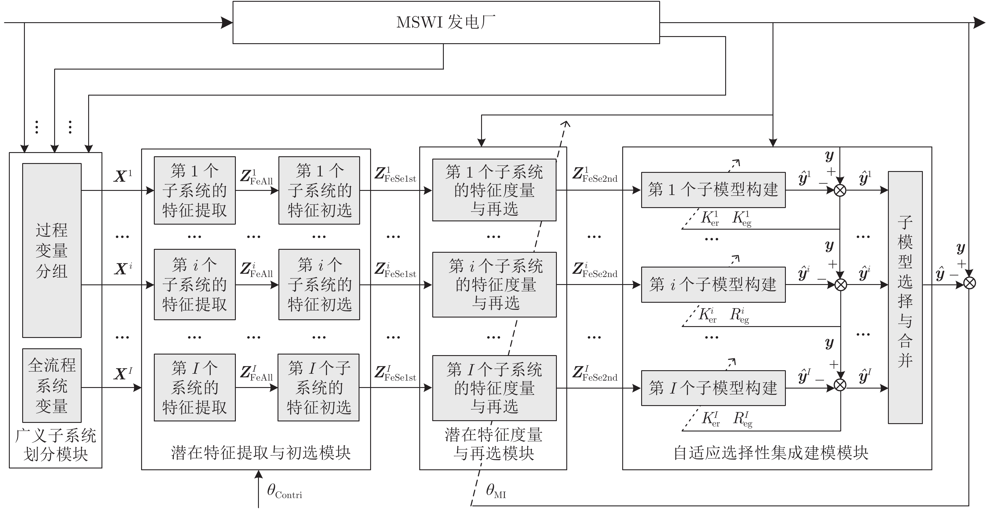
图 2 基于潜在特征SEN建模的DXN排放浓度软测量策略
Fig. 2 Soft sensing strategy of DXN emission concentration based on latent feature SEN modeling
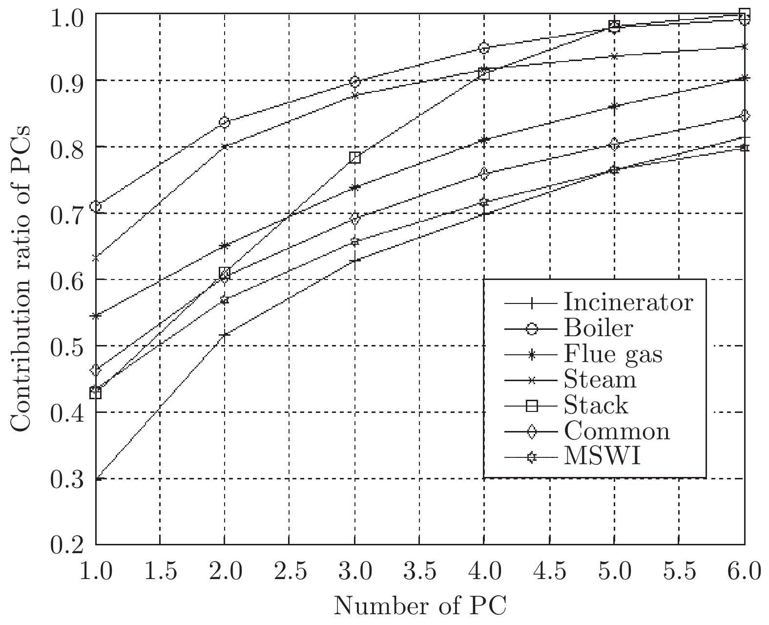
图 3 不同功能子系统的前6个PC的累积贡献率
Fig. 3 Cumulative contribution rate of the first six PCs of different functional subsystems
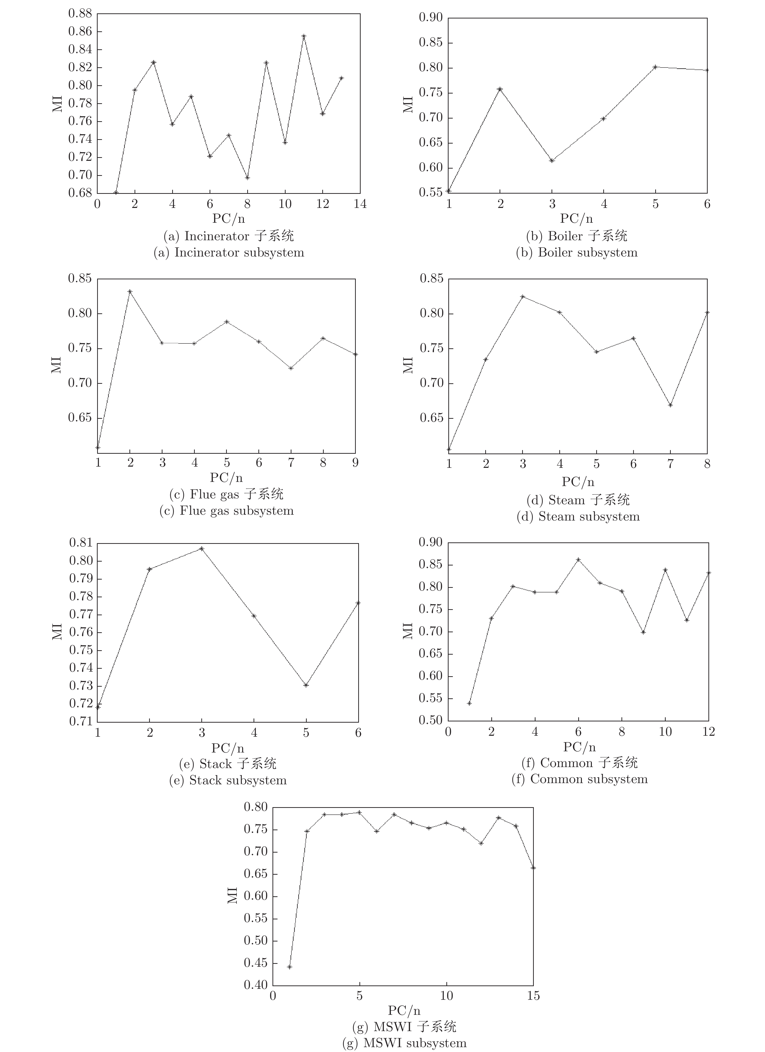
图 4 全部子系统及MSWI全流程系统的初选潜在特征与DXN间的MI值
Fig. 4 MI value between DXN and primary potential characteristics of all subsystems and MSWI whole process systems

图 5 子模型超参数自适应寻优的第1次和第2次的曲线
Fig. 5 Curves of the 1st and 2nd curves for adaptive hyperparametric optimization of submodels
表 1 本文中的公式符号及其说明汇总表
Table 1 Summary of formula symbols and their explanations in this paper
符号 含义 符号 含义 ${ {{\boldsymbol{y}}} }$ DXN 排放浓度软测量模型的真值 ${\boldsymbol{\hat y} }$ DXN排放浓度软测量模型的预测输出 $N$ 建模样本数量 $M$ 输入过程变量数量 ${ {{\boldsymbol{X}}} }$ MSWI 全流程系统的输入数据 ${\boldsymbol{X} }_{}^i$ 第$i$个子系统的输入数据 ${ {{\boldsymbol{I}} - 1} }$ MSWI 全流程系统划分子系统个数 $M_{}^i$ 第$i$个子系统包含的过程变量个数 ${ {{\boldsymbol{Z}}} }_{ {\rm{FeAll} } }^i$ 第$i$个子系统的过程变量采用PCA提取的全部潜在特征 $M_{{\rm{FeAll}}}^i$ 第$i$个子系统的过程变量采用PCA提取的全部潜在特征的数量 ${ {{\boldsymbol{Z}}} }_{ {\rm{FeSe1st} } }^i$ 第$i$个子系统的初选潜在特征 ${\theta _{{\rm{Contri}}}}$ 对全部潜在特征进行初选的设定阈值 $M_{{\rm{FeSe1st}}}^i$ 第$i$个子系统初选潜在特征的数量 $M_{{\rm{FeSe2nd}}}^i$ 第$i$个子系统再选潜在特征的数量 ${ {{\boldsymbol{Z}}} }_{ {\rm{FeSe2nd} } }^i$ 第$i$个子系统的再选潜在特征 ${\theta _{{\rm{MI}}}}$ 再选潜在特征的选择阈值${\theta _{{\rm{MI}}}}$ ($K_{{\rm{er}}}^i$, $R_{{\rm{eg}}}^i$) 第$i$个子模型的核参数和正则化参数 , 即超参数对 $i$ 第$i$个子模型的预测输出 ${ {{\boldsymbol{t}}} }_{m_{ {\rm{FeAll} } }^i}^i$ 第$i$个子系统的第$m_{ {\rm{FeAll} } }^i$个主元的得分向量 ${ {{\boldsymbol{p}}} }_{m_{ {\rm{FeAll} } }^i}^ii$ 第$i$个子系统的第$m_{ {\rm{FeAll} } }^i$个主元的载荷向量 ${ {{\boldsymbol{T}}} }_{}^i$ 第$i$个子系统的得分矩阵 ${\boldsymbol{P}}^i $ 第$i$个子系统的载荷矩阵 $\lambda _{m_{{\rm{FeAll}}}^i}^i$ 第$i$个子系统的第$m_{ {\rm{FeAll} } }^i$个载荷向量${\boldsymbol{p} }_{m_{ {\rm{FeAll} } }^i}^i$相对应的特征值 $\theta _{m_{{\rm{FeAll}}}^i}^i$ 第$i$个子系统的第$m_{ {\rm{FeAll} } }^i$个潜在特征的贡献率 $\xi _{m_{{\rm{FeAll}}}^i}^i$ 第$i$个子系统的第$m_{ {\rm{FeAll} } }^i$个潜在特征是否被选中的标记值 $\xi _{{\rm{MI}}}^{m_{{\rm{FeSelst}}}^i}$ 第$i$个子系统的初选潜在特征${\boldsymbol{z} }_{m_{ {\rm{FeSelst} } }^i}^i$与DXN排放浓度间的MI值 $\theta _{{\rm{Contri}}}^{{\rm{Uplimit}}}$ 潜在特征再选阈值的上限值 $\theta _{{\rm{Contri}}}^{{\rm{Downlimit}}}$ 潜在特征再选阈值的下限值 $\theta _{{\rm{Contri}}}^{{\rm{Step}}}$ 潜在特征再选阈值的固定步长 $\beta _{m_{{\rm{FeSe1st}}}^i}^i$ 第$i$个子系统的第$m_{ {\rm{FeSe1st} } }^i$个初选潜在特征是否被选中的标记值 ${ { {{\boldsymbol{w}}} }^i}$ 第$i$个子模型的权重系数 ${b^i}$ 第$i$个子模型的偏置系数 ${{\bf{\beta }}^i}$ 第$i$个子模型的拉格朗日算子向量 ${{\bf{\zeta }}^i}$ 第$i$个子模型的预测误差向量 $M_{{\rm{para}}}^{}$ 候选超参数矩阵 $\{ K_{{\rm{er}}}^i,R_{{\rm{eg}}}^i\} $ 第$i$个子模型在$M_{{\rm{para}}}^{}$中自适应选择的超参数对 $K$ 候选核参数数量 $R$ 候选惩罚参数数量 $J = K \times R$ 超参数矩阵中的超参数对的数量 $\begin{array}{l}\{ {(K_{{\rm{er}}}^{{\rm{initial}}})^i}, {(R_{{\rm{eg}}}^{{\rm{initial}}})^i}\}\end{array}$ 第$i$个子模型在采用网格搜索策略在矩阵$M_{{\rm{para}}}^{}$中初选的超参数对 ${({ {{\boldsymbol{K}}} }_{ {\rm{er} } }^{ {\rm{vector} } })^i}$ 依据初选超参数对计算的新候选核参数向量 ${({ {{\boldsymbol{R}}} }_{ {\rm{eg} } }^{ {\rm{vector} } })^i}$ 依据初选超参数对计算的新候选惩罚参数向量 ${N_{{\rm{ker}}}}$ 新候选核参数的数量 ${N_{{\rm{reg}}}}$ 新候选惩罚参数的数量 $k_{{\rm{supara}}}^{{\rm{down}}}$,$k_{{\rm{supara}}}^{{\rm{up}}}$ 确定超参数向量的收缩和扩放因子 ${f^i}( \cdot )$ 第$i$个子模型 ${f^{{i_{{\rm{sel}}}}}}( \cdot )$ 第${i_{ {\rm{sel} } } }$个集成子模型 $w_{{i_{{\rm{sel}}}}}^{}$ 第${i_{ {\rm{sel} } } }$个集成子模型的加权系数 ${\hat y_{{i_{{\rm{sel}}}}}}$ 第${i_{ {\rm{sel} } } }$个集成子模型的预测值 $K_{{\rm{er}}}^{{i_{{\rm{sel}}}}}$,$R_{{\rm{eg}}}^{{i_{{\rm{sel}}}}}$ 第${i_{ {\rm{sel} } } }$个集成子模型的超参数 ${(\hat y_{{i_{{\rm{sel}}}}}^{})_n}$ 第$n$个样本基于第${i_{ {\rm{sel} } } }$个集成子模型的预测值 ${(e_{{i_{{\rm{sel}}}}}^{})_n}$ 第$n$个样本基于第${i_{ {\rm{sel} } } }$个集成子模型的相对预测误差 $E_{{i_{{\rm{sel}}}}}^{}$ 第${i_{ {\rm{sel} } } }$个集成子模型的预测误差信息熵  下载: 导出CSV
表 2 初选潜在特征的数量及其贡献率
Table 2 Number of the primary selected latent feature and their contribution ratio
子系统代号 Incinerator Boiler Flue gas Steam Stack Common MSWI 特征编号 1 29.90 70.99 54.57 63.34 42.91 46.33 43.58 2 21.75 12.66 10.42 16.56 18.06 14.10 13.40 3 11.14 6.058 8.901 7.691 17.30 8.653 8.761 4 6.952 5.014 7.146 3.906 12.65 6.798 5.921 5 6.635 3.036 5.041 2.030 7.211 4.483 4.822 6 5.075 1.356 4.269 1.533 1.854 4.221 3.246 7 3.792 — 3.237 1.184 — 3.501 3.071 8 3.208 — 2.584 1.007 — 2.842 2.919 9 2.784 — 1.190 — — 2.116 2.444 10 1.846 — — — — 1.494 2.138 11 1.514 — — — — 1.256 1.911 12 1.283 — — — — 1.164 1.731 13 1.129 — — — — — 1.481 14 — — — — — — 1.344 15 — — — — — — 1.068 初选潜在特征数量 13 6 9 5 6 12 15 原始过程变量数量 79 14 19 53 6 115 286
下载: 导出CSV
表 3 全部子系统及MSWI全流程系统初选潜在特征MI值的极值统计表
Table 3 Extremum statistical table of potential characteristic MI values for primary selection latent feature of all Subsystems and MSWI whole process system
子系统 最大值集合 最小值集合 MI 值 贡献率 (%) PC 编号 MI 值 贡献率 (%) PC 编号 Incinerator 0.8559 1.514 11 0.6814 29.90 1 Boiler 0.8019 3.036 5 0.5527 70.99 1 Flue gas 0.8316 10.42 2 0.6084 54.57 1 Steam 0.8249 7.691 3 0.6059 63.34 1 Stack 0.8067 17.30 3 0.7182 42.91 1 Common 0.8613 4.221 6 0.5400 46.33 1 MSWI 0.7882 4.822 5 0.4429 43.58 1
下载: 导出CSV
表 4 再选潜在特征数量和MI值统计表
Table 4 Statistical table of re-selected latent feature's number and MI value
子系统 数量 MI值 Incinerator 5 0.7952 0.8267 0.8258 0.8559 0.8088 — Boiler 2 0.8019 0.7952 — — — — Flue gas 1 0.8316 — — — — — Steam 3 0.8249 0.8022 0.8019 — — — Stack 2 0.7952 0.8067 — — — — Common 6 0.8019 0.8613 0.8088 0.7904 0.8383 0.8316 MSWI 1 0.7882 — — — — —
下载: 导出CSV
表 5 不同建模方法统计结果
Table 5 Statistical results of different modeling methods
方法 过程变量数量 加权方法 RMSE 参数 (LV/PC) $( K_{ {\rm{er} } }^{},R_{ {\rm{eg} } }^{})$ 备注 文献 [22] 12 — 0.08869 ± 0.3000 (—) (—) 单模型, RWNN 文献 [24] 8 — 0.02695 (—) (21, 21) 单模型, SVM 文献 [37] 6 AWF 0.02306 (—) (0.1, 1; 400, 6400; 12800,
25600; 51200, 102400)SEN, 基于多核参数 PLS 286 — 0.01790 (13) (—) 单模型, MSWI系统 PCA-LS-SVM 286 — 0.01563 (18) (36240, 83904) 单模型, MSWI系统 集成建模 (EN) 286 PLS 0.01420 (5, 2, 1, 3, 2, 6, 1) (109, 109; 10000,
25.75; 5.950, 0.0595; 30.70, 2.080;
5.950, 0.5950; 1520800, 22816;
1362400, 158.5)
PCA-MI-LSSVM子模型, EN,
全部子模型AWF 0.01851 Entropy 0.01625 选择性集成建模(SEN) (本文方法) 286 (104) BB-AWF 0.01348 (5, 1, 2) (109, 109; 5.950, 0.0595; 5.950, 0.5950) PCA-MI-LSSVM子模型, SEN, Incinerator, Flue gas,
Stack共3个子模型BB-Entropy 0.01332
下载: 导出CSV
-
[1] 柴天佑. 复杂工业过程运行优化与反馈控制[J]. 自动化学报, 2013, 39(11): 1744-1757.Chai Tian-You. Operational optimization and feedback control for complex industrial processes. Acta Automatica Sinica, 2013, 39(11): 1744-1757 [2] Chai T Y, Ding J L, Yu G, Wang H. Integrated optimization for the automation systems of mineral processing. IEEE Transactions on Automation Science & Engineering, 2014, 11(4): 965-982. [3] Chai T Y, Qin S J, Wang H. Optimal operational control for complex industrial processes. Annu. Rev. Control, 2014, 38(1): 81-92. doi: 10.1016/j.arcontrol.2014.03.005 [4] Arafat H A, Jijakli K, Ahsan A. Environmental performance and energy recovery potential of five processes for municipal solid waste treatment. Journal of Cleaner Production, 2015, 105: 233-240. doi: 10.1016/j.jclepro.2013.11.071 [5] Yuanan H, Hefa C, Shu T. The growing importance of waste-to-energy (WTE) incineration in China's anthropogenic mercury emissions: Emission inventories and reduction strategies. Renewable and Sustainable Energy Reviews, 2018, 97: 119-137. doi: 10.1016/j.rser.2018.08.026 [6] Huang T, Zhou L, Liu L, Xia M. Ultrasound-enhanced electrokinetic remediation for removal of Zn, Pb, Cu and Cd in municipal solid waste incineration fly ashes. Waste Management, 2018, 75: 226-235. doi: 10.1016/j.wasman.2018.01.029 [7] Jones P H, Degerlache J, Marti E, Mischer G, Scherrer M C, Bontinck W J, Niessen H J. The global exposure of man to dioxins - a perspective on industrial-waste incineration. Chemosphere, 1993, 26: 1491-1497. doi: 10.1016/0045-6535(93)90216-R [8] Li X, Zhang C, Li Y, Zhi Q. The Status of Municipal Solid Waste Incineration (MSWI) in China and its Clean Development. Energy Procedia, 2016, 104: 498-503. doi: 10.1016/j.egypro.2016.12.084 [9] Phillips K, Longhurst P J, Wagland S T. Assessing the perception and reality of arguments against thermal waste treatment plants in terms of property prices. Waste Management. 2014, 34(1): 219-225. doi: 10.1016/j.wasman.2013.08.018 [10] Zhang H J, Ni Y W, Chen J P, Zhang Q. Influence of variation in the operating conditions on PCDD/F distribution in a full-scale MSW incinerator. Chemosphere, 2008, 70(4): 721-730. doi: 10.1016/j.chemosphere.2007.06.054 [11] Mukherjee A, Debnath B, Ghosh S K. A review on technologies of removal of dioxins and furans from incinerator flue gas. Procedia Environmental Sciences, 2016, 35: 528-540. doi: 10.1016/j.proenv.2016.07.037 [12] Stanmore B R. Modeling the formation of PCDD/F in solid waste incinerators. Chemosphere, 2002, 47: 565-773. doi: 10.1016/S0045-6535(02)00005-X [13] 乔俊飞, 郭子豪, 汤健. 面向城市固废焚烧过程的二噁英排放浓度检测方法综述. 自动化学报, 2020, 46(6): 1063−1089Qiao Jun-Fei, Guo Zi-Hao, Tang Jian. Dioxin emission concentration measurement approaches for municipal solid wastes incineration process: A survey. Acta Automatica Sinica, 2020, 46(6): 1063−1089 [14] Pandelova M, Lenoir D, Schramm K W. Correlation between PCDD/F, PCB and PCBz in coal/waste combustion Influence of various inhibitors. Chemosphere, 2006, 62: 1196-1205. doi: 10.1016/j.chemosphere.2005.07.068 [15] Gullett B K, Oudejans L, Tabor D, Touati A, Ryan S. Near-real-time combustion monitoring for PCDD/PCDF indicators by GC-REMPI-TOFMS. Environmental Engineering Science, 2012, 46: 923-928. [16] Wang W, Chai T Y, Yu W, Wang H, Su C Y. Modeling component concentrations of sodium aluminate solution via hammerstein recurrent neural networks. IEEE Transactions on Control Systems Technology, 2012, 20(4): 971−982 [17] Tang J, Chai T Y, Yu W, Zhao L J. Modeling load parameters of ball mill in grinding process based on selective ensemble multisensor information. IEEE Transactions on Automation Science & Engineering, 2013, 10(3): 726-740. [18] Li D C, Liu C W. Extending attribute information for small data set classication. IEEE Transactions on Knowledge and Data Engineering, 2010, 24(3): 452-464 [19] 汤健, 乔俊飞, 柴天佑, 刘卓, 吴志伟. 基于虚拟样本生成技术的多组分机械信号建模. 自动化学报, 2018, 44(9): 1569-1590.Tang Jian, Qiao Jun-Fei, Chai Tian-You, Liu Zhuo, Wu Zhi-Wei. Modeling Multiple Components Mechanical Signals by Means of Virtual Sample Generation Technique. Acta Automatica Sinica, 2018, 44(9): 1569-1590. [20] Chang N B, Huang S H. Statistical modelling for the prediction and control of PCDDs and PCDFs emissions from municipal solid waste incinerators. Waste Management & Research, 1995, 13: 379-400. [21] Chang N B, Chen W C. Prediction of PCDDs/PCDFs emissions from municipal incinerators by genetic programming and neural network modeling. Waste Management & Research, 2000, 18(4): 41-351. [22] Bunsan S, Chen W Y, Chen H W, Chuang Y H, Grisdanurak N. Modeling the dioxin emission of a municipal solid waste incinerator using neural networks. Chemosphere, 2013, 92: 258-264. doi: 10.1016/j.chemosphere.2013.01.083 [23] Gomes T A F, Prud êncio R B C, Soares C, Rossi A L D, Carvalho A. Combining meta-learning and search techniques to select parameters for support vector machines. Neurocomputing, 2012, 75(1): 3-13. doi: 10.1016/j.neucom.2011.07.005 [24] 肖晓东, 卢加伟, 海景, 等. 垃圾焚烧烟气中二噁英类浓度的支持向量回归预测. 可再生能源, 2017, 35(8): 1107-1114Xiao Xiao-Dong, Lu Jia-Wei, Hai Jing. Prediction of dioxin emissions in flue gas from waste incineration based on support vector regression. Renewable Energy Resources, 2017, 35(8): 1107-1114. [25] Tang J, Chai T Y, Yu W, Zhao L J. Feature extraction and selection based on vibration spectrum with application to estimate the load parameters of ball mill in grinding process. Control Engineering Practice, 2012, 20(10): 991-1004. doi: 10.1016/j.conengprac.2012.03.020 [26] Soares C. A hybrid meta-learning architecture for multi-objective optimization of SVM parameters. Neurocomputing, 2014, 143(143): 27-43. [27] Yu G, Chai T Y, Luo X C. Multiobjective production planning optimization using hybrid evolutionary algorithms for mineral processing. IEEE Transact. Evolut. Comput. 2011, 15(4): 487-514. doi: 10.1109/TEVC.2010.2073472 [28] Yin S, Yin J. Tuning kernel parameters for SVM based on expected square distance ratio. Information Sciences, 2016, 370-371: 92-102. doi: 10.1016/j.ins.2016.07.047 [29] Tang J, liu Z, Zhang J, Wu Z W, Chai T Y, Yu W. Kernel latent feature adaptive extraction and selection method for multi-component non-stationary signal of industrial mechanical device, Neurocomputing, 2016, 216(C): 296-309. [30] 汤健, 田福庆, 贾美英. 基于频谱数据驱动的旋转机械设备负荷软测量. 北京: 国防工业出版社, 2015.Tang Jian, Tian Fu-Qing, Jia Mei-Ying. Soft Measurement of Rotating Machinery Equipment Load Based on Spectrum Data Drive. Beijing: National Defense Industry Press, 2015. [31] Brown G, Wyatt J, Harris R, Yao X. Diversity creation methods: a survey and categorisation. Information Fusion, 2005, 6: 5-20 doi: 10.1016/j.inffus.2004.04.004 [32] Tang J, Chai T Y, Yu W, Liu Z, Zhou X J. A Comparative study that measures ball mill load parameters through different single-scale and multi-scale frequency spectra-based approaches, IEEE Transactions on Industrial Informatics. 2016, 12(6): 2008-2019. doi: 10.1109/TII.2016.2586419 [33] Zhou Z H, Wu J, Tang W, Ensembling neural networks: many could be better than all, Artificial Intelligence, 2002, 137(1-2): 239-263. doi: 10.1016/S0004-3702(02)00190-X [34] Ma G, Wang Y, Wu L. Subspace ensemble learning via totally-corrective boosting for gait recognition. Neurocomputing, 2017, 224: 119-127. doi: 10.1016/j.neucom.2016.10.047 [35] Tang J, Qiao J, Wu Z W, et al. Vibration and acoustic frequency spectra for industrial process modeling using selective fusion multi-condition samples and multi-source features. Mechanical Systems and Signal Processing, 2018, 99: 142-168. doi: 10.1016/j.ymssp.2017.06.008 [36] Soares S, Antunes C H, Rui Ara újo. Comparison of a genetic algorithm and simulated annealing for automatic neural network ensemble development. Neurocomputing, 2013, 121(18): 498-511. [37] 汤健, 乔俊飞. 基于选择性集成核学习算法的固废焚烧过程二噁英排放浓度软测量, 化工学报, 2019, 70(2): 696−706Tang Jian, Qiao Jun-Fei. Dioxin emission concentration soft measuring approach of municipal solid waste incineration based on selective ensemble kernel learning algorithm, Journal of Chemical Industry and Engineering (China), 2019, 70(2): 696−706 [38] Tang J, Chai T, Liu Z, et al. Selective ensemble modeling based on nonlinear frequency spectral feature extraction for predicting load parameter in ball mills. Chinese Journal of Chemical Engineering, 2015, 23(12): 2020-2028. doi: 10.1016/j.cjche.2015.10.006 -

 下载:
下载:


计量
- 文章访问数: 1094
- HTML全文浏览量: 335
- PDF下载量: 164
- 被引次数: 0
