

Image Splicing Detection Based on Spatial Lighting Consistency Analysis Under Perspective Projection
-
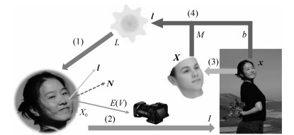
摘要: 将一个人的头像剪切并拼接到另一张照片中,是一种常见的图像篡改手段.如果将该合成照片用于敲诈勒索,会对社会带来严重危害.因此,用来检测图像篡改的图像取证技术具有重大意义.由于不同照片成像环境不同,拼接时很难做到不同人脸的光照绝对一致,因此可以通过光照是否一致检测篡改.以往光照估计方法基于平行投影的假设,利用照片投影光照进行光照一致性分析.实际上,相机针孔模型是透视投影,从而导致上述检测方法出现误差.针对这一问题,本文提出一种透视投影下物体空间光照估计算法,将各人脸姿态统一到相机坐标系下,估计各人脸相对于相机坐标系的空间光照,然后分析空间光照一致性.另外,根据人脸空间光照一致性约束可以优化出相机参数,并得到该参数下的等效焦距、人脸空间位置及重新透视投影的图像等空间信息.本文将空间光照的一致性和上述空间信息的合理性作为依据,对人脸图像进行拼接篡改检测.实验结果表明,相比于传统方法基于平行投影光照进行光照一致性分析,采用本文提出的方法得到的空间光照进行光照一致性分析具有更高的准确度,结合相关信息进行照片空间合理性分析的篡改检测方法具有更强的说服力.Abstract: Splicing a face image of a person into another photo is a common tempering way, and it is harmful once used for blackmail. Therefore, the image forensics for tampered image detection is of great significance. As different photos are taken in different environments with different cameras, it is very difficult to ensure the spliced faces have absolutely consistent light. Thus the illumination consistency can be an effective clue for tempering detection. Existing illumination consistency analysis based tempering detection methods perform the illumination estimation under the assumption of parallel projection. However, the results usually have huge but subtle errors because the camera pinhole model is perspective projection. To solve this problem, we propose a spatial lighting estimation method under perspective projection for the illumination consistency analysis. In addition, the spatial information analysis is combined to obtain more reasonable detection results. Specifically, the coordinate system of each face is firstly unified into the camera coordinate system and the spatial lighting of each face relative to the camera coordinate system is estimated. Then the camera parameters are optimized according to the consistency constraint of faces' spatial lighting and the spatial information including the equivalent focal length, face spatial position and re-perspective projection image under the camera parameters are calculated. Finally, the consistency of spatial lighting and the rationality of the spatial information are both taken as clues to detect face image splicing forgery. The experimental results show that compared with previous methods, the spatial lighting estimation method has higher accuracy, and the spatial information analysis method has stronger persuasion.
-
Key words:
- Image forensics /
- lighting estimation /
- spatial lighting /
- perspective projection /
- splicing detection
-
在工业生产和社会生活中, 存在着大量的复杂系统, 如非线性耦合机械系统[1]、超临界机组[2]等. 这些复杂系统线性化时通常包含了不可控模态, 给其控制器设计与分析带来了挑战. 在过去十几年里, 这类称之为高阶非线性系统的自适应控制问题吸引了很多研究者的关注. Lin等在文献[3-4]中提出了一种新的构造性设计框架−增加幂次积分法, 有效解决了高阶非线性系统的镇定与实际跟踪问题. 借助于这一方法, 文献[5-19]研究了不同条件下高阶不确定非线性系统的自适应控制问题, 取得了一系列研究成果. 值得指出的是, 上述绝大多数研究结果都要求系统的幂次信息完全已知. 然而, 在一些实际应用中, 由于控制系统本身与周围环境存在着各种不确定因素, 使得系统的幂次信息可能无法精确获取. 因此, 进一步探讨具有未知幂次的高阶非线性系统的控制器设计是很有意义并值得研究的问题.
针对具有未知幂次的高阶非线性系统, 文献[20-21]采用改进的增加幂次积分法, 分别给出了状态反馈和输出反馈控制算法. 然而, 这些算法没有考虑系统函数的不确定性, 且需要假设系统的幂次上界信息已知. 文献[22]结合增加幂次积分技术和自适应控制方法, 解决了具有未知幂次和不确定参数的高阶非线性系统的自适应控制问题. 最近, 针对一类具有未知时变幂次的高阶非线性系统, 文献[23]利用障碍李雅普诺夫方法给出了满足全状态约束条件的自适应控制方案. 但文献[22-23]所提控制方案仍然要求系统幂次的上界已知. 为去除这一假设条件, 文献[24]采用增加幂次积分技术和逻辑切换方法, 设计了一种全局切换自适应镇定方案. 该方案的不足在于切换控制信号是非光滑的, 可能会引起抖振问题, 从而激发系统中的高频未建模动态. 为此, 文献[25]利用动态增益法, 提出了一种光滑自适应状态反馈控制器, 但这种控制器仅适用于相对阶为2的非线性系统.
基于以上讨论, 本文研究了一类具有未知幂次的高阶不确定非线性系统的自适应跟踪控制问题. 结合积分反推技术和障碍李雅普诺夫函数, 提出了一种新颖的自适应状态反馈控制策略. 本文所得到的控制策略具有如下优点: 1) 采用对数型障碍李雅普诺夫函数[26-27]解决了系统幂次未知与模型不确定带来的技术难题; 2) 所提出的自适应控制策略中没有包含虚拟控制律的导数信息, 避免了积分反推法中的“计算膨胀”问题; 3) 所设计控制器能够确保闭环系统的所有信号一致有界. 最后, 仿真结果验证了本文理论结果的有效性.
本文采用如下符号:
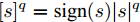
$ {\bf{R}} $ ,${\bf{R}}_{\geq{{0}}}$ ,${\bf{R}}_{ > {{0}}}$ 分别表示实数、非负实数和正实数集合.$ {{\bf{R}}}^n $ 表示$ n $ 维实向量集合.$ {\rm{sign}}(s) $ 表示变量$ s $ 的符号函数. 对任意正常数$ q $ , 定义$ [s]^q = {\rm{sign}}(s)|s|^q $ .${\bf{Q}}_{{\rm{odd}}}^{\ge 1}$ 表示分子和分母都是正奇整数的所有有理数的集合.1. 问题描述与预备知识
1.1 问题描述
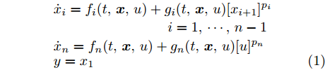
考虑如下高阶不确定非线性系统
$$ \begin{split} & \dot{x}_i = f_i(t,{\boldsymbol{x}},u)+g_i(t,{\boldsymbol{x}},u)[x_{i+1}]^{p_i}\\ &\qquad\qquad\qquad\;\;\;\;\quad i = 1,\cdots,n-1\\ &\dot{x}_n = f_n(t,{\boldsymbol{x}},u)+g_n(t,{\boldsymbol{x}},u)[u]^{p_n}\\& y = x_1 \end{split} $$ (1) 其中,
${\boldsymbol{x}} = [x_1,\cdots,x_n]^{\rm{T}}\in {{\bf{R}}}^n$ 是系统的状态向量, 初始值${\boldsymbol{x}}(0) = [x_1(0),\cdots,x_n(0)]^{\rm{T}}$ ,$\bar{{\boldsymbol{x}}}_i = [x_1,\cdots,x_i]^{\rm{T}}\in {{\bf{R}}}^i$ ,$i = 1,\cdots,n$ ;$ u \in {{\bf{R}}} $ 和$ y \in {{\bf{R}}} $ 分别是控制输入和系统输出;$ p_i\in {\bf{Q}}_{{\rm{odd}}}^{\ge 1} $ ,$i = 1,\cdots,n$ 是系统(1)的未知幂次. 系统函数$ f_i, g_i:{{\bf{R}}}_{\ge0}\times {{\bf{R}}}^n\times {{\bf{R}}}\rightarrow {{\bf{R}}} $ ,$i = 1,\cdots,n$ 在$ t $ 上分段连续, 且关于$ {\boldsymbol{x}} $ 和$ u $ 满足局部Lipschitz条件. 本文的控制目标是设计自适应控制器$ u $ , 使得系统输出$ y $ 跟踪期望轨迹$ y_r $ , 同时确保闭环系统的所有信号皆有界.注 1. 不同于文献[20-25]中的研究结果, 本文中系统幂次无需满足
$ p_1\ge p_2\ge \cdots\ge p_n $ .假设 1. 存在未知的连续函数
$\bar{f}_{il}(\bar{{\boldsymbol{x}}}_i) : {{\bf{R}}}^{i}\rightarrow {{\bf{R}}}_{\geq0}$ ,$ \underline{g}_i(\bar{{\boldsymbol{x}}}_i): {{\bf{R}}}^{i}\rightarrow {{\bf{R}}}_{>0} $ 和$ \bar{g}_i(\bar{{\boldsymbol{x}}}_i): {{\bf{R}}}^{i}\rightarrow {{\bf{R}}}_{>0} $ , 满足$$ |f_i(t,{\boldsymbol{x}},u)|\le \sum\limits_{l = 1}^{j_i}|x_{i+1}|^{q_{il}}\bar{f}_{il}(\bar{{\boldsymbol{x}}}_i) $$ (2) $$ 0<\underline{g}_i(\bar{{\boldsymbol{x}}}_i)\le g_i(t,{\boldsymbol{x}},u)\le \bar{g}_i(\bar{{\boldsymbol{x}}}_i) $$ (3) 其中,
$i = 1,\cdots,n$ ,$l = 1,\cdots,j_i$ ,$ j_i $ 为有限正整数,$ q_{il} $ 为满足$ 0\le q_{i1}<q_{i2}<\cdots<q_{ij_i}<p_i $ 的正常数.注 2. 假设1表明了本文所提控制算法无需知晓系统函数
$ g_i(t,{\boldsymbol{x}},u) $ ,$ f_i(t,{\boldsymbol{x}},u) $ 及相应的界函数$ \underline{g}_i(\bar{{\boldsymbol{x}}}_{i}) $ ,$ \bar{g}_i(\bar{{\boldsymbol{x}}}_{i}) $ ,$ \bar{f}_{il}(\bar{{\boldsymbol{x}}}_i) $ 的解析表达式.假设 2. 期望轨迹
$ y_r $ 为连续可微函数, 且存在未知正常数$ B_r $ , 满足$$ |y_r(t)|+|\dot{y}_r(t)|\le B_r,t\ge 0 $$ (4) 1.2 预备知识
引理 1[28]. 考虑初值问题
$$ \dot{\boldsymbol{\eta}}_r(t) = h_r(t,{\boldsymbol{\eta}}_r),\; {\boldsymbol{\eta}}_r(0) = {\boldsymbol{\eta}}^0_r\in \Xi_r $$ (5) 其中,
$h_r:{{\bf{R}}}_{\ge0}\times \Xi_r\rightarrow {{\bf{R}}}^{{N}}$ 在$ t $ 上分段连续, 且关于$ {\boldsymbol{\eta}}_r $ 满足局部Lipschitz条件,$\Xi_r\subset {{\bf{R}}}^{{N}}$ 为非空开子集.$ {\boldsymbol{\eta}}_r(t) $ 是初值问题(5)在最大存在区间$ [0,t'_f) $ 上的解,$ t'_f<+\infty $ . 设$ \Xi'_r $ 是$ \Xi_r $ 的紧子集, 则存在$t_s\in [0,t'_f)$ , 使得$ {\boldsymbol{\eta}}_r(t_s)\not\in\Xi'_r $ .引理 2[29]. 对任意
$ a\in {{\bf{R}}} $ ,$ b \in {{\bf{R}}} $ ,$ m\in {{\bf{R}}}_{>0} $ ,$ n\in {{\bf{R}}}_{>0} $ 和函数$ \rho(a,b)>0 $ , 下列不等式成立$$\begin{split} |a|^m|b|^n \le\;& \frac{m}{m+n}\rho(a,b)|a|^{m+n}\;+\\&\frac{n}{m+n}\rho(a,b)^{-\tfrac{m}{n}}|b|^{m+n} \end{split}$$ (6) 引理 3[29-30]. 对任意
$ p\ge 1 $ ,$ a\in {{\bf{R}}} $ ,$ b \in {{\bf{R}}} $ , 下列不等式成立$$ \|a|^{p}-|b|^{p}|\le |[a]^{p}-[b]^{p}| \hspace{37pt} $$ (7) $$ \begin{split} \,|[a]^{p}-[b]^{p}|\le\; &c_{p}|a-b|\times\\ &(|a-b|^{{p}-1}+|b|^{{p}-1}) \end{split} $$ (8) $$ |a|^{p}+|b|^{p}\le(|a|+|b|)^{p} \hspace{45pt}$$ (9) 其中,
$ c_{p} = 2^{p-2}+2 $ .引理 4[31]. 对任意
$ \delta\in {{\bf{R}}}_{>0} $ 和$ \xi \in {{\bf{R}}} $ , 下列不等式成立$$ 0\le |\xi|-\frac{\xi^2}{\sqrt{\xi^2+\delta^2}}<\delta $$ (10) 引理 5[32]. 对满足
$ 0\le d<c $ 的$ c\in {{\bf{R}}} $ 和$ d\in {{\bf{R}}} $ , 下列不等式成立$$ \log\frac{c}{c-d} \le \frac{d}{c-d} $$ (11) 2. 自适应跟踪控制策略
本节设计了一种基于障碍李雅普诺夫函数的自适应跟踪控制器, 并给出了闭环系统的稳定性证明.
2.1 自适应控制器设计
定义如下误差坐标变换
$$ z_1 = x_1-y_r $$ (12) $$ z_i = x_i-\alpha_{i-1},\;i = 2,\cdots,n $$ (13) 其中,
$ \alpha_{i-1} $ 是第$ i-1 $ 步的虚拟控制律.步骤
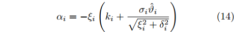
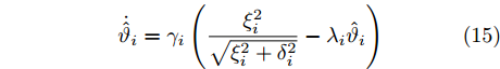
$ {\boldsymbol{i}} $ ${\boldsymbol{(i = 1,\cdots,n-1)}}$ . 选取正常数$ \mu_i $ 满足$ \mu_i>|z_i(0)| $ , 设计第$ i $ 步虚拟控制律和自适应律为$$ \alpha_i = -\xi_i\left(k_i+\frac{\sigma_i\hat{\vartheta}_i}{\sqrt{\xi_i^2+\delta_i^2}}\right) $$ (14) $$ \dot{\hat{\vartheta}}_i = \gamma_i\left(\frac{\xi_i^2}{\sqrt{\xi_i^2+\delta_i^2}}-\lambda_i\hat{\vartheta}_i\right) $$ (15) 其中,
$\xi_i = \dfrac{z_i}{\mu_i^2-z_i^{2}}$ ,$ \hat{\vartheta}_i $ 是$ \vartheta_i $ 的估计值,$ \hat{\vartheta}_i(0)\ge 0 $ ,$ k_i $ ,$ \sigma_i $ ,$ \gamma_i $ 和$ \lambda_i $ 为正常数.步骤 n. 选取正常数
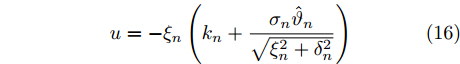
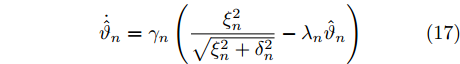
$ \mu_n $ 满足$ \mu_n>|z_n(0)| $ , 设计实际控制律和自适应律为$$ u = -\xi_n\left(k_n+\frac{\sigma_n\hat{\vartheta}_n}{\sqrt{\xi_n^2+\delta_n^2}}\right) $$ (16) $$ \dot{\hat{\vartheta}}_n = \gamma_n\left(\frac{\xi_n^2}{\sqrt{\xi_n^2+\delta_n^2}}-\lambda_n\hat{\vartheta}_n\right) $$ (17) 其中,
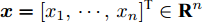
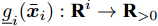
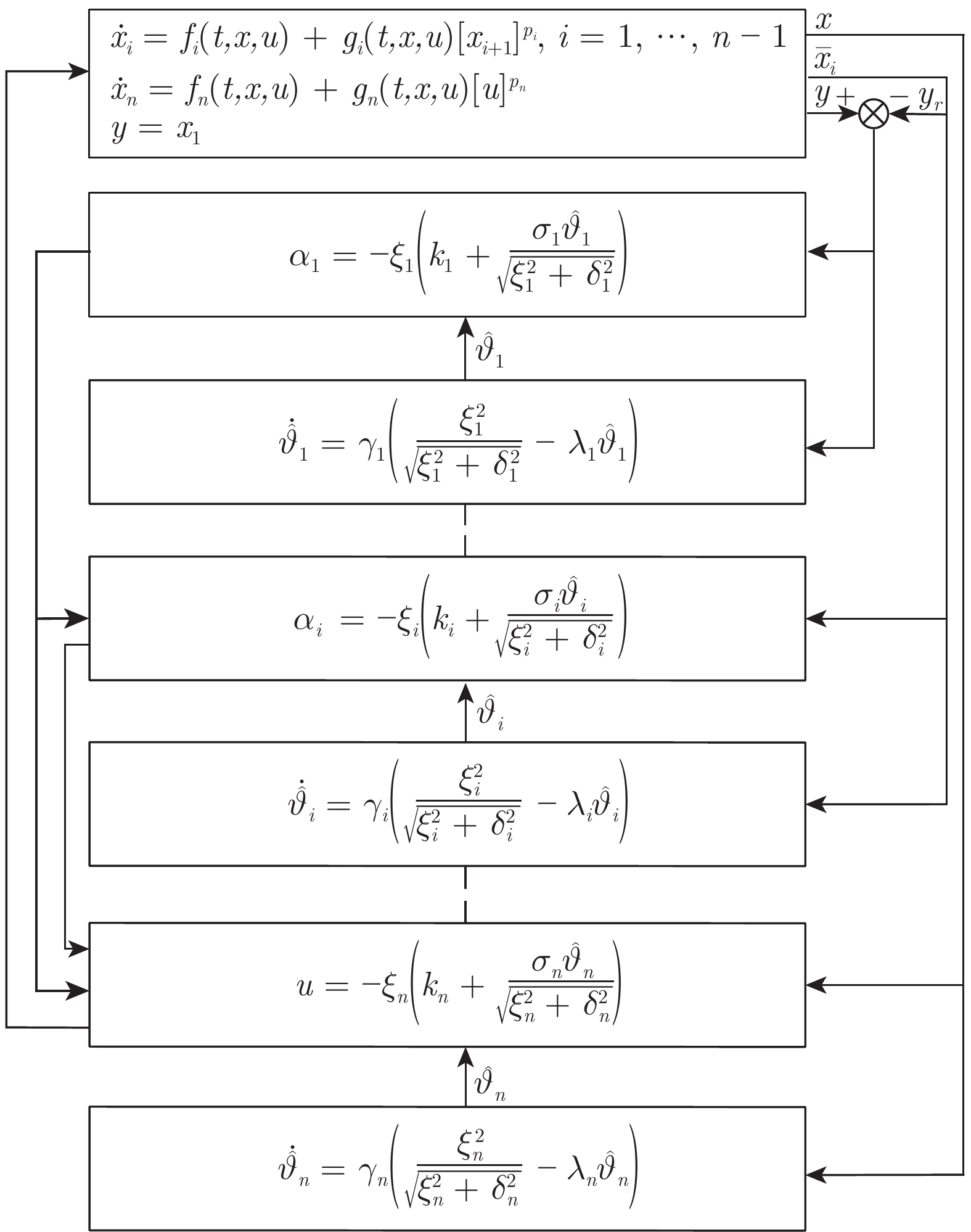
$\xi_n = \dfrac{z_n}{\mu_n^2-z_n^{2}}$ ,$ \hat{\vartheta}_n $ 是$ \vartheta_n $ 的估计值且满足,$\hat{\vartheta}_n(0)\ge 0$ ,$ k_n $ ,$ \sigma_n $ ,$ \gamma_n $ 和$ \lambda_n $ 为正常数.上述自适应控制器的设计过程如图1所示.
注 3. 如式(14) ~ (17)所示, 本文提出的自适应反推控制策略不依赖于系统幂次
$ p_i $ 及其上界信息, 且无需知晓系统函数$ f_i(t,{\boldsymbol{x}},u) $ ,$ g_i(t,{\boldsymbol{x}},u) $ 及相应的界函数$ \bar{f}_{il}(\bar{{\boldsymbol{x}}}_i) $ ,$ \underline{g}_i(\bar{{\boldsymbol{x}}}_{i}) $ ,$ \bar{g}_i(\bar{{\boldsymbol{x}}}_{i}) $ 的解析表达式. 同时, 该控制策略未包含虚拟控制律$ \alpha_i $ 的导数, 消除了积分反推法中“计算膨胀”问题.2.2 稳定性分析
在给出闭环系统的稳定性分析之前, 先引入如下命题.
命题 1. 对式(14) ~ (17)的
$\hat{\vartheta}_1,\cdots,\hat{\vartheta}_n, \alpha_1,\cdots, \alpha_{n-1}$ 和$ u $ , 下列陈述成立i)
$ \hat{\vartheta}_i(t)\ge 0 $ ,$i = 1,\cdots,n$ .ii)
$\xi_i[\alpha_i]^{p_i} = -|\xi_i||\alpha_i|^{p_i} \le 0, \xi_n [u]^{p_n} = -|\xi_n| |u|^{p_n}$ ,$i = 1,\cdots,n-1$ .证明. i) 由于
$\dfrac{\xi_i^2}{\sqrt{\xi_i^2+\delta_i^2}}\ge 0$ 和$ \hat{\vartheta}_i(0)\ge 0 $ , 根据式(15)和式(17), 可直接推出$ \hat{\vartheta}_i(t)\ge 0 $ ,$i = 1,\cdots,n$ .ii) 根据式(14)和式(16),
$ \alpha_i $ ,$i = 1,\cdots,n-1$ 和$ u $ 改写为$$ \alpha_i = \xi_i\phi_i,i = 1,\cdots,n-1 $$ (18) $$ u = \xi_n\phi_n\hspace{74pt} $$ (19) 其中,
$$ \phi_i = -k_i-\frac{\sigma_i\hat{\vartheta}_i}{\sqrt{\xi_i^2+\delta_i^2}},\;\;i = 1,\cdots,n $$ (20) 从而, 有
$$ \begin{split} \xi_i[\alpha_i]^{p_i} =&\; \xi_i|\alpha_i|^{p_i}{\rm{sign}}(\xi_i\phi_i)\\& \quad i = 1,\cdots,n-1\end{split} $$ (21) $$ \xi_n [u]^{p_n} = \xi_n |u|^{p_n}{\rm{sign}}(\xi_n\phi_n) $$ (22) 另外, 由于
$ \hat{\vartheta}_i(t)\ge 0 $ ,$i = 1,\cdots,n$ , 从式(20)易知$ \phi_i\le 0 $ ,$i = 1,\cdots,n$ , 进而可得${\rm{sign}}(\xi_i\phi_i) = -{\rm{sign}}(\xi_i)$ ,$i = 1,\cdots,n$ . 故$$ \begin{split} \xi_i[\alpha_i]^{p_i} =&\; -|\xi_i||\alpha_i|^{p_i}\le 0\\ & i = 1,\cdots,n-1 \end{split}$$ (23) $$ \xi_n [u]^{p_n} = -|\xi_n| |u|^{p_n}\le 0 $$ (24) □
本文主要结论可总结为如下定理.
定理 1. 对满足假设1和假设2的高阶不确定非线性系统(1), 在任意初始条件
$ {\boldsymbol{x}}(0) $ 下, 控制器(16)以及自适应律(15)和(17)保证了闭环系统的所有信号一致有界, 并且输出跟踪误差可以收敛到残差为任意小的残差集.证明. 本证明共分为3部分. 首先, 证明由系统(1), 控制器(16), 自适应律(15)和(17)组成的闭环系统在最大存在区间
$ [0,t_f) $ 上存在唯一解${\pmb\eta}(t) = [z_1(t),\cdots,z_n(t),\hat{\vartheta}_1(t),\cdots,\hat{\vartheta}_n(t)]^{\rm{T}}$ . 然后, 采用反证法证明$ t_f = +\infty $ . 最后, 实现本文控制目标.Part 1. 根据式(14)和式(16), 虚拟控制律
$\alpha_1,\cdots, \alpha_{n-1}$ , 实际控制律$ u $ 以及系统状态$x_1,\cdots,x_n$ 可写为$$ \alpha_i = \check{\alpha}_i(z_i,\hat{\vartheta}_i),i = 1,\cdots,n-1 $$ (25) $$ u = \check{\alpha}_n(z_n,\hat{\vartheta}_n) $$ (26) $$ x_1 = z_1+y_r= \check{x}_1(t,z_1) $$ (27) $$ \begin{split} x_i =\; & z_i+\check{\alpha}_{i-1}(t,z_{i-1},\hat{\vartheta}_{i-1})=\\ & \check{x}_i(t,z_{i-1},z_i,\;\hat{\vartheta}_{i-1}),i = 2,\cdots,n \end{split} $$ (28) 因此, 由式(1)和式(14)
$ \sim $ (17)组成的闭环系统可改写为$$ \begin{split} \dot{z}_1 =\;& f_1(t,\check{{\boldsymbol{x}}},\check{\alpha}_n)+g_1(t,\check{{\boldsymbol{x}}},\check{\alpha}_n)[\check{x}_2]^{p_1}-\dot{y}_r=\\ &\varphi_1(t,z_1,\cdots,z_n,\hat{\vartheta}_1,\cdots,\hat{\vartheta}_n) \end{split} $$ (29) $$ \begin{split} \dot{z}_i = \;& f_i(t,\check{{\boldsymbol{x}}},\check{\alpha}_n)+g_i(t,\check{{\boldsymbol{x}}},\check{\alpha}_n)[\check{x}_{i+1}]^{p_i}\;-\\ &\frac{\partial \check{\alpha}_{i-1}}{\partial t}-\frac{\partial \check{\alpha}_{i-1}}{\partial z_{i-1}}\varphi_{i-1}-\gamma_{i-1}\frac{\partial \check{\alpha}_{i-1}}{\partial \hat{\vartheta}_{i-1}}\;\times\\ &\left(\frac{\xi_{i-1}^2}{\sqrt{\xi_{i-1}^2+\delta_{i-1}^2}}-\lambda_{i-1}\hat{\vartheta}_{i-1}\right)=\\ & \varphi_i(t,z_1,\cdots,z_n,\hat{\vartheta}_1,\cdots,\hat{\vartheta}_n),\\ &\qquad\qquad\qquad\qquad\;\; i = 2,\cdots,n-1 \end{split}$$ (30) $$ \begin{split} \dot{z}_n =\; &f_n(t,\check{{\boldsymbol{x}}},\check{\alpha}_n)+g_n(t,\check{{\boldsymbol{x}}},\check{\alpha}_n)[\check{\alpha}_n]^{p_n}-\\ &\frac{\partial \check{\alpha}_{n-1}}{\partial t}-\frac{\partial \check{\alpha}_{n-1}}{\partial z_{n-1}}\varphi_{n-1}-\gamma_{n-1}\frac{\partial \check{\alpha}_{n-1}}{\partial \hat{\vartheta}_{n-1}}\times\\ &\left(\frac{\xi_{n-1}^2}{\sqrt{\xi_{n-1}^2+\delta_{n-1}^2}}-\lambda_{n-1}\hat{\vartheta}_{n-1}\right)=\\& \varphi_n(t,z_1,\cdots,z_n,\hat{\vartheta}_1,\cdots,\hat{\vartheta}_n) \end{split}$$ (31) $$ \begin{split} \dot{\hat{\vartheta}}_i =\;& \gamma_i\Big(\frac{\xi_i^2}{\sqrt{\xi_i^2+\delta_i^2}}-\lambda_i\hat{\vartheta}_i\Big)=\\ & \varphi_{n+i}(t,z_i,\hat{\vartheta}_i),\;\;i = 1,\cdots,n \end{split} $$ (32) 其中,
$\check{{\boldsymbol{x}}} = [\check{x}_1,\cdots,\check{x}_n]^{\rm{T}}\in {{\bf{R}}}^n$ .定义开集
$$ \Xi = \underbrace{(-\mu_1,\mu_1)\times\cdots\times(-\mu_n,\mu_n)}_n\times {{\bf{R}}}^n $$ 由于
$\mu_i > |z_i(0)|$ ,$i = 1,\cdots,n$ , 可知${\boldsymbol{\eta}}(0) = [z_1(0), \cdots, z_n(0),\hat{\vartheta}_1(0),\cdots,\hat{\vartheta}_n(0)]^{\rm{T}}\in \Xi$ . 同时, 由于期望参考信号$ y_r $ 及其导数$ \dot{y}_r $ 有界, 函数$ f_i, g_i $ ,$i = 1,\cdots, n$ 在$ t $ 上分段连续, 且关于$ {\boldsymbol{x}} $ 和$ u $ 满足局部Lipschitz条件, 可推得$ \varphi_i:{{\bf{R}}}_{\ge0}\times \Xi\rightarrow {{\bf{R}}} $ 在$ t $ 上分段连续, 且关于$ {\boldsymbol{x}} $ 和$ u $ 满足局部Lipschitz条件. 根据微分方程解的存在唯一性定理[33], 对任意初始条件$ {\boldsymbol{\eta}}(0) $ , 闭环系统(29) ~ (32)在最大存在区间$ [0,t_f) $ 上存在唯一解${\boldsymbol{\eta}} = [z_1,\cdots,z_n,\hat{\vartheta}_1,\cdots,\hat{\vartheta}_n]^{\rm{T}}\in \Xi$ , 即, 对$\forall t\in [0,t_f)$ ,$ |z_i|<\mu_i $ ,$i = 1,\cdots,n$ .Part 2. 本部分采用反证法证明
$ t_f = +\infty $ . 为此, 不妨假设$ t_f<+\infty $ .考虑如下障碍李雅普诺夫函数[26]:
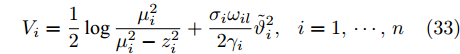
$$ V_i = \frac{1}{{2}}\log\frac{\mu_i^2}{\mu_i^2-z_i^{2}}+\frac{\sigma_i\omega_{il} }{2\gamma_i}\tilde{\vartheta}_i^2,\;\;i = 1,\cdots,n $$ (33) 其中,
$ \tilde{\vartheta}_i = \vartheta_i-\hat{\vartheta}_i $ ,$ \omega_{il} $ 是未知正常数.步骤
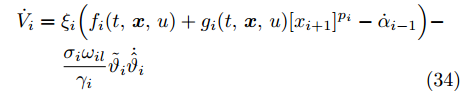
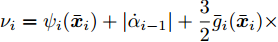
$ {\boldsymbol{i}} $ ${\boldsymbol{(i = 1,\cdots,n-1)}}$ .$ V_i $ 的导数为$$ \begin{split} \dot{V}_i = \;&\xi_i\Big(f_i(t,{\boldsymbol{x}},u)+g_i(t,{\boldsymbol{x}},u)[x_{i+1}]^{p_i}-\dot{\alpha}_{i-1}\Big)-\\ &\frac{\sigma_i\omega_{il} }{\gamma_i}\tilde{\vartheta}_i\dot{\hat{\vartheta}}_i \\[-10pt]\end{split}$$ (34) 其中,
$ \alpha_0 = y_r $ .根据假设1和引理2, 下列不等式成立
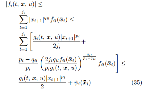
$$ \begin{split} &|f_i(t,{\boldsymbol{x}},u)|\le\\ &\qquad\sum\limits_{l = 1}^{j_i}|x_{i+1}|^{q_{il}}\bar{f}_{il}(\bar{{\boldsymbol{x}}}_i)\le\\ &\qquad\sum\limits_{l = 1}^{j_i}\Bigg[\frac{g_i(t,{\boldsymbol{x}},u)|x_{i+1}|^{p_i}}{2j_i}+\\ &\qquad\frac{p_i-q_{il}}{p_i}\left(\frac{2j_iq_{il}\bar{f}_{il}(\bar{{\boldsymbol{x}}}_i)}{p_ig_i(t,{\boldsymbol{x}},u)}\right)^{\frac{q_{il}}{p_i-q_{il}}}\bar{f}_{il}(\bar{{\boldsymbol{x}}}_i)\Bigg]\le\\ &\qquad\frac{g_i(t,{\boldsymbol{x}},u)|x_{i+1}|^{p_i}}{2}+\psi_i(\bar{{\boldsymbol{x}}}_i) \end{split} $$ (35) 其中,
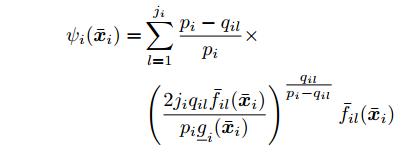
$$ \begin{split} \psi_i(\bar{{\boldsymbol{x}}}_i) =& \sum\limits_{l = 1}^{j_i}\frac{p_i-q_{il}}{p_i}\times\\ &\left(\frac{2j_iq_{il}\bar{f}_{il}(\bar{{\boldsymbol{x}}}_i)}{p_i\underline{g}_i(\bar{{\boldsymbol{x}}}_i)}\right)^{\tfrac{q_{il}}{p_i-q_{il}}}\bar{f}_{il}(\bar{{\boldsymbol{x}}}_i) \end{split}$$ 将式(35)代入式(34), 可得
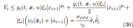
$$ \begin{split} \dot{V}_i\le\; &g_i(t,{\boldsymbol{x}},u)\xi_i [x_{i+1}]^{p_i}+\frac{g_i(t,{\boldsymbol{x}},u)|\xi_i|}{2}|x_{i+1}|^{p_i}+\\& |\xi_i|\Big(\psi_i(\bar{{\boldsymbol{x}}}_i)+|\dot{\alpha}_{i-1}|\Big)-\frac{\sigma_i\omega_{il} }{\gamma_i}\tilde{\vartheta}_i\dot{\hat{\vartheta}}_i \\[-10pt]\end{split}$$ (36) 根据命题1, 可得
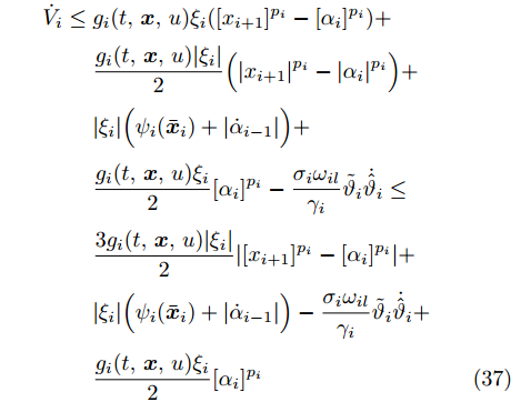
$$ \begin{split} \dot{V}_i\le \;&g_i(t,{\boldsymbol{x}},u)\xi_{i}([x_{i+1}]^{p_i}-[\alpha_{i}]^{p_i})+\\ &\frac{g_i(t,{\boldsymbol{x}},u)|\xi_i|}{2}\Big(|x_{i+1}|^{p_i}-|\alpha_{i}|^{p_i}\Big)+\\ &|\xi_i|\Big(\psi_i(\bar{{\boldsymbol{x}}}_i)+|\dot{\alpha}_{i-1}|\Big)+\\ &\frac{g_i(t,{\boldsymbol{x}},u)\xi_{i}}{2}[\alpha_i]^{p_i}-\frac{\sigma_i\omega_{il} }{\gamma_i}\tilde{\vartheta}_i\dot{\hat{\vartheta}}_i\le\\ &\frac{3g_i(t,{\boldsymbol{x}},u)|\xi_i|}{2}|[x_{i+1}]^{p_i}-[\alpha_{i}]^{p_i}|+\\ &|\xi_i|\Big(\psi_i(\bar{{\boldsymbol{x}}}_i)+|\dot{\alpha}_{i-1}|\Big)-\frac{\sigma_i\omega_{il} }{\gamma_i}\tilde{\vartheta}_i\dot{\hat{\vartheta}}_i+\\& \frac{g_i(t,{\boldsymbol{x}},u)\xi_{i}}{2}[\alpha_i]^{p_i} \end{split}$$ (37) 为了处理式(37)中的项
$ |\xi_i||[x_{i+1}]^{p_i}-[\alpha_{i}]^{p_i}| $ , 考虑以下两种情形.情形 1. 当
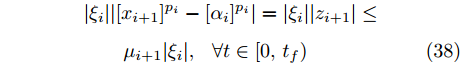
$ p_i = 1 $ 时. 由Part 1可得:$|z_{i+1}| < \mu_{i+1}$ ,$ \forall t\in [0,t_f) $ , 因而$$ \begin{split} &|\xi_i||[x_{i+1}]^{p_i}-[\alpha_{i}]^{p_i}|= |\xi_i||z_{i+1}|\le\\ &\qquad \mu_{i+1}|\xi_i|, \;\;\forall t\in [0,t_f) \end{split} $$ (38) 情形 2. 当
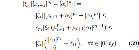
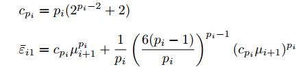
$ p_i>1 $ 时. 由引理2和引理3以及$|z_{i+1}| < \mu_{i+1}$ ,$ \forall t\in [0,t_f) $ , 可得$$\begin{split} &|\xi_i||[x_{i+1}]^{p_i}-[\alpha_{i}]^{p_i}|=\\ &\quad\; \; \; \; |\xi_i||[z_{i+1}+\alpha_{i}]^{p_i}-[\alpha_{i}]^{p_i}|\le\\ &\quad\; \; \; \; c_{p_i}|\xi_i|(\mu_{i+1}^{p_i}+\mu_{i+1}|\alpha_i|^{p_i-1})\le\\ &\quad\; \; \; \; |\xi_i|\Big(\frac{|\alpha_i|^{p_i}}{6}+\bar{\varepsilon}_{i1}\Big),\;\;\forall t\in [0,t_f) \end{split}$$ (39) 其中,
$$ \begin{split} &c_{p_i} = p_i(2^{p_i-2}+2)\\ &\bar{\varepsilon}_{i1} = c_{p_i}\mu_{i+1}^{p_i}+\frac{1}{p_i}\left(\frac{6(p_i-1)}{p_i}\right)^{p_i-1}(c_{p_i}\mu_{i+1})^{p_i} \end{split}$$ 综合情形1和情形2, 项
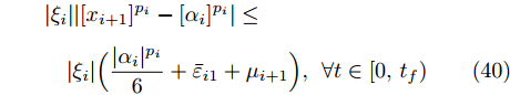
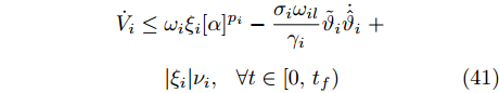
$ |\xi_i||[x_{i+1}]^{p_i}-[\alpha_{i}]^{p_i}| $ 放缩为$$ \begin{split} &|\xi_i||[x_{i+1}]^{p_i}-[\alpha_{i}]^{p_i}| \le\\ &\quad|\xi_i|\Big(\frac{|\alpha_i|^{p_i}}{6}+\bar{\varepsilon}_{i1}+\mu_{i+1}\Big),\;\forall t\in [0,t_f) \end{split} $$ (40) 将式(40)代入式(37)中, 并结合命题1, 易得
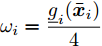
$$ \begin{split} \dot{V}_i\le\;&\omega_i\xi_{i}[\alpha]^{p_i}-\frac{\sigma_i\omega_{il} }{\gamma_i}\tilde{\vartheta}_i\dot{\hat{\vartheta}}_i\;+\\ &|\xi_i|\nu_i,\;\;\forall t\in [0,t_f) \end{split} $$ (41) 其中,
$\omega_i = \dfrac{\underline{g}_i(\bar{{\boldsymbol{x}}}_i)}{4}$ ,$\nu_i = \psi_i(\bar{{\boldsymbol{x}}}_i)+|\dot{\alpha}_{i-1}|+\dfrac{3}{2}\bar{g}_i(\bar{{\boldsymbol{x}}}_{i})\times (\bar{\varepsilon}_{i1}+ \mu_{i+1})$ .由Part 1可知, 对
$ \forall t\in [0,t_f) $ ,$ |z_j|<\mu_j $ ,$j = 1, \cdots, i$ . 同时, 依据假设1和假设2,$ y_r $ ,$ \dot{y}_r $ 有界, 且$ \bar{f}_{il} $ ,$ \underline{g}_i $ 和$ \bar{g}_i $ 为连续函数. 此外, 根据第$ i-1 $ 步设计, 可推知$x_1,\cdots,x_i$ ,$ \dot{\alpha}_{i-1} $ 有界,$ \forall t\in [0,t_f) $ . 因此, 运用极值定理, 对$ \forall t\in [0,t_f) $ , 有$$ 0< \omega_{il}\le \omega_i \, $$ (42) $$ 0\le \nu_i\le \nu_{im} $$ (43) 其中,
$ \omega_{il} $ 和$ \nu_{im} $ 为未知正常数.将式(42)和式(43)代入式(41)中, 有
$$ \begin{split} \dot{V}_i\le\;&\omega_{il}\xi_{i}[\alpha_i]^{p_i}-\frac{\sigma_i\omega_{il} }{\gamma_i}\tilde{\vartheta}_i\dot{\hat{\vartheta}}_i+\\ &\nu_{im}|\xi_i|,\;\;\forall t\in [0,t_f) \end{split} $$ (44) 通过式(14)和式(15), 并结合引理3, 可得
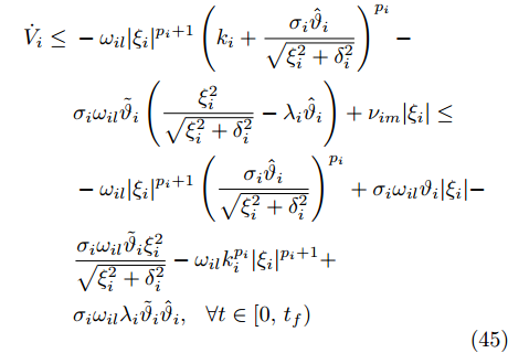
$$ \begin{split} \dot{V}_i\le\;&-\omega_{il}|\xi_{i}|^{p_i+1}\left(k_i+\frac{\sigma_i\hat{\vartheta}_i}{\sqrt{\xi_i^2+\delta_i^2}}\right)^{p_i}-\\& \sigma_i\omega_{il} \tilde{\vartheta}_i\left(\frac{\xi_i^2}{\sqrt{\xi_i^2+\delta_i^2}}-\lambda_i\hat{\vartheta}_i\right)+\nu_{im}|\xi_i|\le\\ &-\omega_{il} |\xi_{i}|^{p_i+1}\left(\frac{\sigma_i\hat{\vartheta}_i}{\sqrt{\xi_i^2+\delta_i^2}}\right)^{p_i}+\sigma_i\omega_{il} \vartheta_i|\xi_i|-\\ &\frac{\sigma_i\omega_{il} \tilde{\vartheta}_i\xi_i^2}{\sqrt{\xi_i^2+\delta_i^2}}-\omega_{il} k_i^{p_i}|\xi_{i}|^{p_i+1}+\\ &\sigma_i\omega_{il} \lambda_i\tilde{\vartheta}_i\hat{\vartheta}_i,\;\;\forall t\in [0,t_f) \end{split} $$ (45) 其中,
$\vartheta_i = \dfrac{\nu_{im}}{\sigma_i\omega_{il}}$ .根据引理2和引理4, 式(45)中的项
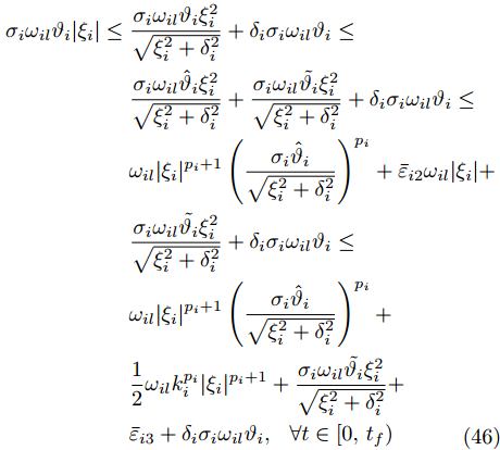
$ \sigma_i\omega_{il}\vartheta_i|\xi_i| $ 放缩为$$ \begin{split} \sigma_i\omega_{il} \vartheta_i|\xi_i|\le\;&\frac{\sigma_i\omega_{il} \vartheta_i\xi_i^2}{\sqrt{\xi_i^2+\delta_i^2}}+\delta_i\sigma_i\omega_{il} \vartheta_i\le\\ &\frac{\sigma_i\omega_{il} \hat{\vartheta}_i\xi_i^2}{\sqrt{\xi_i^2+\delta_i^2}}+\frac{\sigma_i\omega_{il} \tilde{\vartheta_i}\xi_i^2}{\sqrt{\xi_i^2+\delta_i^2}}+\delta_i\sigma_i\omega_{il} \vartheta_i\le\\& \omega_{il} |\xi_{i}|^{p_i+1}\left(\frac{\sigma_i\hat{\vartheta}_i}{\sqrt{\xi_i^2+\delta_i^2}}\right)^{p_i}+\bar{\varepsilon}_{i2}\omega_{il} |\xi_i|+\\ &\frac{\sigma_i\omega_{il} \tilde{\vartheta_i}\xi_i^2}{\sqrt{\xi_i^2+\delta_i^2}}+\delta_i\sigma_i\omega_{il} \vartheta_i\le\\ & \omega_{il} |\xi_{i}|^{p_i+1}\left(\frac{\sigma_i\hat{\vartheta}_i}{\sqrt{\xi_i^2+\delta_i^2}}\right)^{p_i}+\\ &\frac{1}{2}\omega_{il} k_i^{p_i}|\xi_{i}|^{p_i+1}+\frac{\sigma_i\omega_{il} \tilde{\vartheta_i}\xi_i^2}{\sqrt{\xi_i^2+\delta_i^2}}+\\ &\bar{\varepsilon}_{i3}+\delta_i\sigma_i\omega_{il} \vartheta_i,\;\;\forall t\in [0,t_f) \\[-10pt]\end{split} $$ (46) 其中,
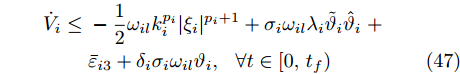
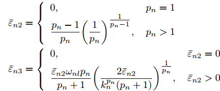
$$ \begin{split} &{{\bar \varepsilon }_{i2}} = \left\{ {\begin{array}{*{20}{l}} {0,}&{{p_i} = 1}\\ {\dfrac{{{p_i} - 1}}{{{p_i}}}{{\left(\dfrac{1}{{{p_i}}}\right)}^{\tfrac{1}{{{p_i} - 1}}}},}&{{p_i} > 1} \end{array}} \right.\\ &{{\bar \varepsilon }_{i3}} = \left\{ {\begin{array}{*{20}{l}} {0,}&{{{\bar \varepsilon }_{i2}} = 0}\\ {\dfrac{{{{\bar \varepsilon }_{i2}}{\omega _{il}}{p_i}}}{{{p_i} + 1}}{{\left(\dfrac{{2{{\bar \varepsilon }_{i2}}}}{{k_i^{{p_i}}({p_i} + 1)}}\right)}^{\tfrac{1}{{{p_i}}}}}},&{{{\bar \varepsilon }_{i2}} > 0} \end{array}} \right. \end{split}$$ 由式(45)和式(46), 可得
$$\begin{split} \dot{V}_i\le\; &-\frac{1}{2}\omega_{il} k_i^{p_i}|\xi_{i}|^{p_i+1}+\sigma_i\omega_{il} \lambda_i\tilde{\vartheta}_i\hat{\vartheta}_i\;+\\ &\bar{\varepsilon}_{i3}+\delta_i\sigma_i\omega_{il} \vartheta_i,\;\;\forall t\in [0,t_f) \end{split} $$ (47) 依据引理2和引理5, 以及Young不等式, 则有
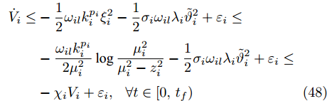
$$ \begin{split} \dot{V}_i\le&-\frac{1}{2}\omega_{il} k_i^{p_i}\xi_{i}^2-\frac{1}{2}\sigma_i\omega_{il} \lambda_i\tilde{\vartheta}_i^2+\varepsilon_i\le\\ &-\frac{\omega_{il} k_i^{p_i}}{2\mu_i^2}\log\frac{\mu_i^2}{\mu_i^2-z_i^{2}}-\frac{1}{2}\sigma_i\omega_{il} \lambda_i\tilde{\vartheta}_i^2+\varepsilon_i\le\\ &-\chi_iV_i+\varepsilon_i,\;\;\forall t\in [0,t_f) \end{split}$$ (48) 其中,
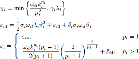
$$ \begin{split} &{\chi _i} = \min \left\{ \frac{{{\omega _{il}}k_i^{{p_i}}}}{{\mu _i^2}},{\gamma _i}{\lambda _i}\right\} \\ &{{\bar \varepsilon }_{i4}} = \frac{1}{2}{\sigma _i}{\omega _{il}}{\lambda _i}\vartheta _i^2 + {{\bar \varepsilon }_{i3}} + {\delta _i}{\sigma _i}{\omega _{il}}{\vartheta _i}\\ &{\varepsilon _i} = \left\{ \begin{array}{*{20}{l}} {{{\bar \varepsilon }_{i4}},}&{{p_i} = 1}\\ {\dfrac{{{\omega _{il}}k_i^{{p_i}}({p_i} - 1)}}{{2({p_i} + 1)}}{{\left(\dfrac{2}{{{p_i} + 1}}\right)}^{\tfrac{2}{{{p_i} - 1}}}} + {{\bar \varepsilon }_{i4}},}&{{p_i} > 1} \end{array} \right. \end{split} $$ 因此, 存在正常数
$ \chi_i^* $ 和$ \varepsilon_i^* $ 满足$$ 0<\chi_i^*\le\chi_i $$ (49) $$ 0<\varepsilon_i\le\varepsilon_i^* $$ (50) 由式(48) ~ (50), 可得
$$ \dot{V}_i\le-\chi_i^*V_i+\varepsilon_i^*,\;\forall t\in [0,t_f) $$ (51) 因此, 对
$ \forall t\in [0,t_f) $ 中, 有$$ \frac{1}{2}\log\frac{\mu_i^2}{\mu_i^2-z_i^{2}}\le V_i\le \varpi_i $$ (52) $$ \frac{\sigma_i\omega_{il} }{2\gamma_i}\tilde{\vartheta}_i^2\le V_i\le \varpi_i\;\; \qquad $$ (53) 其中,
$\varpi_i = \max\{V_i(0),\dfrac{\varepsilon_i^*}{\chi_i^*}\}$ .从式(52)和式(53), 可得
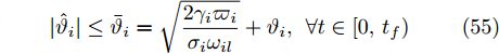
$$ |z_i|\le\bar{\mu}_i = \mu_i\sqrt{1-\exp(-{2}\varpi_i)}<\mu_i $$ (54) $$ |\hat{\vartheta}_i|\le\bar{\vartheta}_i = \sqrt{\frac{2\gamma_i\varpi_i}{\sigma_i\omega_{il}}}+\vartheta_i,\;\forall t\in [0,t_f) $$ (55) 进而可推出, 对
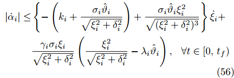
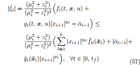
$ \forall t\in [0,t_f) $ ,$ \alpha_i $ 和$ x_{i+1} $ 有界. 接着, 对$ \alpha_i $ 和$ \xi_i $ 分别求导, 可得$$ \begin{split}|\dot{\alpha}_i|\le&\left\{-\left(k_i+\frac{\sigma_i\hat{\vartheta}_i}{\sqrt{\xi_i^2+\delta_i^2}}\right)+\frac{\sigma_i\hat{\vartheta}_i\xi_i^2}{\sqrt{(\xi_i^2+\delta_i^2)^3}}\right\}\dot{\xi}_i+\\ & \frac{\gamma_i\sigma_i\xi_i}{\sqrt{\xi_i^2+\delta_i^2}}\left(\frac{\xi_i^2}{\sqrt{\xi_i^2+\delta_i^2}} -\lambda_i\hat{\vartheta}_i\right),\;\;\forall t\in [0,t_f) \end{split}$$ (56) $$ \begin{split} |\dot{\xi}_i| =\; &\frac{(\mu_i^2+z_i^2)}{(\mu_i^2-z_i^2)^2}\Big(f_i(t,{\boldsymbol{x}},u)\;+\\ &g_i(t,{\boldsymbol{x}},u)[x_{i+1}]^{p_i}-\dot{\alpha}_{i-1}\Big)\le\\ &\frac{(\mu_i^2+z_i^2)}{(\mu_i^2-z_i^2)^2}\Big(\sum\limits_{l = 1}^{j_i}|x_{i+1}|^{q_{il}}\bar{f}_{il}(\bar{{\boldsymbol{x}}}_i)+|\dot{\alpha}_{i-1}|+\\ &\bar{g}_i(\bar{{\boldsymbol{x}}}_{i})|x_{i+1}|^{p_i}\Big),\;\;\forall t\in [0,t_f)\\[-10pt] \end{split} $$ (57) 从式(56)和式(57)可知, 对
$ \forall t\in [0,t_f) $ ,$ \dot{\xi}_i $ 和$ \dot{\alpha}_i $ 亦有界.步骤
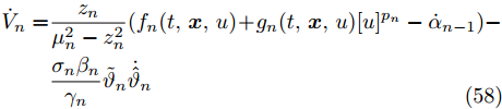
$ {\boldsymbol{n}} $ . 求$ V_n $ 的导数, 可得$$ \begin{split} \dot{V}_n =& \frac{z_n}{\mu_n^2-z_n^{2}}(f_n(t,{\boldsymbol{x}},u) + g_n(t,{\boldsymbol{x}},u)[u]^{p_n}-\dot{\alpha}_{n-1})-\\ &\frac{\sigma_n\beta_n}{\gamma_n}\tilde{\vartheta}_n\dot{\hat{\vartheta}}_n \\[-10pt]\end{split}$$ (58) 类似于式(35)的推导过程, 利用假设1和引理2, 可得
$$ |f_n(t,{\boldsymbol{x}},u)|\le \frac{1}{2}g_n(t,{\boldsymbol{x}},u)|u|^{p_n}+\psi_n(\bar{{\boldsymbol{x}}}_n) $$ (59) 其中,
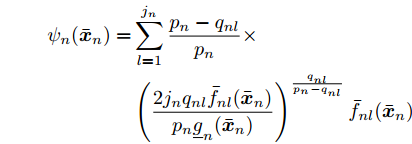
$$ \begin{split} \psi_n(\bar{{\boldsymbol{x}}}_n) = &\sum\limits_{l = 1}^{j_n}\frac{p_n-q_{nl}}{p_n}\times\\ &\left(\frac{2j_nq_{nl}\bar{f}_{nl}(\bar{{\boldsymbol{x}}}_n)}{p_n\underline{g}_n(\bar{{\boldsymbol{x}}}_n)}\right)^{\frac{q_{nl}}{p_n-q_{nl}}}\bar{f}_{nl}(\bar{{\boldsymbol{x}}}_n) \end{split}$$ 由式(59)以及命题1, 可推得
$$ \dot{V}_n\le\omega_n\xi_n[u]^{p_n}+|\xi_n|\nu_n-\frac{\sigma_n\omega_{nl} }{\gamma_n}\tilde{\vartheta}_n\dot{\hat{\vartheta}}_n $$ (60) 其中,
$\omega_n = \dfrac{\underline{g}_n(\bar{{\boldsymbol{x}}}_n)}{2}$ ,$ \nu_n = \psi_n(\bar{{\boldsymbol{x}}}_n)+|\dot{\alpha}_{n-1}| $ .由Part 1可知, 对
$ \forall t\in [0,t_f) $ ,$ |z_j|<\mu_j $ ,$j = 1, \cdots, n$ . 同时, 根据假设1和假设2,$ y_r $ 和$ \dot{y}_r $ 有界, 且$ \bar{f}_{nl} $ ,$ \underline{g}_n $ 和$ \bar{g}_n $ 连续. 此外, 由第$ n-1 $ 步设计可推得$x_1,\cdots, x_n$ ,$ \dot{\alpha}_{n-1} $ 有界,$ \forall t\in [0,t_f) $ . 因此, 运用极值定理, 对$ \forall t\in [0,t_f) $ , 有$$ 0< \omega_{nl}\le \omega_n $$ (61) $$ 0\le \nu_n\le \nu_{nm} $$ (62) 其中,
$ \omega_{nl} $ 和$ \nu_{nm} $ 为未知正常数.利用式(61)和式(62), 有
$$ \begin{split} \dot{V}_n\le\;&\omega_{nl}\xi_n[u]^{p_n}+\nu_{nm}|\xi_n|-\\& \frac{\sigma_n\omega_{nl} }{\gamma_n}\tilde{\vartheta}_n\dot{\hat{\vartheta}}_n,\;\;\forall t\in [0,t_f) \end{split} $$ (63) 根据式(16)和式(17)以及命题1和引理3, 可得
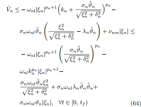
$$ \begin{split} \dot{V}_n\le&-\omega_{nl}|\xi_{n}|^{p_n+1}\Big(k_n+\frac{\sigma_n\hat{\vartheta}_n}{\sqrt{\xi_n^2+\delta_n^2}}\Big)^{p_n}-\\ &\sigma_n\omega_{nl} \tilde{\vartheta}_n\left(\frac{\xi_n^2}{\sqrt{\xi_n^2+\delta_n^2}}-\lambda_n\hat{\vartheta}_n\right)+\nu_{nm}|\xi_n|\le\\ & -\omega_{nl} |\xi_{n}|^{p_n+1}\left(\frac{\sigma_n\hat{\vartheta}_n}{\sqrt{\xi_n^2+\delta_n^2}}\right)^{p_n}-\\ &\omega_{nl} k_n^{p_n}|\xi_{n}|^{p_n+1}-\\ &\frac{\sigma_n\omega_{nl} \tilde{\vartheta}_n\xi_n^2}{\sqrt{\xi_n^2+\delta_n^2}}+\sigma_n\omega_{nl} \lambda_n\tilde{\vartheta}_n\hat{\vartheta}_n+\\ &\sigma_n\omega_{nl} \vartheta_n|\xi_n|,\;\;\forall t\in [0,t_f) \\[-10pt]\end{split}$$ (64) 其中,
$\vartheta_n = \dfrac{\nu_{nm}}{\sigma_n\omega_{nl}}$ .依据引理2和引理4, 式(64)中的项
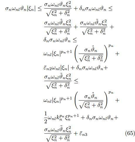
$ \sigma_n\omega_{nl}\vartheta_n|\xi_n| $ 放缩为$$ \begin{split} \sigma_n\omega_{nl} \vartheta_n|\xi_n|\le\;&\frac{\sigma_n\omega_{nl} \vartheta_n\xi_n^2}{\sqrt{\xi_n^2+\delta_n^2}}+\delta_n\sigma_n\omega_{nl} \vartheta_n\le\\ & \frac{\sigma_n\omega_{nl} \hat{\vartheta}_n\xi_n^2}{\sqrt{\xi_n^2+\delta_n^2}}+\frac{\sigma_n\omega_{nl} \tilde{\vartheta}_n\xi_n^2}{\sqrt{\xi_n^2+\delta_n^2}}\;+\\ &\delta_n\sigma_n\omega_{nl} \vartheta_n\le\\ &\omega_{nl} |\xi_n|^{p_n+1}\left(\frac{\sigma_n\hat{\vartheta}_n}{\sqrt{\xi_n^2+\delta_n^2}}\right)^{p_n}+\\ &\bar{\varepsilon}_{n2}\omega_{nl} |\xi_n|+\delta_n\sigma_n\omega_{nl}\vartheta_n+\\ &\frac{\sigma_n\omega_{nl} \tilde{\vartheta}_n\xi_n^2}{\sqrt{\xi_n^2+\delta_n^2}}\le\\ &\omega_{nl} |\xi_n|^{p_n+1}\left(\frac{\sigma_n\hat{\vartheta}_n}{\sqrt{\xi_n^2+\delta_n^2}}\right)^{p_n}+\\ &\frac{1}{2}\omega_{nl} k_n^{p_n}\xi_{n}^{p_n+1}+\delta_n\sigma_n\omega_{nl} \vartheta_n+\\ &\frac{\sigma_n\omega_{nl}\tilde{\vartheta}_n\xi_n^2}{\sqrt{\xi_n^2+\delta_n^2}}+\bar{\varepsilon}_{n3} \end{split} $$ (65) 其中,
$$ \begin{split} &{{\bar \varepsilon }_{n2}} = \left\{ {\begin{array}{*{20}{l}} {0,}&{{p_n} = 1}\\ {\dfrac{{{p_n} - 1}}{{{p_n}}}{{\left(\dfrac{1}{{{p_n}}}\right)}^{\tfrac{1}{{{p_n} - 1}}}},}&{{p_n} > 1} \end{array}} \right.\\ &{{\bar \varepsilon }_{n3}} = \left\{ {\begin{array}{*{20}{l}} {0,}&{{{\bar \varepsilon }_{n2}} = 0}\\ {\dfrac{{{{\bar \varepsilon }_{n2}}{\omega _{nl}}{p_n}}}{{{p_n} + 1}}{{\left(\dfrac{{2{{\bar \varepsilon }_{n2}}}}{{k_n^{{p_n}}({p_n} + 1)}}\right)}^{\tfrac{1}{{{p_n}}}}},}&{{{\bar \varepsilon }_{n2}} > 0} \end{array}} \right. \end{split} $$ 将式(65)代入式(64)中, 得到
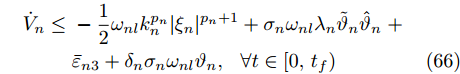
$$ \begin{split} \dot{V}_n\le\;&-\frac{1}{2}\omega_{nl} k_n^{p_n}|\xi_{n}|^{p_n+1}+\sigma_n\omega_{nl} \lambda_n\tilde{\vartheta}_n\hat{\vartheta}_n\;+\\ &\bar{\varepsilon}_{n3}+\delta_n\sigma_n\omega_{nl} \vartheta_n,\;\;\forall t\in [0,t_f) \end{split} $$ (66) 根据引理2和引理5, 以及Young不等式, 可得
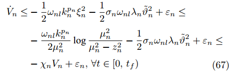
$$ \begin{split} \dot{V}_n\le&-\frac{1}{2}\omega_{nl} k_n^{p_n}\xi_{n}^2-\frac{1}{2}\sigma_n\omega_{nl} \lambda_n\tilde{\vartheta}_n^2+\varepsilon_n\le\\ &-\frac{\omega_{nl} k_n^{p_n}}{2\mu_n^2}\log\frac{\mu_n^2}{\mu_n^2-z_n^{2}}-\frac{1}{2}\sigma_n\omega_{nl} \lambda_n\tilde{\vartheta}_n^2+\varepsilon_n\le\\ &-\chi_nV_n+\varepsilon_n,\forall t\in [0,t_f) \\[-10pt]\end{split} $$ (67) 其中,
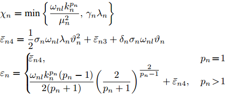
$$ \begin{split} &{\chi _n} = \min \left\{ \frac{{{\omega _{nl}}k_n^{{p_n}}}}{{\mu _n^2}},{\gamma _n}{\lambda _n}\right\} \\ &{{\bar \varepsilon }_{n4}} = \frac{1}{2}{\sigma _n}{\omega _{nl}}{\lambda _n}\vartheta _n^2 + {{\bar \varepsilon }_{n3}} + {\delta _n}{\sigma _n}{\omega _{nl}}{\vartheta _n}\\ &{\varepsilon _n} = \left\{ {\begin{array}{*{20}{l}} {{{\bar \varepsilon }_{n4}},}&{{p_n} = 1}\\ {\dfrac{{{\omega _{nl}}k_n^{{p_n}}({p_n} - 1)}}{{2({p_n} + 1)}}{{\left(\dfrac{2}{{{p_n} + 1}}\right)}^{\tfrac{2}{{{p_n} - 1}}}} + {{\bar \varepsilon }_{n4}},}&{{p_n} > 1} \end{array}} \right. \end{split} $$ 因此, 存在正常数
$ \chi_n^* $ 和$ \varepsilon_n^* $ , 使得$$ 0<\chi_n^*\le \chi_n $$ (68) $$ 0<\varepsilon_n\le\varepsilon_n^* \; $$ (69) 根据式(67) ~ (69), 可得
$$ \dot{V}_n\le-\chi_n^*V_n+\varepsilon_n^*,\;\;\forall t\in [0,t_f) $$ (70) 因此, 对
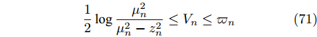
$ \forall t\in [0,t_f) $ , 有$$ \frac{1}{2}\log\frac{\mu_n^2}{\mu_n^2-z_n^{2}}\le V_n\le \varpi_n $$ (71) $$ \frac{\sigma_n\omega_{nl} }{2\gamma_n}\tilde{\vartheta}_n^2\le V_n\le \varpi_n\;\;\;\;\;\;\; $$ (72) 其中,
$\varpi_n = \max\{V_n(0),\dfrac{\varepsilon_n^*}{\chi_n^*}\}$ .由式(71)和式(72), 可得
$$ |z_n|\le \bar{\mu}_n = \mu_n\sqrt{1-\exp(-{2}\varpi_n)}<\mu_n\;\;\;\;\; $$ (73) $$ |\hat{\vartheta}_n|\le\sqrt{\bar{\vartheta}_n = \frac{2\gamma_n\varpi_n}{\sigma_n\omega_{nl}}}+\vartheta_n,\;\; \forall t\in [0,t_f) $$ (74) 故可推出, 对
$ \forall t\in [0,t_f) $ ,$ u $ 有界.由步骤 1 ~
$n $ 可知, 存在紧子集$\Xi' = [-\bar{\mu}_1,\bar{\mu}_1]\,\times \cdots\times [-\bar{\mu}_n, \bar{\mu}_n]\times [-\bar{\vartheta}_1,\bar{\vartheta}_1]\times\cdots\times[-\bar{\vartheta}_n,\bar{\vartheta}_n]\subset \Xi$ , 使得闭环系统在$ [0,t_f) $ 上存在唯一解$ {\boldsymbol{\eta}}(t)\in \Xi' $ . 根据引理1, 可得:$ t_f = +\infty $ , 即, 对$ \forall t \in [0,+\infty) $ ,$|z_i| < \mu_i$ ,$i = 1, \cdots,n$ .Part 3. 重复Part 2中的步骤1 ~ n, 可得
$x_1,\cdots, x_n$ ,$\alpha_1,\cdots,\alpha_{n-1}$ 和$ u $ 均有界,$ \forall t \in [0,+\infty) $ . 另外, 从式(54)可知, 通过减小$ \mu_1 $ 和$ \varpi_1 $ 可将输出跟踪误差$ z_1 $ 收敛到任意小的残差集. □注 4. 不同于文献[20-25]中提出的控制方案, 本文采用积分反推技术和障碍李雅普诺夫方法解决了高阶非线性系统中幂次未知和系统函数不确定的问题, 且所设计控制策略不依赖于未知幂次的上界信息.
3. 仿真算例
为了验证本文所提控制算法的有效性与通用性, 考虑如下两个高阶非线性系统
$$ {\Sigma _1}:\left\{ \begin{aligned} &{{{\dot x}_1} = {f_{1,{\Sigma _1}}} + {g_{1,{\Sigma _1}}}{{[{x_2}]}^{{p_1}}}}\\ &{{{\dot x}_2} = {f_{2,{\Sigma _1}}} + {g_{2,{\Sigma _1}}}{{[u]}^{{p_2}}}}\\ &{y = {x_1}} \end{aligned} \right. $$ (75) $$ {\Sigma _2}:\left\{ \begin{aligned} &{{{\dot x}_1} = {f_{1,{\Sigma _2}}} + {g_{1,{\Sigma _2}}}{{[{x_2}]}^{{p_1}}}}\\ &{{{\dot x}_2} = {f_{2,{\Sigma _2}}} + {g_{2,{\Sigma _2}}}{{[u]}^{{p_2}}}}\\ &{y = {x_1}} \end{aligned} \right. $$ (76) 其中,
$p_1 = {5}/{3}$ ,$p_2 ={7}/{3}$ ,$ f_{1,\Sigma_1} = x_1\cos (t) $ ,$g_{1,\Sigma_1} = 3+ 0.5\sin (t)$ ,$f_{2,\Sigma_1} = x_1+2\sin (x_1x_2)$ ,$g_{2,\Sigma_1} = 2+ 0.1\sin (t)$ ,$f_{1,\Sigma_2} \;= \;(0.5x_1\; +\; 1)\cos (t)$ ,$g_{1,\Sigma_2} = 2 + 0.1\sin (t)$ ,$f_{2,\Sigma_2} = \cos (x_1 )\exp(2x_2\sin (x_1 )) + x_1x_2\sin (t)$ ,$g_{2,\Sigma_2} = 1$ , 期望参考信号$y_r(t) = \dfrac{\pi}{2}(1 - \exp( -0.1t^2)) \sin (t)$ .在仿真中, 系统
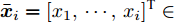
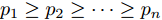
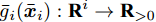
$ \Sigma_i $ 和自适应参数$ \hat{\vartheta}_i $ 的初始值设置为$ [x_1(0),x_2(0)]^{\rm{T}} = [-0.5,0.4]^{\rm{T}} $ ,$ \hat{\vartheta}_i(0) = 0 $ ,$i = 1,2$ . 控制器参数$ k_1 = 2 $ ,$ k_2 = 1 $ ,$ \mu_1 = 4 $ ,$ \mu_2 = 2 $ ,$ \sigma_1 = 3 $ ,$ \sigma_2 = 2 $ ,$ \gamma_1 = 2 $ ,$ \gamma_2 = 3 $ ,$ \delta_1 = \delta_2 = 0.01 $ 和$ \lambda_1 = \lambda_2 = 0.002 $ , 其中,$ \mu_1 = 4>|z_1(0)| = 0.5 $ ,$\mu_2 = 2 > |z_2(0)| = {106}/{315}$ . 系统$ \Sigma_1 $ 和$ \Sigma_2 $ 的仿真结果如图2 ~ 4所示. 图2刻画了输出跟踪误差$ y-y_r $ 的变化情况, 图3给出系统的控制信号$ u $ , 图4描述了自适应参数$ \hat{\vartheta}_1 $ 和$ \hat{\vartheta}_2 $ . 从仿真结果可以看出, 本文所提自适应控制策略既能使系统$ \Sigma_1 $ 和$ \Sigma_2 $ 的输出跟踪误差收敛到原点附近的较小邻域内, 又能确保闭环系统的所有信号有界.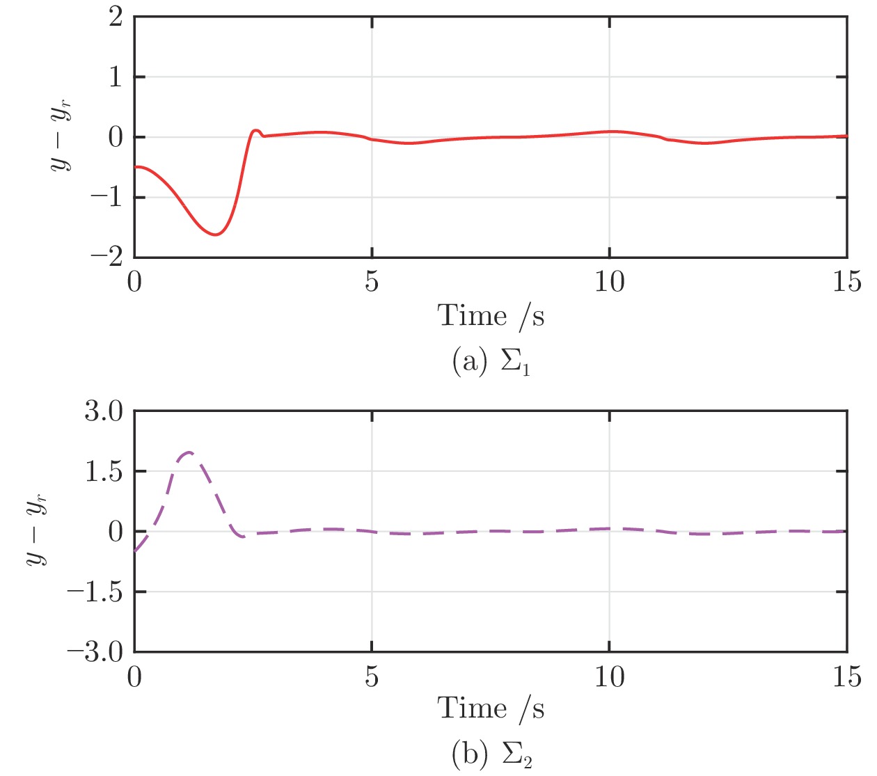 图 2 系统
$\Sigma_1$ 和$\Sigma_2$ 的输出跟踪误差$y-y_r$ Fig. 2 Output tracking errors$y-y_r$ of systems$\Sigma_1$ and$\Sigma_2$ 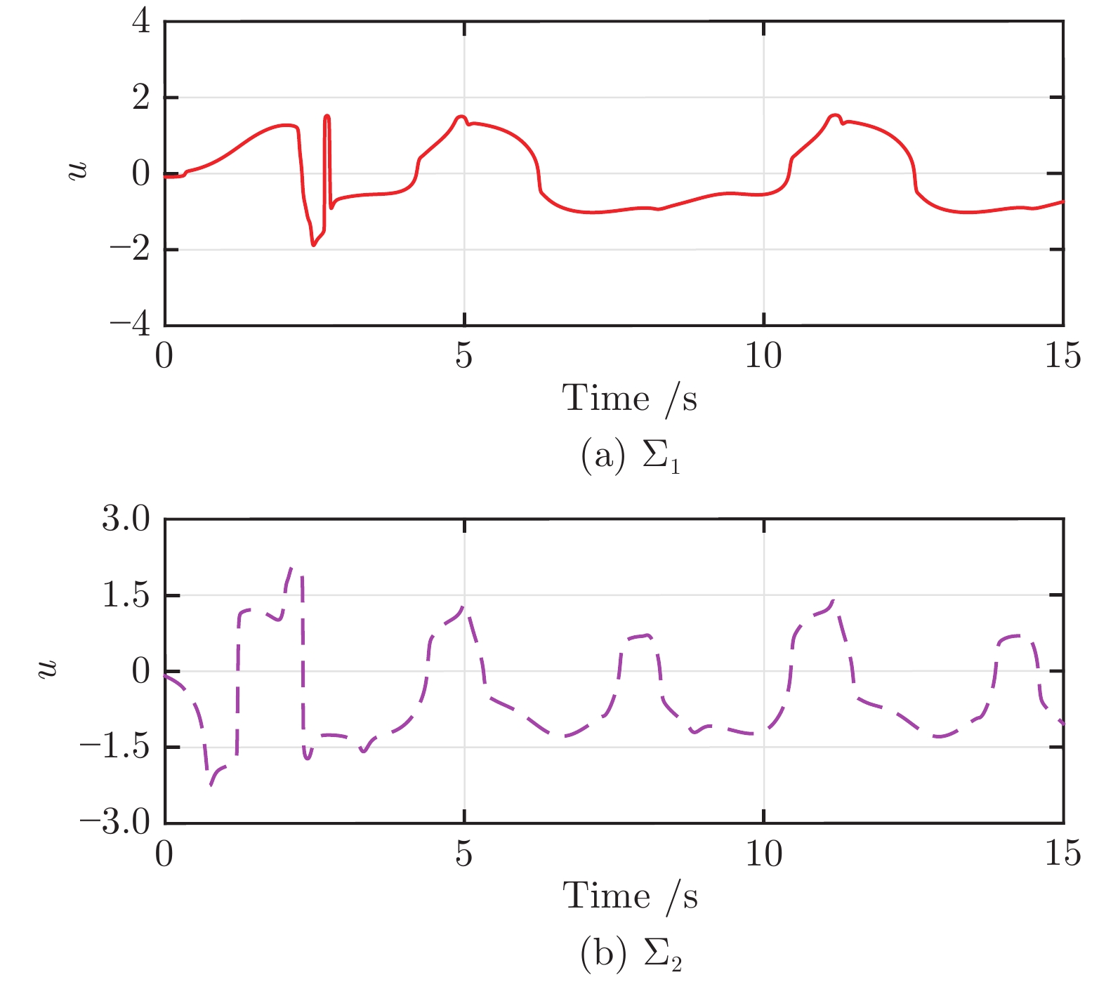 图 3 系统
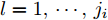
$\Sigma_1$ 和$\Sigma_2$ 的控制信号$u$ Fig. 3 Control signals$u$ of systems$\Sigma_1$ and$\Sigma_2$  图 4 系统
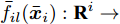
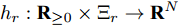
$\Sigma_1$ 和$\Sigma_2$ 的自适应参数$\hat{\vartheta}_1$ 和$\ \hat{\vartheta}_2$ Fig. 4 Adaptive parameters$\hat{\vartheta}_1$ and$\hat{\vartheta}_2$ of systems$\Sigma_1$ and$\Sigma_2$ 为进一步验证本文控制算法的幂次无关特性, 在系统初始值与控制器参数不变的条件下, 对具有不同幂次
$ p_1 $ 和$ p_2 $ 的系统$ \Sigma_1 $ 进行仿真测试. 仿真结果如图5和图6所示. 图5为系统$ \Sigma_1 $ 在不同幂次$ p_1 $ 和$ p_2 $ 条件下的输出跟踪误差$ y-y_r $ , 图6为相应的控制信号$ u $ . 仿真结果表明, 在不同幂次条件下, 该控制器仍然可以保证闭环系统获得良好的控制性能. 图 5 系统
$\Sigma_1$ 在不同幂次下的跟踪误差$y-y_r$ Fig. 5 Output tracking errors$y-y_r$ of system$\Sigma_1$ under various powers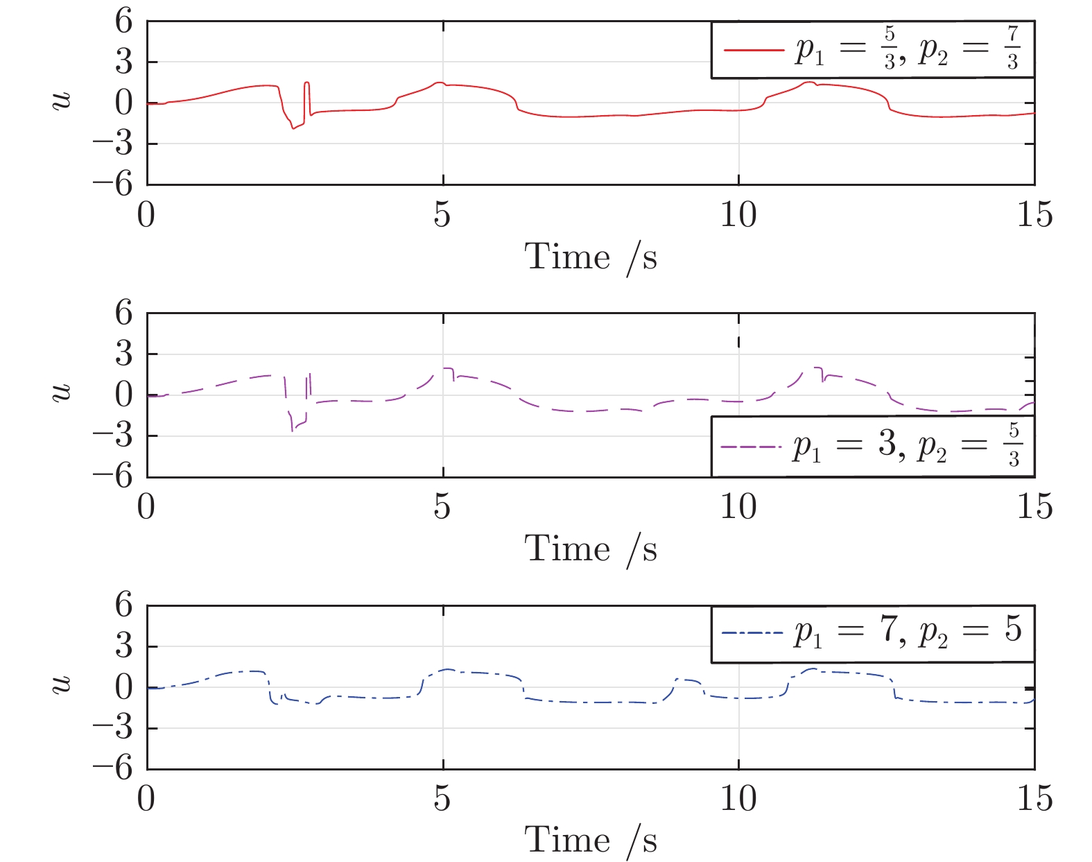 图 6 系统
$\Sigma_1$ 在不同幂次下的控制信号$u$ Fig. 6 Control signals$u$ of system$\Sigma_1$ under various powers4. 结束语
针对一类具有未知幂次的高阶不确定非线性系统, 提出了一种基于障碍李雅普诺夫函数的自适应控制算法. 在无需知晓系统函数先验知识的条件下, 所提控制算法有效克服了系统幂次未知与模型不确定带来的技术挑战. 该算法的显著特点是所设计的自适应控制器均与系统幂次无关. 最后, 仿真结果验证了本文控制算法的有效性与通用性.
今后的研究方向包括将本文所提方法推广到具有未知幂次的高阶非线性系统的输出反馈控制设计[34]. 此外, 为验证本文方法的实用性, 将本文所提控制策略应用于实际系统[35]亦是我们未来研究的目标.
-

图 1 被质疑造假的日本人质视频截图
Fig. 1 The photo of Japanese hostages which is considered as a spliced image
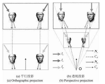
图 3 平行投影和透视投影对光照估计的影响示意图
Fig. 3 The influences of the projection methods on the lighting estimation
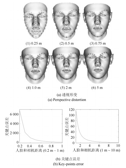
图 4 人脸透视形变程度随人脸到相机距离变化的情况
Fig. 4 The influences of the distance from the face to the camera on the facial perspective distortion
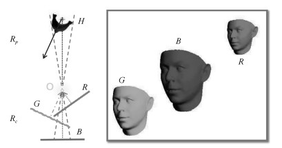
图 6 固定人脸和相机光心, 人脸的照片姿态就保持不变, 不随相机焦距变化和姿态旋转而变化
Fig. 6 The poses of the face in the photo remain the same once the face and the optical center are fixed

图 9 晴天下拍摄的一个足球队的真实照片
Fig. 9 A pristine photo of a football team taken on a sunny day to verify our proposed approach
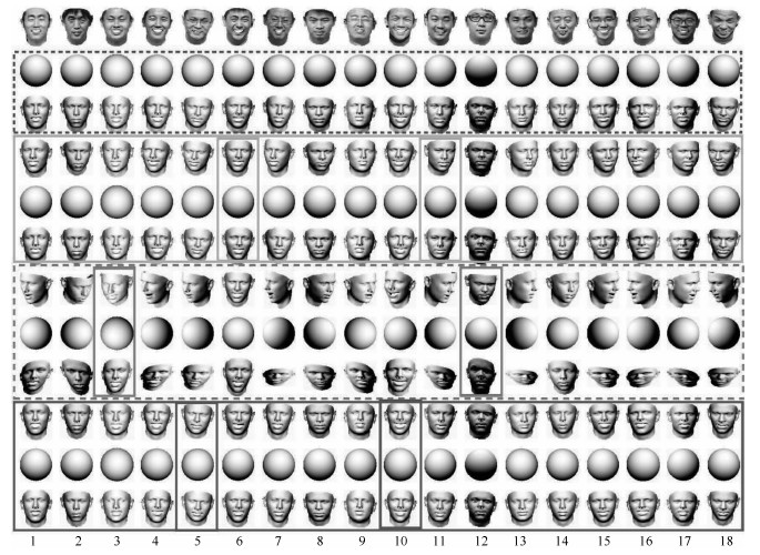
图 11 图 9中18名队员的三维人脸模型和投影光照渲染球, 以及三组通过不同人脸估计的透视参数对应的人脸空间姿态、空间光照渲染球及重新投影的人脸透视模型对比
Fig. 11 The 3D face models and projected lighting of the 18 players in Fig. 9, and three groups of spatial pose, spatial lighting and re-projected face model under the estimated perspective parameters using three different pairs of faces
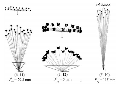
图 12 根据人脸(6, 11)、(3, 12)、(5, 10)优化得到的参数估计出在人脸空间分布(上方为正视图, 下方为俯视图)
Fig. 12 The estimated spatial poses of 18 human faces according to the optimized parameters of human faces (6, 11), (3, 12) and (5, 10), respectively (The first row is the face view, and the second row is the top view of the faces)
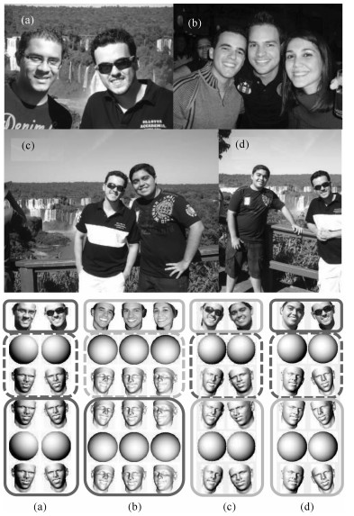
图 13 对DSO-1数据集中的四幅样本图像的检测结果. (a)$\sim$(d)分别是对拼接图像正确检测, 对原始图像错误报警, 对原始图像正确检测, 对拼接图像错误检测
Fig. 13 The detection results of our method on four sample images in the DSO-1 dataset. (a) $\sim$ (d) are respectively a correct detection for splicing image, a false alarm for pristine image, a correct detection for pristine image and a miss detection for splicing image
表 1 实验中各案例相关参数列表及判断意见
Table 1 Comparisons of relevant parameters and corresponding judgment opinions of each case in the experiment
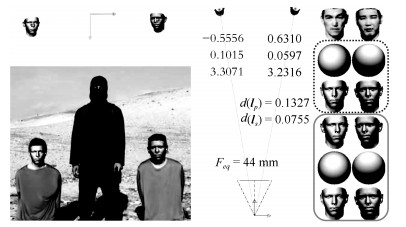
人脸组合 $d(\boldsymbol{l}_{pij})$ 意见1 $d(\boldsymbol{l}_{sij})$ 意见2 $F_{eq}$ (mm)/理论焦距 $D_{HH}\, {\rm (m)}/D_{OH}$ (m) $I_{re}$ 意见3 实际 图 10(6, 11) 0.0219 不一致 0.0001 一致 29.3/中 0.50合理/4.00合理 接近 合理 真实 图 10(3, 12) 0.3508 不一致 0.3009 不一致 5/中 0.18过近/1.00过近 严重 不合理 篡改 图 10(5, 10) 0.0063 一致 0.0098 一致 115/中 1.00过远/15.00过远 接近 不合理 真实 图 14(a) 0.2463 不一致 0.2371 不一致 125/中 2.00过远/20.00过远 接近 不合理 篡改 图 14(b) 0.0093 一致 0.0065 一致 94/短 0.60过远/18.00过远 接近 不合理 真实 图 14(c) 0.0635 不一致 0.0167 一致 20.2/中 0.24合理/1.00合理 接近 合理 真实 图 14(d) 0.1065 不一致 0.0361 不一致 34/中 0.69合理/1.70合理 接近 合理 篡改 图 1 0.1327 不一致 0.0755 不一致 44/中 1.20过远/3.00合理 接近 合理 待检  下载: 导出CSV
-
[1] Rossler A, Cozzolino D, Verdoliva L, Riess C, Thies J, Niessner M. FaceForensics++: learning to detect manipulated facial images. arXiv preprint, 2019. arXiv: 1901.08971 [2] Farid H. Creating and Detecting Doctored and Virtual Images: Implications to the Child Pornography Prevention Act. Technical Report TR2004-518, Department of Computer Science, Dartmouth College, USA, 2004. [3] Farid H. A survey of image forgery detection. IEEE Signal Processing Magazine, 2009, 26(2): 16-25 [4] Popescu A C, Farid H. Exposing digital forgeries by detecting traces of resampling. IEEE Transactions on Signal Processing, 2005, 53(2): 758-767 doi: 10.1109/TSP.2004.839932 [5] Luo W, Huang J, Qiu G. JPEG error analysis and its applications to digital image forensics. IEEE Transactions on Information Forensics and Security, 2010, 5(3): 480-491 doi: 10.1109/TIFS.2010.2051426 [6] Gou H, Swaminathan A, Wu M. Noise features for image tampering detection and steganalysis. In: Proceedings of the 2007 IEEE International Conference on Image Processing. San Antonio, TX, USA: IEEE, 2007. 97-100 https://ieeexplore.ieee.org/document/4379530 [7] Zhou P, Han X, Morariu V I, Davis L S. Learning rich features for image manipulation detection. In: Proceedings of the IEEE Conference on Computer Vision and Pattern Recognition. Salt Lake City, USA: IEEE, 2018. 1053-1061 https://www.researchgate.net/publication/325143175_Learning_Rich_Features_for_Image_Manipulation_Detection [8] Gloe T, Franz E, Winkler A. Forensics for flatbed scanners. In: Proceedings of SPIE 6505, Security, Steganography, and Watermarking of Multimedia Contents IX. California, USA: International Society for Optics and Photonics, 2007. 650511 [9] Kakar P, Sudha N, Ser W. Exposing digital image forgeries by detecting discrepancies in motion blur. IEEE Transactions on Multimedia, 2011, 13(3): 443-452 doi: 10.1109/TMM.2011.2121056 [10] Farid H, Bravo M J. Image forensic analyses that elude the human visual system. In: Proceedings of SPIE 7541, Media Forensics and Security Ⅱ. California, USA: International Society for Optics and Photonics, 2010. 754106 doi: 10.1117/12.837788 [11] Peng B, Wang W, Dong J, Tan T. Image forensics based on planar contact constraints of 3D objects. IEEE Transactions on Information Forensics and Security, 2018, 13(2): 377-392 doi: 10.1109/TIFS.2017.2752728 [12] Carvalho T J D, Riess C, Angelopoulou E, Pedrini H, Rocha A D R. Exposing digital image forgeries by illumination color classification. IEEE Transactions on Information Forensics and Security, 2014, 18(6): 1182-1194 http://www.wanfangdata.com.cn/details/detail.do?_type=perio&id=Doaj000003806817 [13] Johnson M K, Farid H. Exposing digital forgeries through specular highlights on the eye. In: Proceedings of International Workshop on Information Hiding. Berlin, Heidelberg, Germany: Springer, 2007. 311-325 doi: 10.1007/978-3-540-77370-2_21 [14] Liu Q, Cao X, Chao D, Guo X. Identifying image composites through shadow matte consistency. IEEE Transactions on Information Forensics and Security, 2011, 6(3): 1111-1122 doi: 10.1109/TIFS.2011.2139209 [15] Kee E, O0Brien J F, Farid H. Exposing photo manipulation with inconsistent shadows. ACM Transactions on Graphics, 2013, 32(3): 28 http://www.wanfangdata.com.cn/details/detail.do?_type=perio&id=33fd7688600a6dd746ed39aa3727a855 [16] Kee E, O0Brien J F, Farid H. Exposing photo manipulation from shading and shadows. ACM Transactions on Graphics, 2014, 33(5): 1-21 https://www.mendeley.com/catalogue/exposing-photo-manipulation-shading-shadows/ [17] Johnson M K, Farid H. Exposing digital forgeries by detecting inconsistencies in lighting. In: Proceedings of the 7th workshop on Multimedia and security. NewYork, NY, USA: ACM Press, 2005. 1-10 https://www.mendeley.com/catalogue/exposing-digital-forgeries-detecting-inconsistencies-lighting/ [18] Carvalho T, Farid H, Kee E R. Exposing photo manipulation from user-guided 3d lighting analysis. In: Proceedings of SPIE Symposium on Electronic Imaging. California, USA: International Society for Optics and Photonics, 2015. 940902 [19] Johnson M K, Farid H. Exposing digital forgeries in complex lighting environments. IEEE Transactions on Information Forensics and Security, 2007, 2(3): 450-461 doi: 10.1109/TIFS.2007.903848 [20] Kee E, Farid H. Exposing digital forgeries from 3-D lighting environments. In: Proceedings of IEEE International Workshop on Information Forensics and Security. Seattle, USA: IEEE, 2010. 1-6 [21] Peng B, Wang W, Dong J, Tan T. Optimized 3D lighting environment estimation for image forgery detection. IEEE Transactions on Information Forensics and Security, 2017, 12(2): 479-494 doi: 10.1109/TIFS.2016.2623589 [22] 孙鹏, 郎宇博, 樊舒, 沈喆, 彭思龙, 刘磊.图像拼接篡改的自动色温距离分类检验方法.自动化学报, 2018, 44(7): 171-182 http://www.aas.net.cn/CN/abstract/abstract19318.shtmlSun Peng, Lang Yu-Bo, Fan Shu, Shen Zhe, Peng Si-Long, Liu Lei. Detection of image splicing manipulation by automated classification of color temperature distance. Acta Automatica Sinica, 2018, 44(7): 171-182 http://www.aas.net.cn/CN/abstract/abstract19318.shtml [23] 朱叶, 申铉京, 陈海鹏.基于彩色LBP的隐蔽性复制–粘贴篡改盲鉴别算法.自动化学报, 2017, 43(3): 390-397 http://www.aas.net.cn/CN/abstract/abstract19017.shtmlZhu Ye, Shen Xuan-Jing, Chen Hai-Peng. Covert copy-move forgery detection based on color LBP. Acta Automatica Sinica, 2017, 43(3): 390-397 http://www.aas.net.cn/CN/abstract/abstract19017.shtml [24] Blanz V, Vetter T. A morphable model for the synthesis of 3D faces. In: Proceedings of the 26th annual conference on Computer graphics and interactive techniques. NewYork, USA: ACM, 1999. 187-194 [25] Zhu X, Lei Z, Yan J, Yi D, Li S Z. High-fidelity pose and expression normalization for face recognition in the wild. In: Proceedings of the IEEE Conference on Computer Vision and Pattern Recognition. Boston, USA: IEEE, 2015. 787-796 [26] King D E. Dlib-ml: a machine learning toolkit. Journal of Machine Learning Research, 2009, 10(Jul): 1755-1758 https://core.ac.uk/display/21155954 [27] Phong B T. Illumination for computer generated pictures. Communications of the Acm, 1975, 18(6): 311-317 doi: 10.1145/360825.360839 [28] Ramamoorthi R, Hanrahan P. On the relationship between radiance and iIrradiance: determining the illumination from images of a convex lambertian object. Journal of the Optical Society of America A, 2001, 18(10): 2448-2459 doi: 10.1364/JOSAA.18.002448 [29] Basri R, Jacobs D. Lambertian reflectance and linear subspaces. IEEE Transactions on Pattern Analysis and Machine Intelligence, 2003, 25(2): 218-233 doi: 10.1109/TPAMI.2003.1177153 [30] Zhang Z. A flexible new technique for camera calibration. IEEE Transactions on Pattern Analysis and Machine Intelligence, 2000, 22(11): 1330-1334 doi: 10.1109/34.888718 [31] Zhou W, Kambhamettu C. Estimation of illuminant direction and intensity of multiple light sources. In: Proceedings of European conference on computer vision. Berlin, Heidelberg, Germany: Springer, 2002. 206-220 期刊类型引用(9)
1. 尹宏伟,杭雨晴,胡文军. 融合异常检测与区域分割的高效K-means聚类算法. 郑州大学学报(工学版). 2024(03): 80-88 .  百度学术
百度学术2. 黄鹤,黄佳慧,刘国权,王会峰,高涛. 采用混合策略联合优化的模糊C-均值聚类信息熵点云简化算法. 西安交通大学学报. 2024(07): 214-226 . 百度学术3. 高瑞贞,王诗浩,王皓乾,张京军,李志杰. 基于图注意力机制的三维点云感知. 中国测试. 2024(07): 155-162 . 百度学术4. 邢建平,殷煜昊. 基于三维重建外点剔除的船舶航迹自适应修正. 舰船科学技术. 2024(14): 162-165 . 百度学术5. 梁循,李志莹,蒋洪迅. 基于图的点云研究综述. 计算机研究与发展. 2024(11): 2870-2896 . 百度学术6. 黄鹤,温夏露,杨澜,王会峰,高涛,茹锋. 基于疯狂捕猎秃鹰算法的K均值互补迭代聚类优化. 浙江大学学报(工学版). 2023(11): 2147-2159 . 百度学术7. 胡建平,刘凯,郭新宇,吴升,温维亮. 自适应加权算子结合主曲线提取玉米叶片点云骨架. 农业工程学报. 2022(02): 166-174 . 百度学术8. 任彪,陆玲. 基于PCL三维点云花瓣分割与重建. 现代电子技术. 2022(12): 149-154 . 百度学术9. 吴艳娟,王健,王云亮. 基于骨架提取算法的作物茎秆识别与定位方法. 农业机械学报. 2022(11): 334-340 . 百度学术其他类型引用(15)
-


 下载:
下载:


计量
- 文章访问数: 1554
- HTML全文浏览量: 452
- PDF下载量: 136
- 被引次数: 24
