

-
摘要: 人脸活体检测是为了提高人脸识别系统安全性而需要重点研究的问题.本文首先从人脸活体检测的问题出发, 分个体、类内、类间三个层面对人脸活体检测存在的困难与挑战进行了阐述分析.接下来, 本文以算法使用的分类线索为主线, 分类别对人脸活体检测算法及其优缺点进行了梳理和总结.之后, 本文就常用人脸活体检测数据集的特点、数据量、数据多样性等方面进行了对比分析, 对算法评估常用的性能评价指标进行了阐述, 总结分析了代表性人脸活体检测方法在照片视频类数据集CASIA-MFSD、Replay-Attack、Oulu-NPU、SiW以及面具类数据集3DMAD、SMAD、HKBU-MARsV2上的实验性能.最后本文对人脸活体检测未来可能的发展方向进行了思考和探讨.Abstract: Face anti-spoofing is an important research field for ensuring the security of face recognition system. In this paper, we first discuss the difficulties and challenges in the development of face anti-spoofing. Then we take the classification clues utilized by the methods as the main line to review the achievements in the study of face anti-spoofing. Next, we analyze the characteristics, data volume and data diversity of commonly used face anti-spoofing datasets. The evaluation metrics of performances commonly used in algorithm evaluation are expounded. We summarize and analyze the performances of representative face anti-spoofing methods on CASIA-MFSD, Replay-Attack, Oulu-NPU, SiW, 3DMAD, SMAD and HKBU-MARsV2 datasets. Finally, we discuss the future development direction of face anti-spoofing.
-
Key words:
- Face anti-spoofing /
- computer vision /
- face recognition /
- deep learning /
- feature representations
1) 本文责任编委 刘青山 -
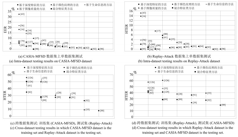
图 5 各类人脸活体检测方法性能分布图
Fig. 5 Performance comparison of different category of face anti-spoofing methods
表 1 主流人脸活体检测方法总览
Table 1 Brief overview of face anti-spoofing methods
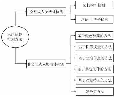
一级类别 二级类别 分类特征 防范的假体人脸 算法优点 算法缺点 交互式人脸活体检测 基于随机动作的方法 用户配合的动作: 点头、抬头、眨眼、闭眼、遮挡眼睛、扬眉、皱眉、笑脸、吐舌头、张嘴[8, 12] 照片、视频 对二维类假体人脸准确率高, 通用性强 需要用户配合, 用户体验差, 不能防止眼部、嘴部挖洞的面具攻击, 适用范围窄 基于唇语声音混合的方法 朗读一个数字串、一段文字时的唇语与声音[10-11] 非交互式人脸活体检测 基于图像纹理的方法 LBP、HOG、Gabor等描述符从灰度图中抽取的灰度纹理特征[15-17, 21, 23, 30-33] 照片、视频、面具 容易实现, 计算量少, 单张图片可预测结果, 速度快 容易被拍摄设备、光照条件、图像质量影响, 跨数据集通用能力不强 LBP、LPQ等描述符从HSV, YCbCr颜色空间图像中抽取的颜色纹理特征[20, 35, 39] 基于图像质量的方法 手工设计特征抽取图像镜面反射、颜色分布、清晰度方面的图像质量特征[43-45] 照片、视频 针对单类假体人脸的跨数据集通用能力相对强, 速度快 需要根据假体人脸的类别设计具体特征, 跨假体类型的通用能力不强, 需要高质量图像, 难以抵御高清哑光照片视频攻击 基于生命信息的方法 光流法、运动成分分解检测活体不自主地眨脸部、唇部的微运动[48, 51-52, 56] 照片 对照片类假体人脸准确率高, 通用性高 需要视频为输入
计算量大, 速度慢
难以防范视频攻击
对假体制造的微运动鲁棒性不强远程光学体积描记术(rPPG)信息检测待测 面具 特定约束条件下准确率高 需要视频为输入
鲁棒性不强, 受外界光照、个体运动的影响大基于其他硬件的方法 近红外图像特征[62-68] 照片、视频、面具 准确率高 需要增加新的昂贵硬件
设备采集、处理图像的时间增加短波红外图像特征[69] 热红外图像特征[70]
400 nm至1 000 nm的多个波段图像特征[71-72]
光场图像信息[73-74]
深度图像信息[75-78]基于深度特征的方法 从头训练CNN抽取深度特征分类[79-80, 83]、利用预训练的ResNet-50、VGG等模型抽取特征[84−85, 87] 照片、视频、面具 相对来说, 准确率较高 模型参数多, 计算量大, 训练时间长
过拟合问题
对数据量和数据丰富性上有高要求深度特征与手工特征融合[85, 95-97] 三维卷积抽取时空深度特征[93-94] 混合特征类方法 纹理信息和运动生命信息的混合[17-19, 25, 85, 93-94, 97, 99-101] 照片、视频、面具 融合多特征的优点
提升识别准确率和通用性计算量、存储增大, 相对识别时间增长
算法实现和维护的工作量增加纹理信息和人脸结构信息的混合[76, 80, 83, 98, 102] 人脸结构信息与运动生命信息的混合[89] 图像质量与运动生命信息的混合[95] 背景信息[27]和其他特征的混合[79, 81, 84, 87, 93, 98, 100]  下载: 导出CSV
表 2 主流人脸活体检测数据集总览
Table 2 Brief overview of face anti-spoofing datasets
数据集 年份 假体人脸 个体数 数据量 姿态、表情、光照等录制场景 录制设备与图像分辨率 NUAA[116] 2010 三种打印照片 15 12 641张图像 三个不同光照的外界环境 网络摄像头–可见光图像640 × 480像素 Yale Recaptured[33] 2011 LCD屏显示的照片 10 2 560张图像 64种不同光照 Kodak C813 8.2与Samsung Omnia i900的摄像头–裁剪后的灰度图 64 × 64像素 Print-Attack Database[117] 2011 手持照片、固定照片 50 200个视频 两种不同光照 可见光图像
苹果笔记本内置摄像头– 320 × 240像素CASIA MFSD[34] 2012 弯曲照片、挖眼照片、视频 50 600个视频 室内光照 可见光图像
使用时间长的USB摄像头– 640 × 480像素; 新USB摄像头– 480 × 640像素; Sony NEX-5摄像头– 1 920 × 1 080像素Replay Attack[16] 2012 手持或者固定的照片与视频 50 1 300个视频 两种不同光照 可见光图像
苹果笔记本内置摄像头– 320 × 240像素MSU MFSD[45] 2015 高分辨率照片与视频 35 280个视频 一个场景 可见光图像
MacBook Air 13内置摄像头– 640 × 480像素
Google Nexus 5前置摄像头– 720 × 480像素UVAD[31] 2015 6种设备拍摄的人脸视频 404 17 076个视频 不同背景光照的室内室外场景 索尼摄像头–可见光图像1 366 × 768像素 REPLAY MOBILE[118] 2016 高分辨率照片与视频 40 1 200个视频 五种不同光照 iPad Mini2 (iOS) 以及LG-G4
前置摄像头–可见光图像720 × 1 280像素MSU USSA[119] 2016 高分辨率照片与视频 1 000 9 000张 一个场景 可见光图像
Google Nexus 5前置摄像头– 1 280 × 960像素; 后置摄像头– 3 264 × 2 448像素Oulu-NPU[120] 2017 照片与视频 55 5 940个视频 三种不同光照场景 六种智能手机的前置摄像头–可见光图像1 920 × 1 080像素 SiW[89] 2018 高低两种分辨率的照片, 弯曲照片与高分辨率视频 165 4 478个视频 活体人脸录制了距离、姿态、表情、光照差异 Canon EOST6, Logitech C920摄像头–可见光图像1 920 × 1 080像素 GUC LiFFAD[21] 2015 激光、喷墨打印的照片, iPad显示的照片 80 4 826张图像 不同焦距的图像, 室内室外场景 光场相机 Msspoof[121] 2016 可见光与近红外光谱的黑白照片 22 4 704张图片 7种不同的室内室外环境 uEye摄像头以及近红外滤波器
可见光与近红外图像– 1 280 × 1 024像素EMSPAD[122] 2017 激光打印的照片, 喷墨打印的照片 50 10 500张图像 2个场景 多光谱摄像头7个波段的图像
裁剪对齐后120 × 120像素3DMAD[37] 2013 定制三维人脸面具 17 76 500张图像 3种不同场景 Kinect深度摄像头–深度图 640 × 480像素; 可见光摄像头–可见光图像640 × 480像素 HKBU MARsV2[123] 2016 两种三维人脸面具 12 1 008个视频 7种不同光照 可见光图像, 三种传统摄像头:
Logitech C920网络摄像头– 1 280 × 720像素; 工业摄像头– 800 × 600像素; Canon EOS M3-1 280 × 720像素; 可见光图像, 4种移动设备摄像头:
Nexus 5, iPhone6, Samsung S7, Sony Tablet S;SMAD[92] 2017 硅胶三维人脸面具 – 130个视频 不同光照, 不同录制背景环境 – MLFP[124] 2017 挖去眼部的二维照片, 乳胶三维人脸面具 10 1 350个视频 室内室外场景 Android智能手机–可见光图像1 280 × 720像素; FLIR ONE热像仪安卓版–热红外图像640 × 480像素; 微软Kinect –近红外图像424 × 512像素
下载: 导出CSV
表 3 CASIA-MFSD与Replay-Attack数据集单数据集测试性能数据(%)
Table 3 The performance of intra-test on CASIA-MFSD and Replay-Attack datasets (%)
方法 CASIA-MFSD Replay-Attack EER EER HTER LBP[16] 18.2 13.9 13.8 DoG[34] 17.0 – – Motion Magn[55] 14.4 0.0 1.25 IDA[43] 32.4 – 15.2 LBP-TOP[17] 10.0 7.9 7.6 CNN[79] 7.4 6.1 2.1 DMD + LBP[56] 21.8 5.3 3.8 IDA and motion[95] 5.8 0.83 0.0 Colour LBP[20] 2.1 0.4 2.8 VLBC[127] 6.5 1.7 0.8 3D CNN[94] 5.2 0.16 0.04 FD-ML-LPQ-FS[41] 4.6 5.6 4.8 patch + depthCNN[80] 2.7 0.8 0.7 SURF[39] 2.8 0.1 2.2 PreDRS + LSTM[84] 1.22 1.03 1.18 ST Mapping[82] 1.1 0.78 0.80 DDGL[92] – 1.3 0.0 LiveNet[88] 4.59 – 5.74 Color texture[35] 4.6 1.2 4.2 DSGN[90] 3.42 0.13 0.63 deep LBP[85] 2.3 0.1 0.9 3D CNN + geneloss[93] 1.4 0.3 1.2 SSD + SPMT[98] 0.04 0.04 0.06
下载: 导出CSV
表 4 Oulu数据集单数据集测试性能数据(%)
Table 4 The performance of intra-test on Oulu dataset (%)
协议 方法 APCER BPCER ACER 1 GRADIANTex[128] 7.1 5.8 6.5 1 CPq[128] 2.9 10.08 6.9 1 GRADIANT[128] 1.3 12.5 6.9 1 Auxiliary[89] 1.6 1.6 1.6 1 Noise Modeling[129] 1.2 1.7 1.5 1 TDI[130] 2.5 0.0 1.3 2 GRADIANT[128] 3.1 1.9 2.5 2 GRADIANTex[128] 6.9 2.5 4.7 2 MixedFASNet[128] 9.7 2.5 6.1 2 Auxiliary[89] 2.7 2.7 2.7 2 Noise Modeling[129] 4.2 4.4 4.3 2 TDI[130] 1.7 2.0 1.9 3 GRADIANT[128] 2.6±3.9 5.0±5.3 3.8±2.4 3 GRADIANTex[128] 2.4±2.8 5.6±4.3 4.0±1.9 3 MixedFASNet[128] 5.3±6.7 7.8±5.5 6.5±4.6 3 Auxiliary[89] 2.7±1.3 3.1±1.7 2.9±1.5 3 Noise Modeling[129] 4.0±1.8 3.8±1.2 3.6±1.6 3 TDI[130] 5.9±1.0 5.9±1.0 5.9±1.0 4 GRADIANT[128] 5.0±4.5 15.0±7.1 10.0±5.0 4 GRADIANTex[128] 27.5±24.2 3.3±4.1 15.4±11.8 4 Massy HNU[128] 35.8±35.3 8.3±4.1 22.1±17.6 4 Auxiliary[89] 9.3±5.6 10.4±6.0 9.5±6.0 4 Noise Modeling[129] 5.1±6.3 6.1±5.1 5.6±5.7 4 TDI[130] 14.0±3.4 4.1±3.4 9.2±3.4
下载: 导出CSV
表 6 3DMAD、SMAD与HKBU-MARsV2数据集单数据集测试性能数据(%)
Table 6 The performance of intra-test on 3DMAD, SMAD and HKBU-MARsV2 datasets (%)
方法 3DMAD SMAD HKBU-MARsV2 HTER HTER EER HTER LBPs[38] 0.1 20.8 22.5 24.0±25.6 deep and color[37] 0.95 – – – IDA motion[95] 0 – – – Color texcure[20] – – 23.0 23.4±20.5 videolet agg[101] 0 20.4 – – GrPPG[57] 7.94 – 16.4 16.1±20.5 LBP-TOP[92] – 21.5 – – DBN[92] 0.5 19.2 – – DDGL[92] 0 13.1 – – CFrPPG[60] 6.82±12.1 – 4.04 4.42±5.1
下载: 导出CSV
表 7 CASIA-MFSD与Replay-Attack数据集间跨数据集测试性能数据HTER (%)
Table 7 The performance of inter-test between CASIA-MFSD and Replay-Attack (%)
训练 CASIA-MFSD Replay-Attack 测试 Replay-Attack CASIA-MFSD LBP[126] 55.9 57.6 Motion[126] 50.2 47.9 Motion Magn[55] 50.1 47.0 LBP-TOP[126] 49.7 60.6 CNN[79] 48.5 45.5 Color LBP[20] 30.3 37.7 texture+Motion[99] 12.4 31.6 FD-ML-LPQ-FS[41] 50.25 42.59 ST Mapping[82] 35.05 40.22 SURF[39] 26.9 23.2 DDGL[92] 22.8 27.4 Noise Modeling[129] 28.5 41.1 DeepImg+rPPG[89] 27.6 28.4 Domain Adapt[91] 27.4 36.0 Color texture[35] 9.6 39.2 LiveNet[88] 8.39 19.12
下载: 导出CSV
表 8 3DMAD与HKBU-MARsV2数据集间跨数据集测试性能数据HTER (%)
Table 8 The performance of inter-test between 3DMAD and HKBU-MARsV2 (%)
下载: 导出CSV
-
[1] 中华人民共和国公安部. 安防人脸识别应用防假体攻击测试方法, GA/T 1212-2014, 2014.Ministry of Public Security of the People's Republic of China. Face Recognition Applications in Security Systems-Testing Methodologies for Anti-Spoofing, GA/T 1212-2014, 2014. [2] Li Y, Xu K, Yan Q, Li Y J, Deng R H. Understanding OSN-based facial disclosure against face authentication systems. In: Proceedings of the 9th ACM Symposium on Information, Computer and Communications Security. Kyoto, Japan: ACM, 2014. 413-424 [3] Chakraborty S, Das D. An overview of face liveness detection. International Journal on Information Theory, 2014, 3(2): Article No. 2 [4] Souza L, Oliveira L, Pamplona M, Papa J. How far did we get in face spoofing detection? Engineering Applications of Artificial Intelligence, 2018, 72: 368-381 doi: 10.1016/j.engappai.2018.04.013 [5] Ramachandra R, Busch C. Presentation attack detection methods for face recognition systems: A comprehensive survey. ACM Computing Surveys, 2017, 50(1): Article No. 8 [6] 郑河荣, 褚一平, 潘翔, 赵小敏. 基于人脸姿态控制的交互式视频活体检测方法及其系统. CN 201510764681, 中国, 2016-01-20Zheng He-Rong, Chu Yi-Ping, Pan Xiang, Zhao Xiao-Min. Interactive Video in Vivo Detection Method Based on Face Attitude Control and System Thereof. CN Patent 201510764681, China, January 20, 2016 [7] 薛炳如, 卜习栓, 王金凤. 一种基于动作识别的活体人脸识别方法及系统. CN 201611129097, 中国, 2017-05-10Xue Bing-Ru, Bu Xi-Shuan, Wang Jin-Feng. Action Recognition Based Living Body Face Recognition Method and System. CN Patent 201611129097, China, May 10, 2017 [8] 王先基, 陈友斌. 一种活体人脸检测方法与系统. CN 201310384 572, 中国, 2013-12-11Wang Xian-Ji, Chen You-Bin. Method and System for Detecting Living Body Human Face. CN Patent 2013103845 72, China, December 11, 2013 [9] 徐光柱, 刘鸣, 尹潘龙, 雷帮军, 李春林. 基于人眼区域活动状态的活体检测方法和装置. CN 201510472931, 中国, 2015-12-09Xu Guang-Zhu, Liu Ming, Yin Pan-Long, Lei Bang-Jun, Li Chun-Lin. Living Body Detection Method and Apparatus Based on Active State of Human Eye Region. CN Patent 201510472931, China, December 9, 2015 [10] 汪铖杰, 李季檩, 倪辉, 吴永坚, 黄飞跃. 人脸识别方法及识别系统. CN 201510319470, 中国, 2015-10-07Wang Cheng-Jie, Li Ji-Lin, Ni Hui, Wu Yong-Jian, Huang Fei-Yue. Face Recognition Method and Recognition System. CN Patent 201510319470, China, October 7, 2015 [11] Kollreider K, Fronthaler H, Faraj M I, Bigun J. Real-time face detection and motion analysis with application in "liveness" assessment. IEEE Transactions on Information Forensics and Security, 2007, 2(3): 548-558 doi: 10.1109/TIFS.2007.902037 [12] Ng E S, Chia Y S. Face verification using temporal affective cues. In: Proceedings of the 21st International Conference on Pattern Recognition. Tsukuba, Japan: IEEE, 2012. 1249-1252 [13] Chetty G, Wagner M. Liveness verification in audio-video authentication. In: Proceedings of the 10th Australian International Conference on Speech Science and Technology. Sydney, Australia: Australian Speech Science and Technology Association Inc, 2004. 358-363 [14] Frischholz R W, Werner A. Avoiding replay-attacks in a face recognition system using head-pose estimation. In: Proceedings of the 2013 IEEE International SOI Conference. Nice, France: IEEE, 2003. 234-235 [15] Määttä J, Hadid A, Pietikäinen M. Face spoofing detection from single images using micro-texture analysis. In: Proceedings of the 2011 International Joint Conference on Biometrics. Washington, USA: IEEE, 2011. 1-7 [16] Chingovska I, Anjos A, Marcel S. On the effectiveness of local binary patterns in face anti-spoofing. In: Proceedings of the 11th International Conference of Biometrics Special Interest Group. Darmstadt, Germany: IEEE, 2012. 1-7 [17] De Freitas Pereira T, Komulainen J, Anjos A, De Martino J M, Hadid A, Pietikäinen M, et al. Face liveness detection using dynamic texture. EURASIP Journal on Image and Video Processing, 2014, 2014(1): Article No. 2 [18] De Freitas Pereira T, Anjos A, De Martino J M, Marcel S. LBP-TOP based countermeasure against face spoofing attacks. In: Proceedings of the 2012 Asian Conference on Computer Vision. Daejeon, Korea (South): Springer, 2012. 121-132 [19] Komulainen J, Hadid A, Pietikäainen M. Face spoofing detection using dynamic texture. In: Proceedings of the 2012 Asian Conference on Computer Vision. Daejeon, Korea (South): Springer, 2012. 146-157 [20] Boulkenafet Z, Komulainen J, Hadid A. Face spoofing detection using colour texture analysis. IEEE Transactions on Information Forensics and Security, 2016, 11(8): 1818-1830 doi: 10.1109/TIFS.2016.2555286 [21] Raghavendra R, Raja K B, Busch C. Presentation attack detection for face recognition using light field camera. IEEE Transactions on Image Processing, 2015, 24(3): 1060-1075 doi: 10.1109/TIP.2015.2395951 [22] Kose N, Dugelay J L. Classification of captured and recaptured images to detect photograph spoofing. In: Proceedings of the 2012 International Conference on Informatics, Electronics and Vision. Dhaka, Bangladesh: IEEE, 2012. 1027-1032 [23] Yang J W, Lei Z, Liao S C, Li S Z. Face liveness detection with component dependent descriptor. In: Proceedings of the 2013 International Conference on Biometrics. Madrid, Spain: IEEE, 2013. 1-6 [24] Raghavendra R, Busch C. Robust 2D/3D face mask presentation attack detection scheme by exploring multiple features and comparison score level fusion. In: Proceedings of the 17th International Conference on Information Fusion. Salamanca, Spain: IEEE, 2014. 1-7 [25] Arashloo S R, Kittler J, Christmas W. Face spoofing detection based on multiple descriptor fusion using multiscale dynamic binarized statistical image features. IEEE Transactions on Information Forensics and Security, 2015, 10(11): 2396-2407 doi: 10.1109/TIFS.2015.2458700 [26] Määttä J, Hadid A, Pietikäinen M. Face spoofing detection from single images using texture and local shape analysis. IET Biometrics, 2012, 1(1): 3-10 doi: 10.1049/iet-bmt.2011.0009 [27] Komulainen J, Hadid A, Pietikäinen M. Context based face anti-spoofing. In: Proceedings of the 6th IEEE International Conference on Biometrics: Theory, Applications and Systems. Arlington, USA: IEEE, 2013. 1-8 [28] Schwartz W R, Rocha A, Pedrini H. Face spoofing detection through partial least squares and low-level descriptors. In: Proceedings of the 2011 International Joint Conference on Biometrics. Washington, USA: IEEE, 2011. 1-8 [29] Yang J W, Lei Z, Yi D, Li S Z. Person-specific face antispoofing with subject domain adaptation. IEEE Transactions on Information Forensics and Security, 2015, 10(4): 797-809 doi: 10.1109/TIFS.2015.2403306 [30] Da Silva Pinto A, Pedrini H, Schwartz W, Rocha A. Video-based face spoofing detection through visual rhythm analysis. In: Proceedings of the 25th SIBGRAPI Conference on Graphics, Patterns and Images. Ouro Preto, Brazil: IEEE, 2012. 221-228 [31] Pinto A, Schwartz W R, Pedrini H, De Rezende Rocha A. Using visual rhythms for detecting video-based facial spoof attacks. IEEE Transactions on Information Forensics and Security, 2015, 10(5): 1025-1038 doi: 10.1109/TIFS.2015.2395139 [32] Waris M A, Zhang H L, Ahmad I, Kiranyaz S, Gabbouj M. Analysis of textural features for face biometric anti-spoofing. In: Proceedings of the 21st European Signal Processing Conference. Marrakech, Morocco: IEEE, 2013. 1-5 [33] Peixoto B, Michelassi C, Rocha A. Face liveness detection under bad illumination conditions. In: Proceedings of the 18th IEEE International Conference on Image Processing. Brussels, Australia: IEEE, 2011. 3557-3560 [34] Zhang Z W, Yan J J, Liu S F, Lei Z, Yi D, Li S Z. A face antispoofing database with diverse attacks. In: Proceedings of the 5th IARR International Conference on Biometrics. New Delhi, India: IEEE, 2012. 26-31 [35] Boulkenafet Z, Komulainen J, Hadid A. On the generalization of color texture-based face anti-spoofing. Image and Vision Computing, 2018, 77: 1-9 doi: 10.1016/j.imavis.2018.04.007 [36] Kose N, Dugelay J L. Countermeasure for the protection of face recognition systems against mask attacks. In: Proceedings of the 10th IEEE International Conference and Workshops on Automatic Face and Gesture Recognition. Shanghai, China: IEEE, 2013. 1-6 [37] Erdogmus N, Marcel S. Spoofing in 2D face recognition with 3D masks and anti-spoofing with kinect. In: Proceedings of the 6th IEEE International Conference on Biometrics: Theory, Applications and Systems. Arlington, USA: IEEE, 2013. 1-6 [38] Erdogmus N, Marcel S. Spoofing face recognition with 3D masks. IEEE Transactions on Information Forensics and Security, 2014, 9(7): 1084-1097 doi: 10.1109/TIFS.2014.2322255 [39] Boulkenafet Z, Komulainen J, Hadid A. Face antispoofing using speeded-up robust features and fisher vector encoding. IEEE Signal Processing Letters, 2017, 24(2): 141-145 [40] Chan P P K, Liu W W, Chen D N, Yeung D S, Zhang F, Wang X Z, et al. Face liveness detection using a flash against 2D spoofing attack. IEEE Transactions on Information Forensics and Security, 2018, 13(2): 521-534 doi: 10.1109/TIFS.2017.2758748 [41] Benlamoudi A, Aiadi K E, Ouafi A, Samai D, Oussalah M. Face antispoofing based on frame difference and multilevel representation. Journal of Electronic Imaging, 2017, 26(4): Article No. 043007 [42] Mohan K, Chandrasekhar P, Jilani S A K. Object face liveness detection with combined HOGlocal phase quantization using fuzzy based SVM classifier. Indian Journal of Science and Technology, 2017, 10(3): 1-10 [43] Galbally J, Marcel S, Fierrez J. Image quality assessment for fake biometric detection: Application to iris, fingerprint, and face recognition. IEEE Transactions on Image Processing, 2014, 23(2): 710-724 doi: 10.1109/TIP.2013.2292332 [44] Galbally J, Marcel S. Face anti-spoofing based on general image quality assessment. In: Proceedings of the 22nd International Conference on Pattern Recognition. Stockholm, Sweden: IEEE, 2014. 1173-1178 [45] Wen D, Han H, Jain A K. Face spoof detection with image distortion analysis. IEEE Transactions on Information Forensics and Security, 2015, 10(4): 746-761 doi: 10.1109/TIFS.2015.2400395 [46] Li H L, Wang S Q, Kot A C. Face spoofing detection with image quality regression. In: Proceedings of the 6th International Conference on Image Processing Theory, Tools and Applications. Oulu, Finland: IEEE, 2016. 1-6 [47] Akhtar Z, Foresti G L. Face spoof attack recognition using discriminative image patches. Journal of Electrical and Computer Engineering, 2016, 2016: Article No. 4721849 [48] Pan G, Sun L, Wu Z H, Lao S H. Eyeblink-based anti-spoofing in face recognition from a generic webcamera. In: Proceedings of the 11th IEEE International Conference on Computer Vision. Rio de Janeiro, Brazil: IEEE, 2007. 1-8 [49] Sun L, Pan G, Wu Z H, Lao S H. Blinking-based live face detection using conditional random fields. In: Proceedings of the 2007 International Conference on Biometrics. Seoul, Korea (South): Springer, 2007. 252-260 [50] Li J W. Eye blink detection based on multiple Gabor response waves. In: Proceedings of the 2008 International Conference on Machine Learning and Cybernetics. Kunming, China: IEEE, 2008. 2852-2856 [51] Bharadwaj S, Dhamecha T I, Vatsa M, Singh R. Face Anti-Spoofing via Motion Magnification and Multifeature Videolet Aggregation, Technology Report, IIITD-TR2014-002, Indraprastha Institute of Information Technology, New Delhi, India, 2014. [52] Bao W, Li H, Li N, Jiang W. A liveness detection method for face recognition based on optical flow field. In: Proceedings of the 2009 International Conference on Image Analysis and Signal Processing. Linhai, China: IEEE, 2009. 233 -236 [53] Kollreider K, Fronthaler H, Bigun J. Verifying liveness by multiple experts in face biometrics. In: Proceedings of the 2008 IEEE Computer Society Conference on Computer Vision and Pattern Recognition Workshops. Anchorage, USA: IEEE, 2008. 1-6 [54] Kollreider K, Fronthaler H, Bigun J. Non-intrusive liveness detection by face images. Image and Vision Computing, 2009, 27(3): 233-244 doi: 10.1016/j.imavis.2007.05.004 [55] Bharadwaj S, Dhamecha T I, Vatsa M, Singh R. Computationally efficient face spoofing detection with motion magnification. In: Proceedings of the 2013 IEEE Conference on Computer Vision and Pattern Recognition Workshops. Portland, USA: IEEE, 2013. 105-110 [56] Tirunagari S, Poh N, Windridge D, Iorliam A, Suki N, Ho A T S. Detection of face spoofing using visual dynamics. IEEE Transactions on Information Forensics and Security, 2015, 10(4): 762-777 doi: 10.1109/TIFS.2015.2406533 [57] Li X B, Komulainen J, Zhao G Y, Yuen P C, Pietikäinen M. Generalized face anti-spoofing by detecting pulse from face videos. In: Proceedings of the 23rd International Conference on Pattern Recognition. Cancun, Mexico: IEEE, 2016. 4244-4249 [58] Nowara E M, Sabharwal A, Veeraraghavan A. PPGSecure: Biometric presentation attack detection using photopletysmograms. In: Proceedings of the 12th IEEE International Conference on Automatic Face & Gesture Recognition. Washington, USA: IEEE, 2017. 56-62 [59] Hernandez-Ortega J, Fierrez J, Morales A, Tome P. Time analysis of pulse-based face anti-spoofing in visible and NIR. In: Proceedings of the 2018 Conference on Computer Vision and Pattern Recognition Workshops. Salt Lake City, USA: IEEE, 2018. 544-552 [60] Liu S Q, Lan X Y, Yuen P C. Remote photoplethysmography correspondence feature for 3D mask face presentation attack detection. In: Proceedings of the 15th European Conference on Computer Vision. Munich, Germany: Springer, 2018. 558-573 [61] Wang S Y, Yang S H, Chen Y P, Huang J W. Face liveness detection based on skin blood flow analysis. Symmetry, 2017, 9(12): Article No. 305 [62] Yi D, Lei Z, Zhang Z W, Li S Z. Face anti-spoofing: Multi-spectral approach. Handbook of Biometric Anti-Spoofing. London: Springer, 2014. [63] Kim Y S, Na J, Yoon S, Yi J. Masked fake face detection using radiance measurements. Journal of the Optical Society of America A, 2009, 26(4): 760-766 doi: 10.1364/JOSAA.26.000760 [64] Zhang Z W, Yi D, Lei Z, Li S Z. Face liveness detection by learning multispectral reflectance distributions. In: Proceedings of the 2011 IEEE International Conference on Automatic Face and Gesture Recognition. Santa Barbara, CA, USA: IEEE, 2011. 436-441 [65] Sun X D, Huang L, Liu C P. Context based face spoofing detection using active near-infrared images. In: Proceedings of the 23rd International Conference on Pattern Recognition. Cancun, Mexico: IEEE, 2016. 4262-4267 [66] Sun X D, Huang L, Liu C P. Multispectral face spoofing detection using VIS-NIR imaging correlation. International Journal of Wavelets, Multiresolution and Information Processing, 2018, 16(2): Article No. 1840003 [67] Kose N, Dugelay J L. Reflectance analysis based countermeasure technique to detect face mask attacks. In: Proceedings of the 18th International Conference on Digital Signal Processing. Fira, Greece: IEEE, 2013. 1-6 [68] Dowdall J, Pavlidis I, Bebis G. Face detection in the near-IR spectrum. Image and Vision Computing, 2003, 21(7): 565-578 doi: 10.1016/S0262-8856(03)00055-6 [69] Steiner H, Kolb A, Jung N. Reliable face anti-spoofing using multispectral SWIR imaging. In: Proceedings of the 2016 International Conference on Biometrics. Halmstad, Sweden: IEEE, 2016. 1-8 [70] Kant C, Sharma N. Fake face recognition using fusion of thermal imaging and skin elasticity. International Journal of Computer Science and Communications, 2013, 4(1): 65 -72 http://pdfs.semanticscholar.org/83f7/9d370cbfaebeb363c4300ae61968ccf04bf8.pdf [71] Raghavendra R, Raja K B, Marcel S, Busch C. Face presentation attack detection across spectrum using time-frequency descriptors of maximal response in laplacian scale-space. In: Proceedings of the 6th International Conference on Image Processing Theory, Tools, and Applications. Oulu, Finland: IEEE, 2016. 1-6 [72] Raghavendra R, Raja K B, Venkatesh S, Busch C. Face presentation attack detection by exploring spectral signatures. In: Proceedings of the 2017 IEEE Conference on Computer Vision and Pattern Recognition Workshops. Honolulu, USA: IEEE, 2017. 672-679 [73] Kim S, Ban Y, Lee S. Face liveness detection using a light field camera. Sensors, 2014, 14(12): 22471-22499 doi: 10.3390/s141222471 [74] Xie X H, Gao Y, Zheng W S, Lai J H, Zhu J Y. One-snapshot face anti-spoofing using a light field camera. In: Proceedings of the 12th Chinese Conference on Biometric Recognition. Shenzhen, China: Springer, 2017. 108-117 [75] Wang Y, Nian F D, Li T, Meng Z J, Wang K Q. Robust face anti-spoofing with depth information. Journal of Visual Communication and Image Representation, 2017, 49: 332-337 doi: 10.1016/j.jvcir.2017.09.002 [76] Raghavendra R, Busch C. Novel presentation attack detection algorithm for face recognition system: Application to 3D face mask attack. In: Proceedings of the 2014 IEEE International Conference on Image Processing. Paris, France: IEEE, 2014. 323-327 [77] Lagorio A, Tistarelli M, Cadoni M, Fookes C, Sridharan S. Liveness detection based on 3D face shape analysis. In: Proceedings of the 2013 International Workshop on Biometrics and Forensics. Lisbon, Portugal: IEEE, 2013. 1-4 [78] Tang Y H, Chen L M. 3D facial geometric attributes based anti-spoofing approach against mask attacks. In: Proceedings of the 12th IEEE International Conference on Automatic Face and Gesture Recognition. Washington, DC, USA: IEEE, 2017. 589-595 [79] Yang J W, Lei Z, Li S Z. Learn convolutional neural network for face anti-spoofing. arXiv Preprint arXiv: 1408. 5601, 2014. [80] Atoum Y, Liu Y J, Jourabloo A, Liu X M. Face anti-spoofing using patch and depth-based CNNs. In: Proceedings of the 2017 IEEE International Joint Conference on Biometrics. Denver, Colorado, USA: IEEE, 2017: 319-328 [81] Alotaibi A, Mahmood A. Deep face liveness detection based on nonlinear diffusion using convolution neural network. Signal, Image and Video Processing, 2017, 11(4): 713-720 doi: 10.1007/s11760-016-1014-2 [82] Lakshminarayana N N, Narayan N, Napp N, Setlur S, Govindaraju V. A discriminative spatio-temporal mapping of face for liveness detection. In: Proceedings of the 2017 IEEE International Conference on Identity, Security and Behavior Analysis. New Delhi, India: IEEE, 2017. 1-7 [83] Li L, Feng X Y, Boulkenafet Z, Xia Z Q, Li M M, Hadid A. An original face anti-spoofing approach using partial convolutional neural network. In: Proceedings of the 6th International Conference on Image Processing Theory, Tools and Applications. Oulu, Finland: IEEE, 2016. 1-6 [84] Tu X K, Fang Y C. Ultra-deep neural network for face anti-spoofing. In: Proceedings of the 24th International Conference on Neural Information Processing. Guangzhou, China: Springer, 2017. 686-695 [85] Li L, Feng X Y, Jiang X Y, Xia Z Q, Hadid A. Face anti-spoofing via deep local binary patterns. In: Proceedings of the 2017 IEEE International Conference on Image Processing. Beijing, China: IEEE, 2017. 101-105 [86] Lucena O, Junior A, Moia V, Souza R, Valle E, Lotufo R. Transfer learning using convolutional neural networks for face anti-spoofing. In: Proceedings of the 14th International Conference Image Analysis and Recognition. Montreal, Canada: Springer, 2017. 27-34 [87] Nagpal C, Dubey S R. A performance evaluation of convolutional neural networks for face anti spoofing. arXiv Preprint arXiv: 1805.04176, 2018. [88] Rehman Y A U, Po L M, Liu M Y. LiveNET: Improving features generalization for face liveness detection using convolution neural networks. Expert Systems with Applications, 2018, 108: 159-169 doi: 10.1016/j.eswa.2018.05.004 [89] Liu Y J, Jourabloo A, Liu X M. Learning deep models for face anti-spoofing: Binary or auxiliary supervision. In: Proceedings of the 2018 IEEE/CVF Conference on Computer Vision and Pattern Recognition. Salt Lake City, USA: IEEE, 2018. 389-398 [90] Ning X, Li W J, Wei M L, Sun L J, Dong X L. Face anti-spoofing based on deep stack generalization networks. In: Proceedings of the 2018 International Conference on Pattern Recognition Applications and Methods. Funchal, Madeira, Portugal: SCITEPRESS, 2018. [91] Li H L, Li W, Cao H, Wang S Q, Huang F Y, Kot A C. Unsupervised domain adaptation for face anti-spoofing. IEEE Transactions on Information Forensics and Security, 2018, 13(7): 1794-1809 doi: 10.1109/TIFS.2018.2801312 [92] Manjani I, Tariyal S, Vatsa M, Singh R, Majumdar A. Detecting silicone mask-based presentation attack via deep dictionary learning. IEEE Transactions on Information Forensics and Security, 2017, 12(7): 1713-1723 doi: 10.1109/TIFS.2017.2676720 [93] Li H L, He P S, Wang S Q, Rocha A, Jiang X H, Kot A C. Learning generalized deep feature representation for face anti-spoofing. IEEE Transactions on Information Forensics and Security, 2018, 13(10): 2639-2652 doi: 10.1109/TIFS.2018.2825949 [94] Gan J Y, Li S L, Zhai Y K, Liu C Y. 3D convolutional neural network based on face anti-spoofing. In: Proceedings of the 2nd International Conference on Multimedia and Image Processing. Wuhan, China: IEEE, 2017. 1-5 [95] Feng L T, Po L M, Li Y M, Xu X Y, Yuan F, Cheung T C H, et al. Integration of image quality and motion cues for face anti-spoofing: A neural network approach. Journal of Visual Communication and Image Representation, 2016, 38: 451-460 doi: 10.1016/j.jvcir.2016.03.019 [96] Asim M, Ming Z, Javed M Y. CNN based spatio-temporal feature extraction for face anti-spoofing. In: Proceedings of the 2nd International Conference on Image, Vision and Computing. Chengdu, China: IEEE, 2017. 234-238 [97] Shao R, Lan X Y, Yuen P C. Deep convolutional dynamic texture learning with adaptive channel-discriminability for 3D mask face anti-spoofing. In: Proceedings of the 2017 IEEE International Joint Conference on Biometrics. Denver, Colorado, USA: IEEE, 2017. 748-755 [98] Song X, Zhao X, Fang L J, Lin T W. Discriminative representation combinations for accurate face spoofing detection. Pattern Recognition, 2019, 85: 220-231 doi: 10.1016/j.patcog.2018.08.019 [99] Patel K, Han H, Jain A K. Cross-database face antispoofing with robust feature representation. In: Proceedings of the 11th Chinese Conference on Biometric Recognition. Chengdu, China: Springer, 2016. 611-619 [100] Tronci R, Muntoni D, Fadda G, Pili M, Sirena N, Murgia G, et al. Fusion of multiple clues for photo-attack detection in face recognition systems. In: Proceedings of the 2011 International Joint Conference on Biometrics. Washington, DC, USA: IEEE, 2011. 1-6 [101] Siddiqui T A, Bharadwaj S, Dhamecha T I, Agarwal A, Vatsa M, Singh R, et al. Face anti-spoofing with multifeature videolet aggregation. In: Proceedings of the 23rd International Conference on Pattern Recognition. Cancun, Mexico: IEEE, 2016. 1035-1040 [102] Kose N, Dugelay J L. Mask spoofing in face recognition and countermeasures. Image and Vision Computing, 2014, 32(10): 779-789 doi: 10.1016/j.imavis.2014.06.003 [103] Ojala T, Pietikainen M, Maenpaa T. Multiresolution gray-scale and rotation invariant texture classification with local binary patterns. IEEE Transactions on Pattern Analysis and Machine Intelligence, 2002, 24(7): 971-987 doi: 10.1109/TPAMI.2002.1017623 [104] Haralick R M, Shanmugam K, Dinstein I. Textural features for image classification. IEEE Transactions on Systems, Man, and Cybernetics, 1973, SMC-3(6): 610-621 doi: 10.1109/TSMC.1973.4309314 [105] Poh M Z, McDuff D J, Picard R W. Advancements in noncontact, multiparameter physiological measurements using a webcam. IEEE Transactions on Biomedical Engineering, 2011, 58(1): 7-11 doi: 10.1109/TBME.2010.2086456 [106] Adelson E H, Wang J Y A. Single lens stereo with a plenoptic camera. IEEE Transactions on Pattern Analysis and Machine Intelligence, 1992, 1(2): 99-106 http://doi.ieeecomputersociety.org/resolve?ref_id=doi:10.1109/34.121783&rfr_id=trans/tg/2009/02/ttg2009020221.htm [107] Perona P, Malik J. Scale-space and edge detection using anisotropic diffusion. IEEE Transactions on Pattern Analysis and Machine Intelligence, 1990, 12(7): 629-639 doi: 10.1109/34.56205 [108] He K M, Zhang X Y, Ren S Q, Sun J. Deep residual learning for image recognition. In: Proceedings of the 2016 IEEE Conference on Computer Vision and Pattern Recognition. Las Vegas, USA: IEEE, 2016. 770-778 [109] Hochreiter S, Schmidhuber J. Long short-term memory. Neural Computation, 1997, 9(8): 1735-1780 doi: 10.1162/neco.1997.9.8.1735 [110] Wolpert D H. Stacked generalization. Neural Networks, 1992, 5(2): 241-259 doi: 10.1016/S0893-6080(05)80023-1 [111] Ting K M, Witten I H. Stacked generalization: When does it work? In: Proceedings of the 15th International Joint Conference on Artifical Intelligence. San Francisco, USA: Morgan Kaufmann Publishers Inc, 1997. 866-871 [112] Tran D, Bourdev L, Fergus R, Torresani L, Paluri M. Learning spatiotemporal features with 3D convolutional networks. In: Proceedings of the 2015 IEEE International Conference on Computer Vision. Santiago, Chile: IEEE, 2015. 4489-4497 [113] Parkhi O M, Vedaldi A, Zisserman A. Deep face recognition. In: Proceedings of the 2015 British Machine Vision Conference. Swansea, UK: BMVA Press, 2015. 41.1-41.12 [114] Zhao G Y, Pietikainen M. Dynamic texture recognition using local binary patterns with an application to facial expressions. IEEE Transactions on Pattern Analysis and Machine Intelligence, 2007, 29(6): 915-928 doi: 10.1109/TPAMI.2007.1110 [115] Liu W, Anguelov D, Erhan D, Szegedy C, Reed S, Yang F C, et al. SSD: Single shot MultiBox detector. In: Proceedings of the 14th European Conference on Computer Vision. Amsterdam, The Netherlands: Springer, 2016. 21-37 [116] Tan X Y, Li Y, Liu J, Jiang L. Face liveness detection from a single image with sparse low rank bilinear discriminative model. In: Proceedings of the 11th European Conference on Computer Vision. Crete, Greece: Springer, 2010. 504-517 [117] Anjos A, Marcel S. Counter-measures to photo attacks in face recognition: A public database and a baseline. In: Proceedings of the 2011 International Joint Conference on Biometrics. Washington, DC, USA: IEEE, 2011. 1-7 [118] Costa-Pazo A, Bhattacharjee S, Vazquez-Fernandez E, Marcel S. The replay-mobile face presentation-attack database. In: Proceedings of the 2016 International Conference of the Biometrics Special Interest Group. Darmstadt, Germany: IEEE, 2016. 1-7 [119] Patel K, Han H, Jain A K. Secure face unlock: Spoof detection on smartphones. IEEE Transactions on Information Forensics and Security, 2016, 11(10): 2268-2283 doi: 10.1109/TIFS.2016.2578288 [120] Boulkenafet Z, Komulainen J, Li L, Feng X Y, Hadid A. OULU-NPU: A mobile face presentation attack database with real-world variations. In: Proceedings of the 12th IEEE International Conference on Automatic Face and Gesture Recognition. Washington, DC, USA: IEEE, 2017. 612-618 [121] Chingovska I, Erdogmus N, Anjos A, Marcel S. Face recognition systems under spoofing attacks. Face Recognition Across the Imaging Spectrum. Cham: Springer, 2016. [122] Raghavendra R, Raja K B, Venkatesh S, Cheikh F A, Busch C. On the vulnerability of extended multispectral face recognition systems towards presentation attacks. In: Proceedings of the 2017 IEEE International Conference on Identity, Security and Behavior Analysis. New Delhi, India: IEEE, 2017. 1-8 [123] Liu S Q, Yang B Y, Yuen P C, Zhao G Y. A 3D mask face anti-spoofing database with real world variations. In: Proceedings of the 2016 IEEE Conference on Computer Vision and Pattern Recognition Workshops. Las Vegas, USA: IEEE, 2016. 100-106 [124] Agarwal A, Yadav D, Kohli N, Singh R, Vatsa M, Noore A. Face presentation attack with latex masks in multispectral videos. In: Proceedings of the 2017 Computer Vision and Pattern Recognition Workshops. Honolulu, USA: IEEE, 2017. 275-283 [125] International Organization for Standardization. ISO/IEC 30107-3. Biometrics, Information Technology-Biometric Presentation Attack Detection — Part 1: Framework, 2016. [126] De Freitas Pereira T, Anjos A, De Martino J M, Marcel S. Can face anti-spoofing countermeasures work in a real world scenario? In: Proceedings of the 2013 International Conference on Biometrics. Madrid, Spain: IEEE, 2013. 1-8 [127] Zhao X C, Lin Y P, Heikkilä J. Dynamic texture recognition using volume local binary count patterns with an application to 2D face spoofing detection. IEEE Transactions on Multimedia, 2018, 20(3): 552-566 doi: 10.1109/TMM.2017.2750415 [128] Boulkenafet Z, Komulainen J, Akhtar Z, Benlamoudi A, Samai D, Bekhouche S E, et al. A competition on generalized software-based face presentation attack detection in mobile scenarios. In: Proceedings of the 2017 IEEE International Joint Conference on Biometrics. Denver, Colorado, USA: IEEE, 2017. 688-696 [129] Jourabloo A, Liu Y J, Liu X M. Face de-spoofing: Anti-spoofing via noise modeling. In: Proceedings of the 15th European Conference on Computer Vision. Munich, Germany: Springer, 2018. [130] Wang Z Z, Zhao C X, Qin Y X, Zhou Q S, Lei Z. Exploiting temporal and depth information for multi-frame face anti-spoofing. arXiv Preprint arXiv: 1811.05118, 2018. -

 下载:
下载:


计量
- 文章访问数: 3373
- HTML全文浏览量: 3278
- PDF下载量: 837
- 被引次数: 0
