A Multi-level Tree Search Algorithm for Three Dimensional Container Loading Problem
-
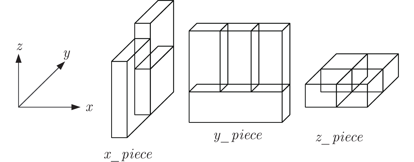
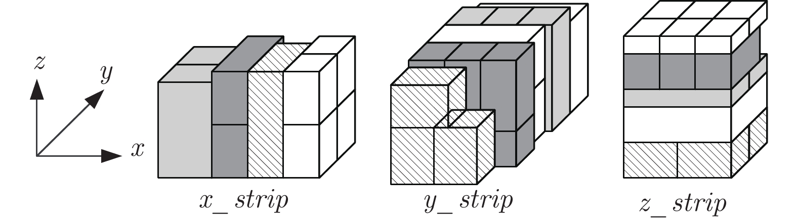
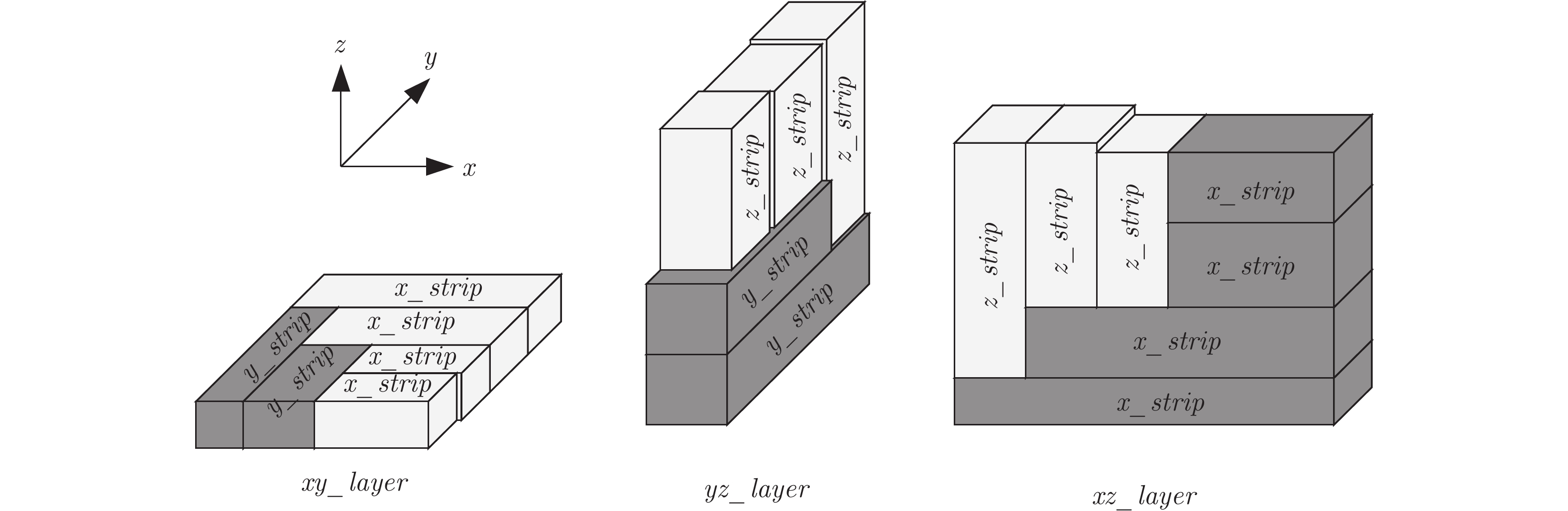
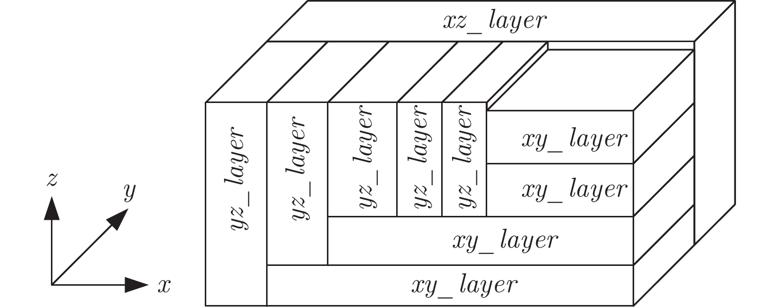
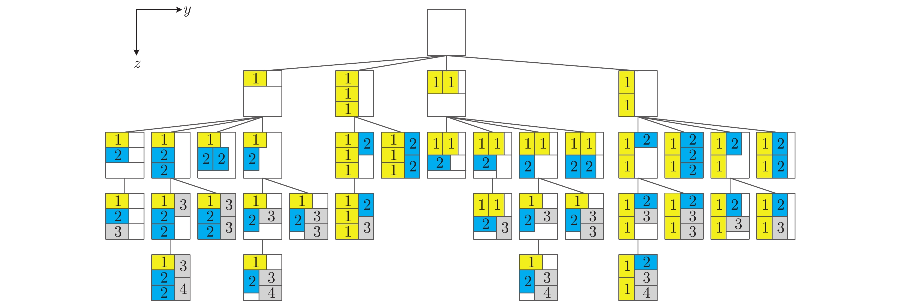
摘要: 提出了一种求解三维装箱问题的多层树搜索算法, 该算法采用箱子–片–条–层–实体的顺序生成装载方案, 装载方案由实体表示. 该算法由3层搜索树构成. 第1层为三叉树, 每个树节点的3个分叉分别对应向实体中填入XY面平行层、XZ面平行层、YZ面平行层; 第2层为二叉树, 每个树节点的两个分叉分别对应向层内装载两个相互垂直的最优条; 第3层为四叉树, 用于将同种的多个箱子生成片. 在同时满足摆放方向约束和完全支撑约束的前提下, 该算法求解BR12~BR15得到的填充率高于现有装箱算法.Abstract: This paper presents a multiple-level tree search algorithm for the three dimensional container loading problem. This algorithm generates a loading plan in the box-piece-strip-layer-entity sequence. Hereby an entity denotes a loading plan. This algorithm consists of three levels of search tree. The first level is a ternary tree. In this tree the three branches of each node correspond to filling three layers which are parallel to the XY-plane, the XZ-plane, and the YZ-plane, respectively. The second level is a binary tree. In this tree the two branches of each node correspond to loading two orthogonal strips into a layer, respectively. The third level is a quad tree to search the best piece. In this tree the boxes of the same kind are integrated into a piece. The proposed algorithm achieves better filling rate for BR12~BR15 than the existing algorithms when the orientation constraint and the full-support constraint are satisfied.
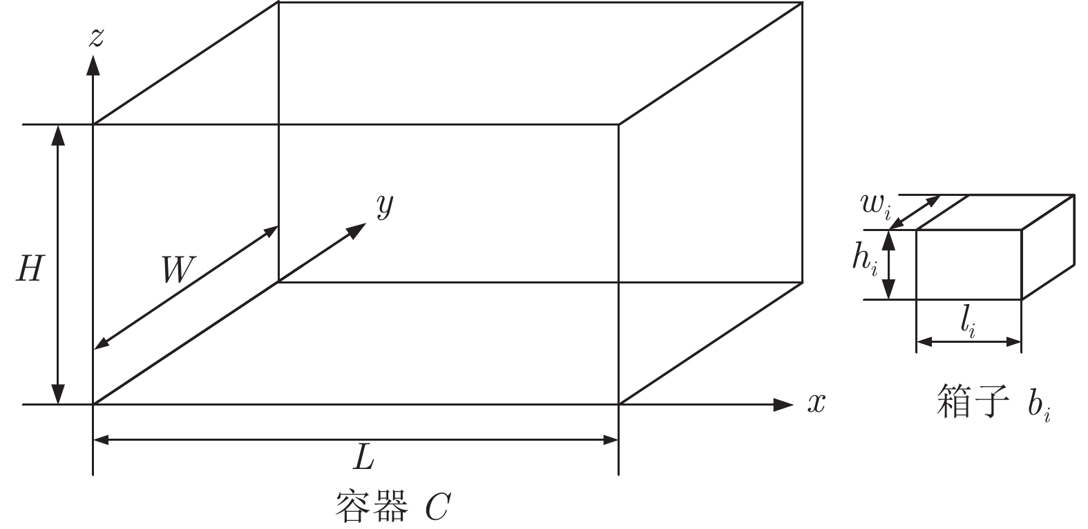
-
时间序列数据在现实生活中广泛存在, 例如金融领域中的交易数据和经济统计数据、消费电商领域中的用户浏览和购买数据、医疗领域中的医疗器械的信号记录、天气监测站记录的天气指标数据等[1-4]. 这些时间序列数据是相应领域非常宝贵的数据资源, 对这些数据的准确、有效分析和利用有助于减小人力成本, 提高生产效率, 提高经济收益[5].
现实中的时间序列通常具有复杂的非线性动态, 这为时间序列预测带来了困难. 另外, 由于人类活动或自然运动的影响, 时间序列数据常常体现出一定的周期性. 周期性的提取对时间序列预测有着积极意义. 时间序列的趋势同样具有重要的意义, 有时甚至作为预测的目的.
传统的时间序列分析方法源自于自回归模型(Autoregressive model, AR)和移动平滑模型(Mo-ving average, MA). 自回归移动平滑模型(Autoregressive model and moving average, ARMA)和在其基础上发展起来的自回归差分移动平滑模型(Auto-regressive integrated moving average, ARIMA)是时间序列分析的经典方法[6]. 另外, 自回归条件异方差模型(Autoregressive conditional heteroscedasticity, ARCH)[7]和广义自回归条件异方差模型(Gen-eralized autoregressive conditional heteroscedasticity, GARCH)[8]引入了异方差, 对时间序列的波动性进行建模. 基于机器学习的支持向量机回归(Sup-port vactor regression, SVR)和核岭回归(Kernel ridge regression, KRR)等方法在时间序列分析上已经有大量的研究[9-11]. 随着深度学习理论的发展, 循环神经网络(Recurrent neural networks, RNNs)已经成为处理时间序列数据的主流, 在大量应用场景中取得了不俗的效果[12-13]. 回声状态网络(Echo state network, ESN)也是时间序列预测的常用模型[14].
传统的时间序列分析方法基于平稳性假设[15], 对短期平稳的时间序列有较好的预测效果, 但是难以对复杂非线性时间序列数据进行有效建模. SVR和KRR等机器学习方法使用滑动窗口的方式处理预测序列, 忽略了时间序列数据的序列属性, 不能很好地捕捉时间序列中的长时依赖. 同时SVR和KRR受限于模型容量, 难以达到预测非线性时间序列的最佳效果. 深度神经网络由于其超强的拟合能力, 在复杂非线性时间序列数据的处理方面有着天然的优势. 同样对于分割后的序列窗口, 深度神经网络仍能从中捕捉时间序列的长期依赖.
能源领域是产生大量时间序列的领域, 如电力用量数据、风力序列数据、太阳能数据和电力价格数据等. 其中, 电力价格是能源市场上的关键因素, 影响着能源市场的流通和运行. 能源市场的自由属性使电力价格具备了金融商品性质, 但其还受到电力传输和需求量的影响. 电力传输受电网传输容量的限制, 而电力需求量受人类活动和天气因素的影响. 在这些影响因素下, 电力价格数据呈现出长期复杂非线性动态, 体现出高波动性. 另外电力价格还存在着明显的周期性.
传统的时间序列预测方法对电力价格的预测已有大量研究和应用[16], 而循环神经网络在电力价格预测中同样取得了不错的效果[17]. 针对能源领域时间序列的周期性属性, 传统的方法主要采用信号处理方法, 而常规的循环神经网络中并没有对时间序列的周期性进行建模的模块. 目前, 许多研究针对数据的周期性展开, 主要研究工作有: Clements等[18]提出了多方程时间序列方法, 在方程中加入了周期设定, 对澳洲能源市场的电力负载进行预测; Anbazhagan等[19]使用离散余弦变换处理原始序列, 并用神经网络进行建模; Rafiei等[20]使用小波变换处理原始序列, 并用极限学习机对分解结果进行建模等.
针对循环神经网络难以对时间序列数据的周期性直接进行建模的问题, 本文结合时间序列周期分解的思想, 设计了循环神经网络的周期损失和趋势损失, 分别对时间序列中的周期和趋势进行辅助建模; 在多任务学习框架下, 将周期损失、趋势损失和模型自身的损失函数相结合, 联合优化循环神经网络. 提出的模型用于能源市场的电力价格预测, 实验结果取得了较好的预测精度, 验证了周期和趋势对时间序列预测的作用, 说明本文提出的周期损失和趋势损失能够有效地辅助模型捕捉数据特征.
1. 循环神经网络
循环神经网络是常用的建模时间序列的神经网络模型. 循环神经网络使用基于时间的反向传播算法(Back-propagation through time, BPTT)来训练网络.
1.1 基础循环单元
基础的循环神经网络及其展开形式如图1所示. 其数学形式为
$$ h_t = f\left( {Ux_t +Wh_{t-1} } \right) $$ (1) $$ o_t = g\left( {Vh_t } \right) \quad \quad \quad \quad \;\; $$ (2) 其中,
$ U $ ,$ V $ ,$ W $ 都是网络的参数,$ f $ 和$ g $ 表示激活函数, 可以是ReLU、sigmoid和tanh等非线性函数.$ x_t $ 表示$ t $ 时刻的输入,$ h_t $ 表示$ t $ 时刻网络的隐藏状态,$ o_t $ 表示$ t $ 时刻网络的输出.基础的循环神经网络在训练时会面对梯度爆炸或梯度消失的问题[21].
1.2 长短时记忆网络
为了克服循环神经网络的梯度爆炸和梯度消失问题, Hochreiter等[22]提出了长短时记忆网络(Long short term memory, LSTM). LSTM的内部结构如图2所示.
LSTM的主要思想是引入门控单元和长时记忆单元. 门控单元负责控制长时记忆单元中状态的记忆、修改和遗忘. 同时, LSTM还具有和基础循环神经网络相同的短期记忆单元.
LSTM的数学表示为
$$ f_t = \sigma \left( {W_f \left[ {h_{t-1} ,x_t } \right]+b_f } \right) \quad \quad \!\!\!$$ (3) $$ i_t = \sigma \left( {W_i \left[ {h_{t-1} ,x_t } \right]+b_i } \right) \quad \quad $$ (4) $$ o_t = \sigma \left( {W_o \left[ {h_{t-1} ,x_t } \right]+b_o } \right) \quad \quad \!\!\!$$ (5) $$ \tilde {C}_t = \tanh \left( {W_C \left[ {h_{t-1} ,x_t } \right]+b_C } \right) $$ (6) $$ C_t = i_t \tilde {C}_t +f_t C_{t-1} \quad \quad \quad \quad \quad \!\!\! $$ (7) $$ h_t = o_t \tanh \left( {C_t } \right) \quad \quad \quad \quad \quad\quad $$ (8) 其中,
$ C_t $ 和$ \tilde {C}_t $ 分别表示$ t $ 时刻的长期记忆和短期记忆,$ f_t $ ,$ i_t $ 和$ o_t $ 分别表示LSTM的遗忘门、输入门和输出门在$ t $ 时刻的值.$ \left( {W_f ,b_f } \right) $ ,$ \left( {W_i ,b_i } \right) $ ,$ \left( {W_o ,b_o } \right) $ 和$ \left( {W_C ,b_C } \right) $ 分别表示LSTM的遗忘门、输入门、输出门和长时记忆单元的参数.$ \sigma $ 代表sigmoid函数.$ x_t $ 表示$ t $ 时刻的输入,$ h_t $ 表示$ t $ 时刻隐藏状态的输出.由于引入了门控单元和长时记忆单元, 状态的更新方式从乘性增量更新变为了加性增量更新[23], 从而一定程度上避免了梯度消失问题.
1.3 门控循环单元
门控循环单元(Gate recurrent unit, GRU)[24]是LSTM的一个重要变体. 相比于LSTM, GRU进行了一定的简化: 将遗忘门和输入门合并成为一个门控单元, 称为更新门; 去除了长期记忆单元, 与隐藏状态混合, 保留短期记忆单元; 去除了输出门, 改为重置门. GRU的内部结构如图3所示.
GRU的数学表示为
$$ z_t = \sigma \left( {W_z \left[ {h_{t-1} ,x_t } \right]} \right) \quad \quad \quad $$ (9) $$ r_t = \sigma \left( {W_r \left[ {h_{t-1} ,x_t } \right]} \right) \quad \quad \quad $$ (10) $$ \tilde {h}_t = \tanh \left( {W\left[ {r_t \times h_{t-1} ,x_t } \right]} \right) $$ (11) $$ h_t = \left( {1-z_t } \right)h_{t-1} +z_t \tilde {h}_t \quad \quad $$ (12) 其中,
$ \tilde {h}_t $ 表示$ t $ 时刻的短期记忆,$ h_t $ 表示$ t $ 时刻的隐藏状态.$ z_t $ 和$ r_t $ 分别表示GRU的更新门和重置门在$ t $ 时刻的值.$ W_z $ ,$ W_r $ 和$ W $ 分别表示GRU的更新门、重置门和短期记忆单元的参数.GRU大大精简了参数, 相同隐藏状态的GRU的参数量约为LSTM的2/3, 使得模型更不容易过拟合. 本文使用GRU作为默认的循环神经网络模型.
2. 基于周期损失和趋势损失的时间序列预测
结合时间序列周期分解, 设计了循环神经网络的周期损失和趋势损失, 将周期损失、趋势损失和模型自身的损失函数相结合, 在多任务学习框架下, 联合优化循环神经网络.
2.1 周期分解
周期分解是一种对时间序列的周期和趋势建模的经典方式.
周期建模是指, 针对周期性的时间序列, 可以显式的考虑序列跨周期的关系. 周期性的一种形式化表述为
$$ \begin{split} & ACF\left( {x_t ,x_{t-T} } \right)\gg ACF\left( {x_t ,x_{t-\tau } } \right) \\ & \quad \quad \quad \quad \quad \quad \quad \quad \quad \!\!\!\! \forall \tau :od \left( {\tau ,T} \right)\ne 0 \end{split} $$ (13) 其中,
$ ACF $ 代表自相关函数. 周期序列按照周期的延迟序列的自相关性应该远远大于其他的延迟序列.趋势建模是指除了建模每一个具体时间点的具体数值, 还应该捕捉到一段时间的“整体状态”, 包括总体走势、变化范围等因素.
可以认为, 时间序列是趋势、周期和余差的组合. 时间序列的分解可以是加性的, 也可以是乘性的, 即
$$ X_t = T_t +S_t +R_t $$ (14) $$ X_t = T_t \times S_t \times R_t $$ (15) 其中,
$ X_t $ 表示原始时间序列,$ T_t $ 表示趋势分量,$ S_t $ 表示周期分量,$ R_t $ 表示余差. 乘性的组合可以通过对数函数转换为加性组合, 所以这两种组合实质上是一致的.2.2 周期损失函数和趋势损失函数
时间序列的周期分解启发了周期损失函数和趋势损失函数的提出.
周期损失函数鼓励循环神经网络预测的隐藏状态出现周期性. 假设一个循环神经网络的隐藏状态具有周期性, 它的隐藏状态需要满足一定的条件:
$$ \begin{split} \cos nt =\; & h_t +h_{t+1} +\cdots +h_{t+T-1}\cong \\ & h_{t+1} +h_{t+2} +\cdots +h_{t+T} \end{split} $$ (16) 即有
$$ h_t \cong h_{t+T} $$ (17) 为了在循环神经网中加入这样的隐藏状态关系, 在
$ \left[ {t_1 ,t_2 ,\cdots ,t_n } \right] $ 的时间窗上定义如下的周期损失函数$$ \ell _{\rm seasonal} \left( {kT} \right) = \frac{1}{n}\sum\limits_{t = t_1 }^{t_n } {D\left( {h_t ,h_{t+\tau } } \right)} $$ (18) 其中,
$ D\left( {\ast ,\ast } \right) $ 表示距离度量函数,$ \tau $ 表示隐藏状态之间的时间跨度.针对周期为
$ T $ 的时间序列, 一般取$ \tau = kT $ .$ \tau $ 也可以取1, 这样式(18)可以视为循环神经网络的一种正规化方法.$ D\left( {\cdot ,\cdot } \right) $ 一般取平方距离, 此时的周期损失为$$ \ell _{\rm seasonal} \left( {kT} \right) = \frac{1}{nm}\sum\limits_{t = t_1 }^{t_n } {\sum\limits_{i = 1}^m {\left\| {h_t^{\left( i \right)} -h_{t+kT}^{\left( i \right)} } \right\|^2} } $$ (19) 其中,
$ m $ 表示循环神经网络的隐藏状态的维度,$ h_t^{\left( i \right)} $ 表示$ t $ 时刻隐藏状态的第$ i $ 维的值. 更长周期跨度有助于鼓励长距离的周期平稳性.在很多实际应用中, 每个时间点的数值并不是最受关注的问题, 而关注的重点在于捕获某种趋势. 时间序列的趋势可以由一段时间内的均值、最大最小值和波动率来反映.
在
$ \left[ {t_1 ,t_2 ,\cdots ,t_n } \right] $ 的时间窗上对时间序列的趋势进行建模, 从均值、最大最小值和波动率的角度可以得到如下的几个趋势损失函数$$ \begin{split} \ell _{\rm trend}^{\rm MEAN} \left( w \right) =\; & \frac{1}{n}\sum\limits_{t = t_1 }^{t_n } {\left\| {mean\left( {\hat {y}_{t-w+1} ,\cdots ,\hat {y}_t } \right)} \right.}- \\ & \left. {mean\left( {y_{t-w+1} ,\cdots ,y_t } \right)} \right\|^2 \end{split} $$ (20) $$ \begin{split} \ell _{\rm trend}^{\rm MAX} \left( w \right) =\; & \frac{1}{n}\sum\limits_{t = t_1 }^{t_n } {\left\| {\max \left( {\hat {y}_{t-w+1} ,\cdots ,\hat {y}_t } \right)} \right.} - \\ & \left. {\max \left( {y_{t-w+1} ,\cdots ,y_t } \right)} \right\|^2 \end{split}\;\;\;\; $$ (21) $$ \begin{split} \ell _{\rm trend}^{\rm MIN} \left( w \right) =\; & \frac{1}{n}\sum\limits_{t = t_1 }^{t_n } {\left\| {\min \left( {\hat {y}_{t-w+1} ,\cdots ,\hat {y}_t } \right)} \right.} -\\ &\left. {\min \left( {y_{t-w+1} ,\cdots ,y_t } \right)} \right\|^2 \end{split} $$ (22) $$ \begin{split} \ell _{\rm trend}^{\rm VAR} \left( w \right) =\; & \frac{1}{n}\sum\limits_{t = t_1 }^{t_n } {\left\| {var\left( {\hat {y}_{t-w+1} ,\cdots ,\hat {y}_t } \right)} \right.} - \\ & \left. {var\left( {y_{t-w+1} ,\cdots ,y_t } \right)} \right\|^2 \end{split} $$ (23) 其中,
$ \ell _{\rm trend}^{\rm MEAN} $ 、$ \ell _{\rm trend}^{\rm MAX} $ 、$ \ell _{\rm trend}^{\rm MIN} $ 和$ \ell _{\rm trend}^{\rm VAR} $ 分别代表均值趋势损失、最大趋势损失、最小趋势损失和波动趋势损失.$ w $ 表示趋势窗宽, 一般与序列的时间窗宽度$ n $ 不同.$ \hat {y} $ 是循环神经网络的预测值,$ y $ 是真实值.2.3 基于多任务学习的混合预测模型
在机器学习中, 通常只关注一个优化目标. 多任务学习(Multi-task learning)[25]是同时学习多个相关的任务并在这些任务间共享某些底层的特征表示的机器学习方式. 在深度学习中, 多任务学习非常普遍.
一般地, 针对多个优化目标, 多任务学习框架中存在共同优化和分开交替优化两种优化方式. 共同优化适用于紧密相关的任务, 分开交替优化则适用于不相关任务和对抗性任务. 周期性和趋势约束作为时间序列预测的辅助任务, 与预测任务关系密切. 因此, 将周期损失和趋势损失引入优化目标进行共同优化是合理的.
本文根据多任务学习的框架, 将周期损失和趋势损失将作为预测任务的共同优化目标, 在原来的损失函数的基础上, 加入了辅助损失函数, 得到时间序列多任务学习混合模型的优化目标函数
$$ J = L_{\rm main} +\lambda _S \ell _{\rm seasonal} +\ell _{\rm trend} \quad \quad \quad \;$$ (24) $$ \begin{split} \ell _{\rm trend} =\; & \lambda _T^{\rm MEAN} \ell _{\rm trend}^{\rm MEAN} +\lambda _T^{\rm MAX} \ell _{\rm trend}^{\rm MAX}+ \\ & \lambda _T^{\rm MIN} \ell _{\rm trend}^{\rm MIN} +\lambda _T^{\rm VAR} \ell _{\rm trend}^{\rm VAR} \end{split} \;\;\;\; $$ (25) 其中,
$ \lambda _S $ 是周期损失的权重,$ \lambda _{\rm trend}^{\rm MEAN} $ ,$ \lambda _{\rm trend}^{\rm MAX} $ ,$ \lambda _{\rm trend}^{\rm MIN} $ 和$ \lambda _{\rm trend}^{\rm VAR} $ 分别代表对应的趋势损失的权重.引入周期损失和趋势损失的循环神经网络依然可以通过BPTT算法来训练.
3. 仿真实验
3.1 能源市场简介
欧洲能源交易所(European Power Exchange, EPEX)是欧洲最重要的能源交易市场, 覆盖了德国、法国、英国等欧洲最主要的国家. 电力在各个国家的电网之间进行交换, 其中一部分是通过事先规划的方式, 而另一部分则通过能源交易所进行交易. 每个国家都会有自己的子市场, 例如EPEX法国市场. EPEX 法国市场的现货市场主要分为三个子市场: 日前交易市场(Day-ahead market)、日内交易市场(Intraday market)和再平衡市场(Balancing market). 能源市场的实际交易主要发生在日前交易市场. 通常EPEX法国市场的日前交易市场每天形成24个报价, 即每小时一个报价.
图4展示了EPEX法国市场2012年~2015年的一天的不同小时的价格的均值和标准差. 可以看出, 电力价格的标准差非常高, 在均值的1/4以上, 在个别时间段(9:00~11:00)的标准差甚至超出了均值. 这说明EPEX法国市场的电力价格具有超高的波动性. 图5和图6分别展示了EPEX法国市场2012年~2015年每年的日级别平均价格和周级别平均价格. 可以看出, 无论是按日的级别还是周的级别对电价进行统计, 每年的电力价格均呈现非常相似的走势, 体现出明显的周期性.
3.2 实验及结果
选用EPEX法国市场的电力价格数据作为仿真来源. 数据来自日前电力市场, 时间段取自2012年1月1日~2016年6月30日, 其中2012年1月1日~2015年12月31日(共1 461天)的序列数据用来做训练和验证, 2016年1月1日~2016年6月30日(共182天)的序列数据用来做测试. 通常每天有24个时间点(夏令时转换日有23个时间点, 冬令时转换日有25个时间点).
为了保证数据的稳定性, 需要对数据进行预处理, 去除数据的均值和波动率的影响
$$ \tilde {x}_t^h = \frac{x_t^h -\bar {x}_t }{std\left( x \right)} $$ (26) 其中,
$ x $ 代表所有的序列数据,$ h $ 表示序列中的年份信息(2012年~2016年),$ x_t^h $ 表示不同年份的在同一时间点$ t $ 的序列值,$ \bar {x}_t $ 表示$ x_t^h $ 按年份展开的子序列的均值,$ \tilde {x}_t^h $ 为处理后的序列值. 经过这样的变换, 大部分时间点的数据处于[−1, 1]区间, 可以避免出现一些数值问题.实验对比了几种基础的循环神经网络: RNN、LSTM和GRU. 为了分析周期损失和趋势损失的作用, 在GRU的基础上分别添加周期损失、趋势损失或者两者都添加.
循环神经网络需要调整的超参数有: 隐层大小、优化器、初始学习率、批大小(batch size)、训练轮数(epochs)以及延迟窗宽. 针对引入周期损失和趋势损失的GRU, 还需要调整的有: 周期损失系数
$ \lambda _S $ 、周期损失中的周期跨度kT、趋势损失系数($ \lambda _{\rm trend}^{\rm VAR} $ 、$ \lambda _{\rm trend}^{\rm MEAN} $ 、$ \lambda _{\rm trend}^{\rm MAX} $ 和$ \lambda _{\rm trend}^{\rm MIN} $ )和趋势窗宽$ w $ . 这里考虑能源市场的短期周期, 故$ k $ 取1,$ T $ 取24. 由于能源市场的价格预测任务往往不关注每日的平均价格和价格的波动预测的误差,$ \lambda _{\rm trend}^{\rm MEAN} $ 和$ \lambda _{\rm trend}^{\rm VAR} $ 的值都预设为0, 不再纳入超参数选择中. 能源市场的价格预测比较关注一天内的最大最小值, 因此趋势窗宽$ w $ 设为24. 训练时间段的最后一个月(2015年12月)作为验证时间段. 通过在验证时间段内进行多次实验的方式来选取超参数. 选出来的超参数将被用于在完整的训练时间段上的训练. 循环神经网络的超参数设置如表1所示.表 1 循环神经网络的超参数设置Table 1 The hyperparameters of RNN超参数 具体取值 隐层大小 64 优化器 RMSProp, 配合梯度裁剪 初始学习率 0.001 批大小 64 训练轮数 12 延迟窗宽 14 表2列出了周期损失和趋势损失的合理的取值范围.
表 2 周期损失和趋势损失的权重范围Table 2 Weights range of seasonal loss and trend loss权重 取值范围 $\lambda_S $ 0.05~0.15 $\lambda_T^{\rm{MEAN}} $ 0 $\lambda_T^{\rm{MAX}} $ 0.05~0.1 $\lambda_T^{\rm{MIN}} $ 0.05~0.1 $\lambda_T^{\rm{VAR}} $ 0 除了与基础的循环神经网络进行对比, 另外还选取了ARIMA、SVR和KRR作为对比模型. SVR和KRR的超参数均通过在训练时间段内的5折交叉验证直接选取, 均选用3阶多项式核. 为了满足ARIMA模型的静态性要求, 电力价格数据还需要经过特殊处理, 即将序列减去最小值后取对数, 然后进行天级和周级的延迟差分
$$ {p}' = (1-\beta ^{24})(1-\beta ^{168})\ln (p-\min p+1) $$ (27) 实验采用均方根误差(Root mean square error, RMSE)和平均绝对误差(Mean absolute error, MAE)作为评价指标
$$ RMSE = \sqrt {\frac{1}{N}\sum\limits_{t = 1}^N {\left( {\hat {y}_t -y_t } \right)^2} } $$ (28) $$ MAE = \frac{1}{N}\sum\limits_{t = 1}^N {\left| {\hat {y}_t -y_t } \right|} \quad \quad \quad $$ (29) 其中,
$ N $ 表示测试时间段的时间点数. RMSE也是各模型训练时的损失指标.为了更合理地比较趋势损失的影响, 本文还引入了两个额外指标, 最大趋势绝对误差
$ {MAE}^{\rm{MAX}} $ 和最小趋势绝对误差$ {MAE}^{\rm{MIN}} $ , 分别考察模型对每天电力价格最大值和最小值的预测能力$$ \begin{split} MAE^{\rm{MAX}} =\; & \frac{1}{M}\sum\limits_{t = 1}^M {\left| {\max \left( {\hat {y}_{t-w+1} ,\cdots ,\hat {y}_t } \right)} \right.}- \\ & \left. {\max \left( {y_{t-w+1} ,\cdots ,y_t } \right)} \right| \\ \end{split} $$ (30) $$ \begin{split} MAE^{\rm{MIN}} =\; & \frac{1}{M}\sum\limits_{t = 1}^M {\left| {\min \left( {\hat {y}_{t-w+1} ,\cdots ,\hat {y}_t } \right)} \right.}- \\ & \left. {\min \left( {y_{t-w+1} ,\cdots ,y_t } \right)} \right| \\ \end{split} $$ (31) 其中,
$ M $ 表示测试时间段划分的趋势窗的数目.由于神经网络在训练过程中具有一定的随机性, 每次训练的得到的结果都有所不同. 为了保证实验结果的可信性, 对所有循环神经网络采用了重复10次训练并取测试结果的平均值和标准差. 各方法在能源价格预测的结果见表3.
表 3 各种方法的能源价格预测效果对比Table 3 The result comparisons of different methods for electricity price forecasting模型 RMSE MAE ${MAE}^{\rm{MAX}}$ ${MAE}^{\rm{MIN}}$ ARIMA 6.41 4.77 5.15 4.82 SVR 4.91 3.71 4.27 3.34 KRR 5.14 3.75 3.81 3.78 RNN 5.09±0.24 3.75±0.19 3.72±0.28 3.78±0.19 LSTM 4.90±0.18 3.65±0.17 3.65±0.42 3.61±0.26 GRU 4.83±0.19 3.54±0.06 3.64±0.31 3.56±0.26 GRU, $\lambda_S$ = 0.1, $\lambda_T^{\rm{MAX}}$ = 0, $\lambda_T^{\rm{MIN}}$ = 0 4.71±0.16 3.49±0.13 3.53±0.28 3.53±0.15 GRU, $\lambda_S$ = 0.05, $\lambda_T^{\rm{MAX}}$ = 0, $\lambda_T^{\rm{MIN}}$ = 0 4.74±0.11 3.45±0.18 3.53±0.23 3.48±0.26 GRU, $\lambda_S$ = 0 , $\lambda_T^{\rm{MAX}}$ = 0.1 , $\lambda_T^{\rm{MIN}}$ = 0.1 4.85±0.16 3.57±0.20 3.41±0.26 3.41±0.18 GRU, $\lambda_S$ = 0 , $\lambda_T^{\rm{MAX}}$ = 0.05 , $\lambda_T^{\rm{MIN}}$ = 0.05 4.83±0.11 3.54±0.08 3.39±0.18 3.42±0.15 GRU, $\lambda_S$ = 0.1, $\lambda_T^{\rm{MAX}}$ = 0.1 , $\lambda_T^{\rm{MIN}}$ = 0.1 4.68±0.08 3.45±0.03 3.35±0.13 3.33±0.12 GRU, $\lambda_S$ = 0.05, $\lambda_T^{\rm{MAX}}$ = 0.05 , $\lambda_T^{\rm{MIN}}$ = 0.05 4.60±0.15 3.34±0.12 3.38±0.13 3.27±0.11 从实验结果可以看出, 对于电力价格预测这类复杂的时间序列预测问题, ARIMA模型的预测效果不佳, SVR、KRR和RNN的效果接近且远远优于ARIMA模型LSTM和GRU的预测效果比SVR和KRR更好, 而基础的GRU在对比模型中效果最佳. 添加周期损失能对GRU起到比较好的辅助效果, 有助于降低模型的预测误差, 提升预测效果. 趋势损失最直接的影响是显著降低最大趋势误差和最小趋势误差, 说明模型通过趋势损失捕捉到了数据在时间窗内的趋势信息(包括电力价格的极值、均值和变化率等), 这对模型捕捉数据特征的能力起到了有力的补充. 另外可以注意到的是, 加入周期损失也能够降低最大趋势误差和最小趋势误差. 这说明周期损失有助于网络捕捉一些数据的本质特征. 实验结果表明: 同时引入周期损失和趋势损失可以使GRU的性能达到最佳.
引入周期损失和趋势损失的GRU在最佳的参数下(
$ \lambda _S = \lambda _T^{\rm{MAX}} = \lambda _T^{\rm{MIN}} = 0.05 $ )的预测结果如图7所示.可以看出, 引入周期损失和趋势损失的GRU对电力价格数据的预测效果不错, 预测曲线对真实数值的走势和变化跟踪准确. 预测曲线具有非常好的周期性, 这体现了周期损失中周期性约束的作用. 同时, 预测曲线更偏向于平稳的预测, 这在一定程度上避免了噪声带来的预测性能损失. 另外, 预测曲线在正常情况下的最大最小值的预测效果很好, 说明趋势损失能够起到有效的监督效果. 但可以观察到的是, 模型在一些极端值(电力价格的异常攀升和下降)上的预测效果不佳. 这涉及到突变的预测问题, 在现有模型框架下难有较好的预测效果.
为了进一步分析周期损失的效果, 将GRU和加入周期损失的GRU在训练一段时间之后的隐藏状态
$ h_t $ 分别抽出, 并将向量$ h_t $ 的均值作对比, 部分结果如图8所示.由于时间序列本身具有一定的周期性, 使得隐藏状态序列都表现出了一定的周期性. 但是, 使用了周期损失的GRU的隐藏状态明显更加平稳, 并且每个周期内的数值更加平滑; 而未使用周期损失的GRU的隐藏状态的波动性更大, 并且单个周期内的波动也更大. 这些更大的波动可以认为是捕捉到了更多的噪声. 所以, 周期损失有助于捕捉数据更本质的特征而非噪声.
4. 结论
循环神经网络能够提取时间序列中的深层信息, 是非常有效的时间序列预测方法. 本文通过定义周期损失和趋势损失的合理形式, 试图在循环神经网络内对时间序列的周期和趋势进行建模, 改善模型的性能, 建立了基于周期性建模和多任务学习的时间序列预测模型. 在能源市场价格预测的任务的仿真实验表明: 本文提出的周期损失能够有效引导循环神经网络学习数据的周期性, 提升预测效果, 降低数据噪声的影响. 周期损失还有助于模型捕捉数据的本质特征. 趋势损失则能对提升趋势相关的预测任务的预测效果.
-
表 1 各种算法对BR1~BR7的填充率比较
Table 1 Comparison of filling rates of BR1~BR7 by various algorithms
算法 约束 填充率 (%) BR1 BR2 BR3 BR4 BR5 BR6 BR7 平均 GA_GB[16] C1&C2 85.80 87.26 88.10 88.04 87.86 87.85 87.68 87.5 GRASP[23] C1 93.52 93.77 93.58 93.05 92.34 91.72 90.55 92.65 FDA[11] C1 92.92 93.93 93.71 93.68 93.73 93.63 93.14 93.53 HSA[21] C1&C2 93.81 93.94 93.86 93.57 93.22 92.72 91.99 93.30 Maximal-space[24] C1 93.85 94.22 94.25 94.09 93.87 93.52 92.94 93.82 A2[12] C1 − − − − − − − − CLTRS[7] C1 95.05 95.43 95.47 95.18 95.00 94.79 94.24 95.02 C1&C2 94.51 94.73 94.74 94.41 94.13 93.85 93.20 94.22 MLHS[31] C1 94.92 95.48 95.69 95.53 95.44 95.38 94.95 95.34 C1&C2 94.49 94.89 95.20 94.94 94.78 94.55 93.95 94.69 MLTrS C1 93.81 93.83 93.80 93.98 93.97 93.83 93.91 93.88 C1&C2 93.48 93.41 93.79 93.85 93.43 93.65 93.63 93.61 表 2 各种算法对BR8~BR15的填充率比较
Table 2 Comparison of filling rates of BR8~BR15 by various algorithms
算法 约束 填充率 (%) BR8 BR9 BR10 BR11 BR12 BR13 BR14 BR15 平均 GA_GB[15] C1&C2 87.52 86.46 85.53 84.82 84.25 83.67 82.99 82.47 84.71 GRASP[23] C1 90.26 89.50 88.73 87.87 87.18 86.70 85.81 85.48 87.69 FDA[11] C1 92.92 92.49 92.24 91.91 91.83 91.56 91.30 91.02 91.9 HSA[21] C1&C2 90.56 89.7 89.06 88.18 87.73 86.97 86.16 85.44 87.98 Maximal-space[24] C1 91.02 90.46 89.87 89.36 89.03 88.56 88.46 88.36 89.39 A2[12] C1 88.41 88.14 87.9 87.88 87.92 87.92 87.82 87.73 87.97 CLTRS[7] C1 93.70 93.44 93.09 92.81 92.73 92.46 92.40 92.40 92.88 C1&C2 92.26 91.48 90.86 90.11 89.51 88.98 88.26 87.57 89.88 MLHS[31] C1 94.54 94.14 93.95 93.61 93.38 93.14 93.06 92.90 93.59 C1&C2 93.12 92.48 91.83 91.23 90.59 89.99 89.34 88.54 90.89 MLTrS C1 93.98 93.97 93.78 93.75 93.63 93.43 93.25 93.12 93.61 C1&C2 91.82 91.69 91.55 91.24 91.21 91.03 90.78 90.59 91.24 -
[1] Dyckhoff H, Finke U. Cutting and Packing in Production and Distribution. Heidelberg: Physica-Verlag, 1992 [2] George J A, Robinson D F. A heuristic for packing boxes into a container. Computers and Operations Research, 1980, 7(3): 147−156 doi: 10.1016/0305-0548(80)90001-5 [3] Dyckhoff, H. A typology of cutting and packing problems. European Journal of Operational Research, 1990, 44(2): 145−159 doi: 10.1016/0377-2217(90)90350-K [4] Wäscher G, Haußner H, Schumann H. An improved typology of cutting and packing problems. European Journal of Operational Research, 2007, 183(3): 1109−1130 doi: 10.1016/j.ejor.2005.12.047 [5] Bortfeldt A, Wäscher G. Constraints in container loading — a state-of-the-art review. European Journal of Operational Research, 2013, 229(1): 1−20 doi: 10.1016/j.ejor.2012.12.006 [6] Scheithauer G. Algorithms for the container loading problem. In: Proceedings of the 1991 on Operations Research. Berlin, Heidelberg, Germany: Springer, 1992. 445−452 [7] Fanslau T, Bortfeldt A. A tree search algorithm for solving the container loading problem. INFORMS Journal on Computing, 2010, 22(2): 222−235 doi: 10.1287/ijoc.1090.0338 [8] Fekete S P, Schepers J, Van der Veen J C. An exact algorithm for higher-dimensional orthogonal packing. Operations Research, 2007, 55(3): 569−587 doi: 10.1287/opre.1060.0369 [9] Bischoff E E, Ratcliff B S W. Issues in the development of approaches to container loading. Omega, 1995, 23(4): 377−390 doi: 10.1016/0305-0483(95)00015-G [10] Bischoff E E, Janetz F, Ratcliff M S W. Loading pallets with non-identical items. European Journal of Operational Research, 1995, 84(3): 681−692 doi: 10.1016/0377-2217(95)00031-K [11] He K, Huang W Q. An efficient placement heuristic for three-dimensional rectangular packing. Computers and Operations Research, 2011, 38(1): 227−233 [12] Huang W Q, He K. A caving degree approach for the single container loading problem. European Journal of Operational Research, 2009, 196(7): 93−101 [13] He K, Huang W Q. A caving degree based flake arrangement approach for the container loading problem. Computers and Industrial Engineering, 2010, 59(2): 344−351 [14] Lim A, Rodrigues B, Wang Y. A multi-faced buildup algorithm for three-dimensional packing problems. Omega, 2003, 31(6): 471−481 doi: 10.1016/j.omega.2003.08.004 [15] 张德富, 魏丽军, 陈青山, 陈火旺. 三维装箱问题的组合启发式算法. 软件学报, 2007, 18(9): 2083−2089 doi: 10.1360/jos182083Zhang De-Fu, Wei Li-Jun, Chen Qing-Shan, Chen Huo-Wang. A combinational heuristic algorithm for the three dimensional packing problem. Journal of Software, 2007, 18(9): 2083−2089 doi: 10.1360/jos182083 [16] Gehring H, Bortfeldt A. A genetic algorithm for solving the container loading problem. International Transactions in Operational Research, 1997, 4(5–6): 401−418 doi: 10.1111/j.1475-3995.1997.tb00095.x [17] Bortfeldt A, Gehring H. A hybrid genetic algorithm for the container loading problem. European Journal of Operational Research, 2001, 131(1): 143−161 doi: 10.1016/S0377-2217(00)00055-2 [18] Sixt M. Dreidimensionale Packprobleme. Losungsverfahren Basierend auf den Meta-Heuristiken Simulated Annealing und Tabu-Suche. Frankfurt am Main: Europaischer Verlag der Wissenschaften, 1996. [19] Bortfeldt A, Gehring H, Mack D. A parallel tabu search algorithm for solving the container loading problem. Parallel Computing, 2003, 29(5): 641−662 doi: 10.1016/S0167-8191(03)00047-4 [20] Mack D, Bortfeldt A, Gehring H. A parallel hybrid local search algorithm for the container loading problem. International Transactions in Operational Research, 2004, 11(5): 511−533 doi: 10.1111/j.1475-3995.2004.00474.x [21] 张德富, 彭煜, 朱文兴, 陈火旺. 求解三维装箱问题的混合模拟退火算法. 计算机学报, 2009, 32(11): 2147−2156Zhang De-Fu, Peng Yu, Zhu Wen-Xing, Chen Huo-Wang. A hybrid simulated annealing algorithm for the three-dimensional packing problem. Chinese Journal of Computers, 2009, 32(11): 2147−2156 [22] Bischoff E E. Three-dimensional packing of items with limited load bearing strength. European Journal of Operational Research, 2006, 168(3): 952−966 doi: 10.1016/j.ejor.2004.04.037 [23] Moura A, Oliveira J F. A GRASP approach to the container-loading problem. IEEE Intelligent Systems, 2005, 20(4): 50−57 doi: 10.1109/MIS.2005.57 [24] Parreno F, Alvarez-Valdes R, Oliveira J F, Tamarit J M. A maximal-space algorithm for the container loading problem. INFORMS Journal on Computing, 2007, 20(3): 412−422 [25] Morabito R, Arenales M. An AND/OR-graph approach to the container loading problem. International Transactions in Operational Research, 1994, 1(1): 59−73 [26] Terno J, Scheithauer G, Sommerweiß U, Riehme J. An efficient approach for the multi-pallet loading problem. European Journal of Operational Research, 2000, 123(2): 372−381 doi: 10.1016/S0377-2217(99)00263-5 [27] Eley M. Solving container loading problems by block arrangement. European Journal of Operational Research, 2002, 141(2): 393−409 doi: 10.1016/S0377-2217(02)00133-9 [28] Hifi, M. Approximate algorithms for the container loading problem. International Transactions in Operational Research, 2002, 9(6): 747−774 doi: 10.1111/1475-3995.00386 [29] Pisinger D. Heuristics for the container loading problem. European Journal of Operational Research, 2002, 141(2): 143−153 [30] Lim A, Ma H, Xu J, Zhang X W. An iterated construction approach with dynamic prioritization for solving the container loading problems. Expert Systems with Applications, 2012, 39(4): 4292−4305 doi: 10.1016/j.eswa.2011.09.103 [31] 张德富, 彭煜, 张丽丽. 求解三维装箱问题的多层启发式搜索算法. 计算机学报, 2012, 35(12): 2553−2561 doi: 10.3724/SP.J.1016.2012.02553Zhang De-Fu, Peng Yu, Zhang Li-Li. A multi-layer heuristic search algorithm three dimensional container loading problem. Chinese Journal of Computers, 2012, 35(12): 2553−2561 doi: 10.3724/SP.J.1016.2012.02553 [32] Liu S, Tan W, Xu Z Y, Liu X W. A tree search algorithm for the container loading problem. Computers and Industrial Engineering, 2014, 75: 20−30 [33] 刘胜, 朱凤华, 吕宜生, 李元涛. 求解三维装箱问题的启发式正交二叉树搜索算法. 计算机学报, 2015, 38(8): 1530−1543 doi: 10.11897/SP.J.1016.2015.01530Liu Sheng, Zhu Feng-Hua, Lv Yi-Sheng, Li Yuan-Tao. A heuristic orthogonal binary tree search algorithm for three dimensional container loading problem. Chinese Journal of Computers, 2015, 38(8): 1530−1543 doi: 10.11897/SP.J.1016.2015.01530 [34] Ren J D, Tian Y J, Sawaragi T. A tree search method for the container loading problem with shipment priority. European Journal of Operational Research, 2011, 214(3): 526−535 doi: 10.1016/j.ejor.2011.04.025 [35] Wang N, Lim A, Zhu W B. A multi-round partial beam search approach for the single container loading problem with shipment priority. International Journal of Production Economics, 2013, 145(2): 531−540 doi: 10.1016/j.ijpe.2013.04.028 [36] Lim A, Ma H, Qiu C Y, Zhu W B. The single container loading problem with axle weight constraints. International Journal of Production Economics, 2013, 144(1): 358−369 doi: 10.1016/j.ijpe.2013.03.001 [37] Liu S, Shang X Q, Cheng C J, Zhao H X, Wang F-Y. Heuristic algorithm for the container loading problem with multiple constraints. Computers and Industrial Engineering, 2017, 108: 149−164 [38] Wang L, Lu J W. A memetic algorithm with competition for the capacitated green vehicle routing problem. IEEE/CAA Journal of Automatica Sinica, 2019, 6(2): 516−526 [39] Shang X Q, Shen D Y, Wang F-Y, Nyberg T R. A heuristic algorithm for the fabric spreading and cutting problem in apparel factories. IEEE/CAA Journal of Automatica Sinica, 2019, 6(4): 961−968 [40] Luo C, Shen Z, Evangelou S, Xiong G, Wang F-Y. The combination of two control strategies for series hybrid electric vehicles. IEEE/CAA Journal of Automatica Sinica, 2019, 6(2): 596−608 [41] Shen Z, Shang X Q, Dong X S, Xiong G, Wang F-Y. A learning based framework for error compensation in 3D printing. IEEE Transactions on Cybernetics, 2019, 49(11): 4042−4050 期刊类型引用(2)
1. 卢弘,王耀南,乔非,方遒. 面向可持续生产中多任务调度的双重增强模因算法. 自动化学报. 2024(04): 731-744 . 本站查看
2. 李瑞,龚文引. 改进的基于分解的多目标进化算法求解双目标模糊柔性作业车间调度问题. 控制理论与应用. 2022(01): 31-40 . 百度学术
其他类型引用(13)
-