

-
摘要:
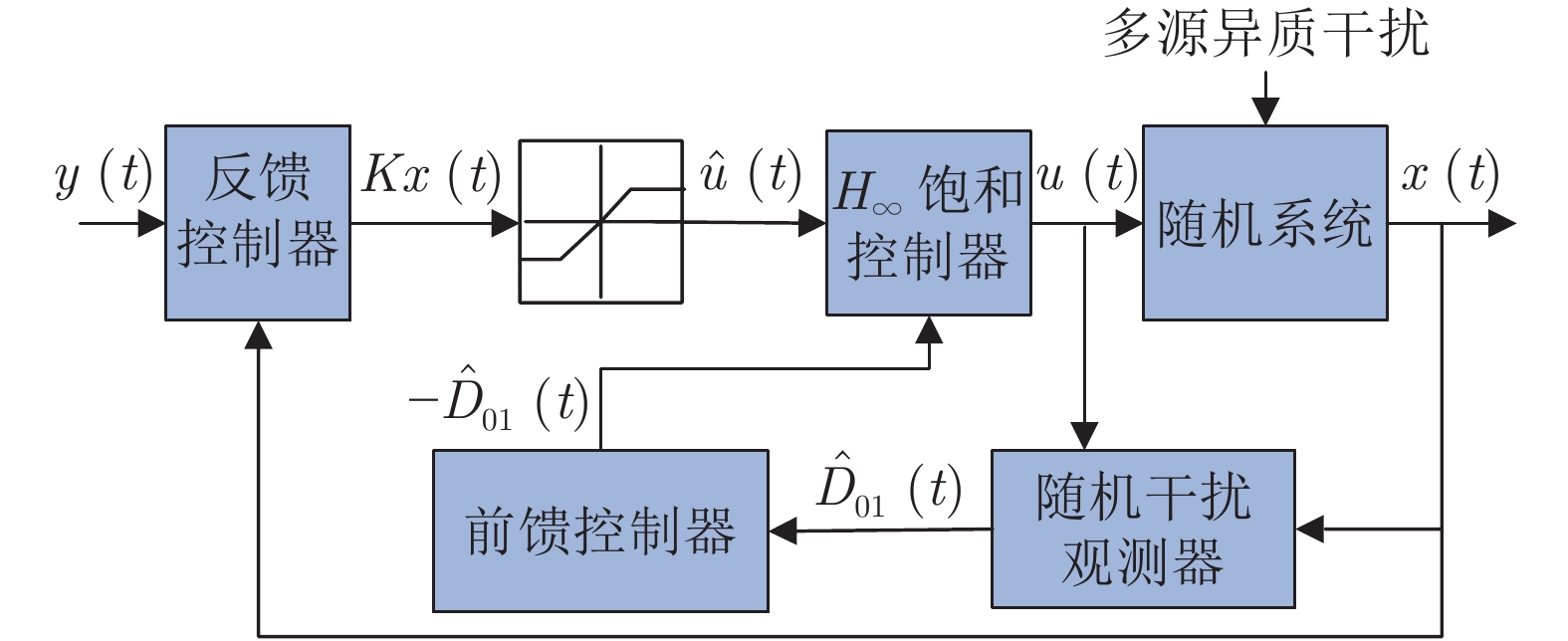
针对一类带有多源异质干扰和输入饱和的随机系统, 研究了其精细抗干扰控制问题. 系统中的多源异质干扰同时包含白噪声,
\begin{document}$H_{2}$\end{document} 范数有界干扰以及外源系统生成的带有状态与干扰耦合的部分信息已知干扰. 针对部分信息已知的干扰, 构建随机干扰观测器对其进行估计. 基于干扰估计, 结合
$H_{\infty}$ 控制方法, 提出基于干扰观测器的精细抗干扰控制策略, 从而实现高精度抗干扰控制. 最后, 仿真结果验证了所提策略的正确性与有效性.
Abstract:The problem of elegant anti-disturbance control are discussed for a class of stochastic systems with multiple heterogeneous disturbances and input saturation. The multiple heterogeneous disturbances simultaneously include white noise,
\begin{document}$H_{2}$\end{document} -norm bounded disturbance and the disturbance with partially-known information which with the coupling of the disturbance and state. To estimate the disturbance with partially-known information, a stochastic disturbance observer (SDO) is constructed. Based on the SDO, a disturbance observer-based elegant anti-disturbance control scheme is proposed by combining disturbance observer based control (DOBC) with
$H_{\infty}$ control, such that higher control accuracy can be achieved. Finally, a simulation example is given to illustrate the effectiveness of the proposed method.
-
随着计算机技术、自动化技术、网络技术的迅猛发展, 现代生产过程的自动控制水平不断提高, 使得进行过程监视与故障诊断, 提升过程的安全性与可靠性, 保证过程稳定与产品的质量成为可能.生产过程发生故障轻则造成产品质量不合格、资源浪费等后果, 重则引起火灾、爆炸等危害人员安全和影响社会安定的恶性事件[1].实际工业生产过程中, 生产负荷、产品特性、原料组分等因素的改变会导致生产工况发生变化, 产生多工况过程.多工况过程的数据具有非高斯、非线性、多模态、中心漂移等特征, 各工况中心不同, 其变量至少有一个是多峰分布, 因此多工况过程的故障检测技术更加复杂且对于保证过程稳定与安全具有重要意义.
针对多工况过程, 常用的两种研究方法[2]为:多模型法和全局模型法.多模型法利用各工况数据建立多个局部模型, 通过多次建模将局部单工况过程扩展成为多工况过程.该方法首要问题即为如何将数据分离成不同子集对应的多个工况.如许仙珍等[3]对传统主成分分析(Principle component analysis, PCA)不能有效解决多工况问题的缺点进行了改进, 提出了一种基于PCA混合模型的多工况过程故障监测方法, 该方法的优点在于能自动获取工况数目, 无需过程先验知识.熊伟丽等[4]针对不同稳态工况之间的过渡过程提出了一种基于多工况识别的过程监测方法, 利用独立主成分分析(Independent component analysis, ICA)和PCA提取各阶段数据的信息. Ge等[5]针对多工况间歇过程提出了一种新的基于贝叶斯推理的过程监测方法, 该方法采用ICA-PCA提取数据特征, 利用支持向量数据描述(Support vector data description, SVDD)方法进行故障检测, 构造超球体, 以超球体的半径作为控制限. Zhao等[6]提出了一种能够同时解决多工况多阶段问题的故障监视方法.孙贤昌等[7]提出了一种基于高斯混合模型(Gaussian mixture models, GMM)的多工况过程故障诊断方法, 该方法使用GMM方法对数据进行聚类分析, 得到工况数和不同工况的分布参数, 而后采用PCA方法建模进行故障检测.多模型法的优点在于步骤分明、监控结果易于解释, 故障识别和诊断相对容易, 但在实际应用中存在依赖过程知识、在线识别工况、模型集优化和模型切换策略等问题.
全局模型法直接从具有多工况特性的历史数据中学习全局模型, 构建表征各工况特性的统一检测指标, 可以避免多模型法存在的问题.郭红杰等[8]提出了一种基于局部近邻标准化策略的故障检测方法, 该方法运用局部近邻标准化策略对数据进行预处理, 消除数据的多工况特性.王国柱等[9]提出了一种加权KNN (K-nearest neighbor, KNN)重构的故障诊断方法, 文中采用KNN规则进行故障检测, 基于KNN的故障检测方法是以距离为衡量, 将数据的非高斯、非线性、多工况的特点随着建模数据直接包含在所建的模型中. Ge等[10]将SVDD方法应用于多工况过程, 通过在特征空间构造一个最小超球体将故障数据与正常数据区分.钟娜等[11]提出了一种基于局部熵成分分析(Local entropy component analysis, LECA)的故障检测方法, 通过KNN-Parzen窗方法估计变量的局部概率密度, 利用信息熵理论挖掘局部信息熵, 最后采用ICA方法建模进行故障检测.针对多模态问题, Ning等[12]提出了基于标签一致性字典学习算法(Label consistent dictionary learning, LCDL)和稀疏贡献图的过程故障诊断方法, 该方法通过标签一致性K-SVD方法从正常历史数据中得到字典, 加入一个单位矩阵扩展字典, 运用扩展字典对检测样本进行稀疏编码, 最后以重构误差作为统计量进行在线监控, 该方法对字典进行扩展, 增加了数据的复杂度和计算量, 而且以重构误差作为统计量的误报率偏高.
本文针对多工况过程, 提出一种在稀疏残差空间构建$k$近邻距离统计量的故障检测方法.将多工况正常数据混合在一起标准化用于建立全局模型, 避免工况识别的工作; 采用稀疏编码方法提取分布散、特征不够集中的多工况数据的字典和稀疏编码, 保持工况特征的同时突出数据特征; 采用多工况正常数据的近似值和原始值的偏差构建新的样本空间-稀}疏残差空间, 提出在稀疏残差空间引入距离统计量作为故障检测指标, 通过稀疏残差空间数据间$k$近邻距离大小衡量数据的相似性, 兼得$k$近邻算法解决非高斯、非线性、多工况问题的优点, 改善多工况过程故障检测效果.
1. 基于稀疏残差距离的故障检测方法
1.1 稀疏残差距离(SRD)的构建
本文提出在稀疏残差空间引入距离统计量, 简称SRD (Sparse residual distance), 具体构建内容如下:
定义多工况正常数据矩阵$X\in {\bf R}^{n\times m}$, 其中$n$是变量个数, $m$是样本个数, 使用式(1)所示$Z$-score方法对矩阵$X$进行标准化处理, 得到均值为0, 方差为1的矩阵$X'\in {\bf R}^{n\times m}$;
$ \begin{align} x_{ij}'=\frac{x_{ij}-{\rm mean}(\pmb x_{j})}{{\rm std}(\pmb x_{j})} \end{align} $
(1) 其中, $x_{ij}$是矩阵$X$第$i$行、第$j$列的数值, ${\rm mean}(\pmb x_{j})$是矩阵$X$第$j$列的均值, ${\rm std}(\pmb x_{j})$为矩阵$X$第$j$列的方差, $x_{ij}'$为标准化后矩阵$X'$第$i$行、第$j$列的数值.
设置初始字典$Dic_{0}\in X'_{n\times m_{1}}(m_{1}<m)$和初始训练数据$X_{\rm tr}\in X'_{n\times m_{2}}(m_{2}<m)$, 使用正交匹配追踪(Orthogonal matching pursuit, OMP)算法[13]计算初始训练数据对应的稀疏编码[14]:
$ \begin{array}{l} \mathop {\min }\limits_{{\mathit{\boldsymbol{a}}_\mathit{f}}} \parallel \mathit{\boldsymbol{x}}_{^{{\rm{tr}}}}^j - Di{c_0}{\mathit{\boldsymbol{a}}_j}\parallel _2^2\\ {\rm{s}}.{\rm{t}}.\parallel {\mathit{\boldsymbol{a}}_j}{\parallel _0} \le s,j = 1,2, \ldots ,{m_2} \end{array} $
(2) 其中, ${\pmb x}_{\rm tr}^j\in {\bf R}^{m_{2}}$表示$X_{\rm tr}$的第$j$个样本, ${\pmb a}_{j}\in {\bf R}^{m_{2}}$表示与第$j$个样本对应的稀疏编码, $s$表示稀疏编码的稀疏级别上限.计算更新字典原子${\pmb d}_{k}$, $k=1, 2, \cdots, m_{2}$的误差矩阵$E_{k}$:
$ \begin{align} \|X_{\rm tr}-&Dic_{0}A\|_{\rm F}^{2}=\|X_{\rm tr}-\sum\limits_{j=1}^{m_{2}}{\pmb d}_{j} {\pmb A}_{j}\|_{\rm F}^{2}=\notag\\ &\|(X_{\rm tr}-\sum\limits_{j\neq k}{\pmb d}_{j}{\pmb A}_{j})-{\pmb d}_{j} {\pmb A}_{j}\|_{\rm F}^{2}=\notag\\ &\|E_{k}-{\pmb d}_{k}{\pmb a}_{k}\|_{\rm F}^{2} \end{align} $
(3) 为了确保得到稀疏编码的准确性, 只更新${\pmb d}_{k}$起作用的稀疏编码, 因此定义非零项索引集$\omega_{k}=\{j|1\leq j\leq m_{2}, X_{k}(j)\neq 0\}$和矩阵$\Omega_{k}\in {\bf R}^{m_{2}\times |\omega_{k}|}$, 其中$\Omega_{k}$在$(\omega_{k}(j), j)$处为1, 其余为0.重新计算$E_{k}^R=E_{k}\Omega_{k}$, 对$E_{k}^R$进行SVD分解, 即$E_{k}^R=U\Delta V^{\rm T}$, 更新字典原子$\tilde{{\pmb d}}_{k}$为$U$的第一列, 更新相应的稀疏编码${\pmb A}_{k}^R$为$V$的第一列乘以$\Delta(1, 1)$.重复上述更新计算至达到稀疏级别上限.以上字典$Dic$和稀疏编码$A$全部更新完毕.
根据得到的字典$Dic$和稀疏编码$A$计算$X_{\rm tr}$的近似值$\hat{X}_{\rm tr}$及两者之间的残差矩阵$R$ (Residual):
$ \begin{align} \hat{X}_{\rm tr}=Dic\cdot A\\\end{align} $
(4) $ \begin{align} R=X_{\rm tr}-\hat{X}_{\rm tr} \end{align} $
(5) 将$R$矩阵的每一列看作一个样本, 构建新的样本空间, 计算新样本间的欧氏距离[15].
$ \begin{align} &D_{t}^2=\sum\limits_{i-1}^{k}d_{ij}^{2}\notag\\ &d_{ij}=R^i-R^j \end{align} $
(6) 其中, $d_{ij}$表示第$i$个样本与其第$j$个样本之间的距离.将得到的距离从小到大排列, 取前$l$个, 即为第$i$个新样本的$l$个近邻样本.计算$l$个近邻样本距离平方和, 构建距离统计量进行故障检测.
1.2 基于SRD的故障检测步骤
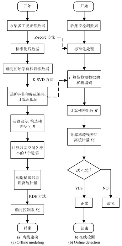
SRD方法分为离线建模和在线检测两部分.
1.2.1 离线建模
1) 收集多工况正常数据矩阵$X$, 使用$Z$-score方法对$X$进行标准化处理, 得到矩阵$X'$;
2) 确定初始字典$D$和训练数据$X_{\rm tr}$, 根据式(2)获得与$D$对应的稀疏编码$A$, 使用训练数据更新$D$和$A$, 得到更准确表达数据特征的字典$\hat{D}$和稀疏编码$\hat{A}$;
3) 由式(4)计算$X'$的近似值$\tilde{X'}$, 由式(5)得到残差, 构造残差空间$R$;
4) 将残差空间$R$的每一列看作一个样本, 根据式(6)计算各样本间$l$个近邻的距离平方和, 作为计算控制限的统计指标;
5) 使用核密度估计法求出置信水平为$\alpha$的控制限$D_{\alpha}^2$.
1.2.2 在线检测
1) 收集待检测数据, 使用建模数据的均值及方差进行标准化处理, 得到标准化后的数据矩阵为$X_{\rm new}$;
2) 保持建模时的字典不变, 根据式(2)计算矩阵$X_{\rm new}$的稀疏编码$A_{\rm new}$;
3) 由式(4)计算近似值$\hat{X}_{\rm new}$, 由式(5)得近似值与待检测数据之间的残差矩阵$R'$, 产生新的样本空间;
4) 将$R'$矩阵的每一列看作一个样本, 由式(6)计算各样本间$l$个近邻的距离平方和$D_{t}^2$;
5) 比较$D_{t}^2$与控制限$D_{\alpha}^2$的大小, 若$D_{t}^2<D_{\alpha}^2$, 则数据为正常数据, 反之, 则为故障数据.
具体流程图如图 1所示.
2. 仿真研究
2.1 数值仿真
使用的模型如下[16]:
$ \begin{align} \!\left[ \begin{array}{c} x_{1}\\ x_{2}\\ x_{3}\\ x_{4}\\ x_{5} \end{array} \right]\!= \!\left[ \begin{array}{cc} 0.5768&0.3766\\ 0.7382&0.0566\\ 0.8291&0.4009\\ 0.6519&0.2070\\ 0.3972&0.8045 \end{array} \right]\!\! \left[ \begin{array}{c} s_{1}\\ s_{2} \end{array} \right]\!+\! \left[ \begin{array}{c} e_{1}\\ e_{2}\\ e_{3}\\ e_{4}\\ e_{5} \end{array} \right]\! \end{align} $
(7) 其中, $x_{1}$、$x_{2}$、$x_{3}$、$x_{4}$、$x_{5}$为模型的5个变量, 是潜在变量, 是服从均值为0, 标准差为0.01的高斯分布的5个独立的白噪声.给出两个模态的数据代表不同工况:
$ \text{模态1:}\begin{matrix} {{s}_{1}}:Uniform(-10,-7) \\ {{s}_{2}}:\text{N}(-5,1) \\ \end{matrix} $
(8) $ \begin{align} &\text{模态2:} \begin{array}{c} s_{1}\!: Uniform(2, 5)\\ s_{2}\!: {\rm N}(7, 1) \end{array} \end{align} $
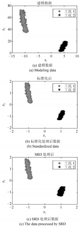
(9) 所用建模数据由两种工况分别产生400个样本组成正常训练样本集, 因此训练数据共有800个样本.随机选取训练样本中300个正常样本作为初始字典, 剩余的500个样本作为初始训练数据, 通过OMP算法得到的稀疏编码为$300\times500$维.在工况1中, $T=401$时刻起在变量$x_{5}$上加一个幅值为4的阶跃信号作为故障, 即测试数据的前400个样本为正常样本, 剩余400个样本为故障样本, 共800个样本.通过使用建模过程获得的字典计算测试数据的稀疏编码为$300\times800$维.本数值案例的稀疏距离统计量参数的选取采用交叉检验法, 选取适合的近邻个数为3.选取变量$x_{1}$和$x_{2}$两个变量方向, 分别绘制建模数据投影图、标准化处理后数据投影图和SRD处理后的数据投影图, 分别如图 2(a)、图 2(b)和图 2(c)所示.
由图 2(a)可以看出, 建模数据分为两个工况, 工况1的数据分布在30至80之间, 数据中心大约为(-10, 50), 工况2的数据分布在0至20之间, 数据中心大约为(5, 10), 数据跨度较大, 分布较散, 中心不够明确; 由图 2(b)可以看出, 标准化后, 数据依然分为两个工况, 此时工况1的中心为(-1, 1), 工况2的中心为(1, -1), 两个工况数据的中心呈中心对称; 在图 2(c)中, 数据的中心与图 2(b)一样, 与图 2(a)相比, 数据的分布形态基本一致, 且提取数据特征后的数据跨度明显减小, 数据分布相对更集中, 数据特征得到强化, 更加明显突出, 由此说明本文方法是针对具有多工况特征过程的方法.
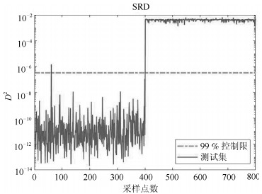
使用本文所提SRD算法的故障检测结果如图 3所示, 由图可以看出, 前400个样本基本全部位于控制限以下, 误报率为0.25%; 剩余400个样本全部位于控制限上方, 故障全部被检测出来, 漏报率为0, 说明该方法能够有效解决多工况问题.
2.2 过程仿真
TE过程是1993年由Downs和Vogel以伊斯曼化学品公司的实际工艺流程为基础, 改进后提出的一个复杂非线性过程[17], TE过程适合于研究过程控制技术、过程监控、故障检测与诊断等方向.该过程由反应器、冷凝器、压缩机、汽提塔和汽/液分离器5个主要的操作单元组成, 包括8种成分, 有6种生产模式, 如表 1所示.过程中有41个测量变量和12个控制变量, 详细的工艺流程如图 4所示.
表 1 TE过程故障Table 1 Failures of TE process故障编号 性质描述 变化类型 IDV 1 物料A/C进料比改变, 物料B含量不变 阶跃 IDV 2 物料A/C进料比不变, 物料B含量改变 阶跃 IDV 4 反应器冷却入口温度改变 阶跃 IDV 6 物料A进料损失 阶跃 IDV 7 物料C压力损失 阶跃 IDV 13 反应动力学参数改变 慢偏移 IDV 16 未知 未知 TE过程各种工况的采样频率均是3分钟/次, 每次仿真都运行48个小时.仿真从正常工况开始进行, 在仿真开始8小时后引入故障, 共有21种故障可以引入, 本文验证算法有效性采用的故障如表 1所示.本文仿真实验采用TE过程生产模式1和3, 如表 2所示, 分别代表工况1和工况2, 将两个工况的数据混合使用, 用于建模的两个工况的正常样本数为1200, 用于检测的样本数为1200, 检测的样本中包含正常数据200和故障数据1000.采用的变量为41个测量变量和12个控制变量, 共53个变量.
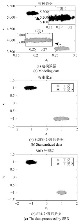
表 2 本文采用的TE过程生产模式Table 2 TE process production model used in this paper生产模式 G/H比率 产品生产率 1 50/50 7 038 kgh-1 G和7 038 kgh-1 H 3 90/10 1 000 kgh-1 G和1 111 kgh-1 H "kgh-1 G"表示"每小时生产多少千克的G产品", "kgh-1 H"表示"每小时生产多少千克的H产品". 在基于SRD的故障检测方法中, 为避免不同工况过渡过程对检测效果产生影响, 本文首先对多工况数据进行合理选取, 通过交叉检验法选取建模数据集($53\times1\, 200$).随机选取建模数据集中400个样本作为初始字典, 其维数为$53\times400$; 剩余800个样本为训练数据, 其维数为$53\times800$; 二者通过OMP计算后获得的稀疏编码为$400\times800$维.对于检测的数据集, 使用建模数据集的字典($53\times400$)计算得到的稀疏编码为$400\times1\, 200$维.为验证SRD方法能够准确提取数据特征, 任取两个变量方向分别绘制建模数据投影图、标准化处理后数据投影图和SRD处理后的数据投影图, 分别如图 5(a)、图 5(b)和图 5(c)所示.
由图 5(a)可以看出, 建模数据分为两个工况, 工况1的数据分布在3600至3750之间, 工况2的数据分布在5100至5250之间, 数据跨度较大, 分布较散, 中心不够明确, 特征不够突出; 由图 5(b)可以看出, 标准化后, 数据依然分为两个工况, 工况1的中心为(1, -1), 工况2的中心为(-1, 1);在图 5(c)中, 数据依然分为两个工况, 中心也保持不变, 工况1的数据分布在-1.3至-0.7之间, 工况2的数据分布在0.7至1.3之间, 数据跨度明显减小. 图 5(c)和图 5(a)中数据的分布形态基本一致, 而且提取数据特征后的数据分布相对更集中, 数据特征得到强化, 更加明显突出, 便于捕捉, 在此基础上构建多工况数据的故障检测统计量会更准确, 由此也说明本文方法是针对具有多工况特征过程的方法.
实验过程中, 构建稀疏距离统计量的参数$l$的选取采用交叉检验法, 通过多次试验选取合适的$l$值, 即$l=3$, 故后续实验涉及到的参数$l$均选取3.
本文验证所提SRD方法有效性的同时, 还与以SPE为统计量的KSVD-R (K-singular value decomposition residual)方法的检测结果进行了比较.以故障6和故障13为例对故障检测结果进行说明.故障6和故障13的故障检测结果如图 6、图 7所示, 从图中可以看到数据具有多工况特征, 分为两个工况, 前600个样本为工况1, 后600个样本为工况2;每一工况的前100个样本为正常样本, 后500个为故障样本.
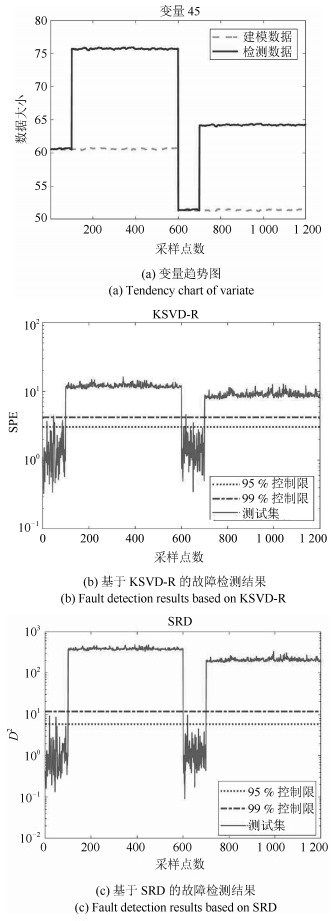
由表 1知, 故障6 (A进料损失)为阶跃故障, 经过多次试验发现变量45 (总进料量)体现阶跃最明显, 具有明显的故障特征, 视其为影响故障的主要变量, 具体趋势见图 6(a). 图 6(b)为以SPE为统计量的KSVD-R故障检测方法的故障检测结果图, 由图可知故障全部位于置信度为99%的控制限上方, 正常样本基本位于该控制限下方, 仅有少数几个样本位于其上方, 显然该方法存在误报样本. 图 6(c)为本文所提SRD方法的故障检测结果图, 由图可知故障样本全部位于置信度为99%的控制限上方, 正常样本全部位于该控制限下方, 显然SRD方法误报率极低, 趋近于0.将图 6(a)和图 6(c)进行比较, 可以看出, 数据趋势基本一致, 说明SRD算法可以在保证数据结构、工况特征不变的基础上进行故障检测.将图 6(b)和图 6(c)进行比较, 可以看出SRD方法的误报样本少于KSVD-R方法, 且SRD方法正常样本和故障样本数值差距稍大, 说明在残差空间引入的距离统计量确实能够使故障样本和正常样本区分更加明显.
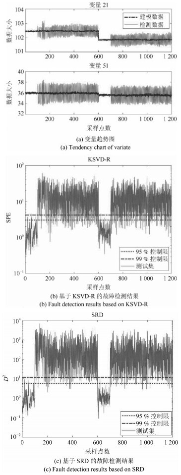
由表 1知, 故障13 (反应动态)为慢偏移故障, 经过多次试验发现变量21 (反应器冷却水出口温度)和变量51 (反应器冷却水流量)具有明显的数据特征, 视其为影响故障的主要变量, 具体趋势见图 7(a). 图 7(b)为KSVD-R方法的故障检测结果图, 由图可见大部分故障位于置信度为99%的控制限上方, 正常样本基本位于该控制限下方, 仅有少数几个样本位于其上方, 显然该方法存在误报样本和漏报样本.
图 7(c)为SRD方法的故障检测结果图, 由图可知绝大部分故障样本位于置信度为99%的控制限上方, 正常样本全部位于该控制限下方, 显然SRD方法检测率更高, 误报率更低.将图 7(a)和图 7(c)进行比较, 可以看出, 数据趋势基本一致, 再次验证SRD方法可以保持原始数据特征.将图 7(b)和图 7(c)进行比较, 可以看出SRD方法的误报样本明显少于KSVD-R方法, 图 7(b)中工况1的故障样本和工况2的正常样本界限模糊, 存在交叉现象, 而图 7(c)中正常样本和故障样本数值差距更大, 区分更加明显, 更加说明在残差空间引入的距离统计量确实能够使故障样本和正常样本区分更加明显.
由图 6(c)和图 7(c)可以看出, 各工况故障检测效果均良好, 说明SRD方法无需对待检测样本进行工况识别仍能够检测到不同工况的故障, 由此说明SRD方法使用的多工况数据混合建模方式是有效的, 适用于解决多工况问题.
选取几个对比较明显的故障, 将其误报率及检测率汇总成表, 如表 3所示.由表 3可以看出:
表 3 误报率及检测率汇总表Table 3 False alarm rate and detection rate summary table故障号 KSVD-R SRD 误报率(%) 检测率(%) 误报率(%) 检测率(%) 1 4.50 0.10 100 100 2.00 0 100 100 2 4.50 0.10 100 98.6 2.00 0 100 100 4 4.50 0.10 100 100 2.00 0 100 100 6 4.50 0.10 100 100 2.00 0 100 100 7 4.50 0.10 100 100 2.00 0 100 100 13 4.50 0.10 89.6 82.1 2.00 0 97.8 90.2 16 4.50 0.10 94.6 90.2 2.00 0 98.6 94.7 注1:表 3中误报率和漏报率下属两列数据, 靠前的一列为控制限为95%的数值, 靠后的一列为控制限为99%的数值 1) 对于误报率, 依据置信度为95%的控制限, 与KSVD-R方法相比, SRD方法的误报率降低了2.5%;依据置信度为99%的控制限, 则降低了0.1%;由此说明距离统计量对误报率的改进起一定作用;
2) 对于故障1、故障4、故障6、故障7, 无论使用哪种方法, 故障检测率均为100%;
3) 依据置信度为95%的控制限, 故障2、故障13、故障16使用SRD方法的故障检测率比KSVD-R方法分别提高了1.4%、8.1%、4.5%;依据置信度为99%的控制限, 故障13、故障16使用SRD方法的故障检测率比KSVD-R方法分别提高了8.2%和8.4%;进一步说明残差空间引入距离统计量确实可以改进故障检测性能.
3. 结束语
本文提出了一种新的基于稀疏分解残差距离的多工况过程故障检测方法.该方法将多工况数据混合建模, 提取数据特征, 依据获得的数据特征计算近似值及其与测量值的残差, 在残差空间首次引入$k$最近邻距离统计量进行故障检测. SRD方法与KSVD-R方法相比, 故障检测效果有明显提高.同时该方法可以避免进行线性化、高斯化、分工况等数据预处理, 提高了多工况过程故障检测的有效性.将SRD方法运用于多工况过程的故障定位、故障分类将是进一步研究的内容.
-
[1] Wei X J, Wu Z J, Hamid R K. Disturbance observerbased disturbance attenuation control for a class of stochastic systems. Automatica, 2016, 63: 21−25 doi: 10.1016/j.automatica.2015.10.019 [2] 魏新江, 孙式香, 张慧凤. 随机多源干扰系统的复合DOBC和容错 控制. 控制与决策, 2019, 34(3): 668−672Wei Xin-Jiang, Sun Shi-Xiang, Zhang Hui-Feng. Faulttolerant control based on disturbance observer for stochastic systems with multiple disturbances. Control and Decision, 2019, 34(3): 668−672 [3] Li Y K, Chen M, Cai L, Wu Q X. Resilient control based on disturbance observer for nonlinear singular stochastic hybrid system with partly unknown Markovian jump parameters. Journal of the Franklin Institute, 2018, 355(5): 2243−2265 doi: 10.1016/j.jfranklin.2017.12.038 [4] Wei X J, Sun S X. Elegant anti-disturbance control for discrete-time stochastic systems with nonlinearity and multiple disturbances. International Journal of Control, 2017, 91(3): 706−714 [5] Wei X J, Zhang H F, Sun S X, Hamid R K. Composite hierarchical anti-disturbance control for a class of discretetime stochastic systems. International Journal of Robust and Nonlinear Control, 2018, 28(9): 3292−3302 doi: 10.1002/rnc.4080 [6] Zong G D, Li Y, Sun H B. Composite anti-disturbance resilient control for Markovian jump nonlinear systems with general uncertain transition rate. Science China Information Sciences, 2019, 62(2): 101−118 [7] 司文杰, 董训德, 王聪. 输入饱和的一类切换系统神经网络跟踪控 制. 自动化学报, 2017, 43(8): 1383−1392Si Wen-Jie, Dong Xun-De, Wang Cong. Adaptive neural tracking control design for a class of uncertain switched nonlinear systems with input saturation. Acta Automatica Sinica, 2017, 43(8): 1383−1392 [8] 林安辉, 蒋德松, 曾建平. 具有输入饱和的欠驱动船舶编队控制. 自 动化学报, 2018, 44(8): 1496−1504Lin An-Hui, Jiang De-Song, Zeng Jian-Ping. Underactuated ship formation control with input saturation. Acta Automatica Sinica, 2018, 44(8): 1496−1504 [9] 王萌, 孙雷, 尹伟, 等. 面向交互应用的串联弹性驱动器力矩控制方 法. 自动化学报, 2017, 43(8): 1319−1328Wang Meng, Sun Lei, Yin Wei, et al. Series elastic actuator torque control approach for interaction application. Acta Automatica Sinica, 2017, 43(8): 1319−1328 [10] Sui S, Tong S, Li Y. Observer-based fuzzy adaptive prescribed performance tracking control for nonlinear stochastic systems with input saturation. Neurocomputing, 2015, 158: 100−108 doi: 10.1016/j.neucom.2015.01.063 [11] Si W, Dong X, Si W, et al. Adaptive neural control for MIMO stochastic nonlinear purefeedback systems with input saturation and full-state constraints. Neurocomputing, 2018, 275(31):298−307 [12] Dong L W, Wei X J, Zhang H F. Anti-disturbance control based on nonlinear disturbance observer for a class of stochastic systems. Transactions of the Institute of Measurement and Control, 2019, 41(6): 1665−1675 doi: 10.1177/0142331218787608 [13] Bernt K O. Stochastic Differential Equations: An Introduction with Applications, Berlin: Springer-Verlag, 2002. [14] Kozin F. A survey of stability of stochastic systems. Automatica, 1969, 5(1): 95−112 doi: 10.1016/0005-1098(69)90060-0 [15] Mao X R, Yuan C G. Stochastic Differential Equations with Markovian Switching. London: Imperial College Press, 2006, 157−158 -


 下载:
下载:

 下载:
下载:

计量
- 文章访问数: 1261
- HTML全文浏览量: 291
- PDF下载量: 286
- 被引次数: 0
