

Research on Property-based Distributed Low Carbon Parallel Machines Scheduling Algorithm
-
摘要: 针对分布式低碳并行机调度问题(Distributed low carbon parallel machine scheduling problem, DLCPMSP), 由于该问题子问题众多, 为此, 首先将问题转换为扩展的低碳不相关并行机调度问题以降低子问题的数量; 然后提出了一种基于问题性质的非劣排序遗传算法-Ⅱ(Property-based non-dominated sorting genetic algorithm-Ⅱ, PNSGA-Ⅱ)以同时最优化总延迟时间和总能耗, 该算法运用针对问题特征的两种启发式算法初始化种群, 给出了问题的四种性质及证明, 提出了两种基于问题性质的局部搜索方法.运用大量实例进行了算法策略分析和对比实验, 结果分析表明, PNSGA-Ⅱ在求解DLCPMSP方面具有较强优势.Abstract: In this study distributed low carbon parallel machine scheduling problem (DLCPMSP) is considered. Owing to many sub-problems, DLCPMSP is transformed into an extended low carbon unrelated parallel machine scheduling problem to diminish the number of sub-problems. A property-based non-dominated sorting genetic algorithm-Ⅱ (PNSGA-Ⅱ) is proposed to minimize total tardiness and total energy consumption. In PNSGA-Ⅱ, two heuristics based on problem features of the problem are used to initialize population, four properties and related proofs are given and two property-based local searches are applied. Many experiments are conducted to show the effect of strategies and compare PNSGA-Ⅱ with other algorithms from literature. Computational results validate that PNSGA-Ⅱ has strong advantages for solving DLCPMSP.
-
Key words:
- Distributed scheduling /
- low carbon scheduling /
- heuristic /
- problem property
1) 本文责任编委 伍洲 -

图 3 6种算法关于四个实例的非劣解分布
Fig. 3 Distribution of non-dominated solutions of six algorithms on four instances
表 1 参数各水平取值
Table 1 Factor levels of parameters
参数 水平 1 2 3 4 $p_c$ 0.80 0.85 0.90 95 $p_m$ 0.00 0.05 0.10 0.15 $N$ 60 90 120 150  下载: 导出CSV
表 2 参数正交表及$DI_R$值
Table 2 Orthogonal array and $DI_R$ value
No. Factor $DI_R$ $p_c$ $p_m$ $N$ 1 1 1 1 20.94 2 1 2 2 13.42 3 1 3 3 6.012 4 1 4 4 6.519 5 2 1 2 19.85 6 2 2 1 13.82 7 2 3 4 6.721 8 2 4 3 6.000 9 3 1 3 11.89 10 3 2 4 8.126 11 3 3 1 10.68 12 3 4 2 6.536 13 4 1 4 11.13 14 4 2 3 8.531 15 4 3 2 8.199 16 4 4 1 14.84
下载: 导出CSV
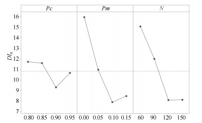
表 3 各参数平均$DI_R$
Table 3 Average $DI_R$ of factors
水平 $p_c$ $p_m$ $N$ 1 11.72 15.95 15.07 2 11.60 10.97 12.00 3 9.308 7.903 8.108 4 10.68 8.474 8.124 Delta 2.415 8.050 6.962 排秩 3 1 2
下载: 导出CSV
表 4 种算法关于指标$DI_R$的对比
Table 4 Comparisons of six algorithms on metric $DI_R$
实例 PNSGA-Ⅱ A1 A2 NSGA-Ⅱ SPEA2 TIPG $2\times 10$ 1.009 5.989 3.753 13.50 1.147 29.95 $2\times 20$ 0.281 6.376 3.388 7.796 4.388 53.21 $2\times 30$ 0.297 6.272 3.361 9.465 5.240 47.96 $2\times 40$ 0.730 5.559 1.714 6.074 4.894 68.06 $3\times 40$ 0.074 6.583 0.676 7.432 6.269 63.24 $4\times 40$ 0.138 9.122 3.640 11.81 9.682 75.89 $2\times 50$ 0.933 9.606 2.045 8.024 12.73 72.65 $3\times 50$ 0.575 4.534 2.159 9.229 9.567 82.67 $4\times 50$ 0.045 7.053 2.243 8.349 7.639 83.56 $2\times 60$ 1.352 9.857 0.897 9.036 9.905 73.18 $3\times 60$ 0.866 5.166 1.608 6.861 7.685 73.38 $4\times 60$ 0.257 8.610 0.944 9.485 10.09 77.30 $2\times 80$ 1.851 8.616 0.871 9.539 14.04 83.09 $3\times 80$ 0.932 8.299 0.979 10.08 11.30 84.17 $4\times 80$ 1.017 14.53 0.594 16.18 18.06 98.23 $5\times 80$ 0.591 12.02 0.512 11.77 14.91 91.74 $2\times 100$ 1.611 5.917 1.996 6.714 10.73 76.21 $3\times 100$ 0.234 6.328 1.295 7.729 11.84 83.59 $4\times 100$ 0.083 7.440 1.079 11.53 15.13 88.09 $5\times 100$ 1.299 13.47 0.565 13.46 17.34 88.42 $2\times 200$ 1.664 21.42 2.198 28.48 36.18 $-$ $3\times 200$ 2.808 39.37 1.559 45.69 56.06 $-$ $4\times 200$ 0.640 33.89 1.886 38.96 48.04 $-$ $5\times 200$ 0.291 34.63 3.118 36.65 54.36 $-$ 均值 0.816 12.11 1.795 14.33 16.55 74.73
下载: 导出CSV
表 5 6种算法关于指标$\rho $的结果对比
Table 5 Comparisons of six algorithms on metric $\rho $
实例 PNSGA-Ⅱ A1 A2 NSGA-Ⅱ SPEA2 TIPG $2\times 10$ 0.444 0.111 0.000 0.000 0.556 0.000 $2\times 20$ 0.583 0.021 0.333 0.021 0.083 0.000 $2\times 30$ 0.975 0.025 0.000 0.000 0.012 0.000 $2\times 40$ 0.847 0.020 0.053 0.067 0.020 0.000 $3\times 40$ 0.910 0.010 0.080 0.000 0.010 0.000 $4\times 40$ 0.710 0.011 0.290 0.000 0.000 0.000 $2\times 50$ 0.718 0.137 0.076 0.046 0.031 0.000 $3\times 50$ 0.872 0.032 0.106 0.000 0.000 0.000 $4\times 50$ 0.896 0.015 0.104 0.000 0.000 0.000 $2\times 60$ 0.840 0.024 0.080 0.032 0.032 0.000 $3\times 60$ 0.822 0.059 0.129 0.000 0.000 0.000 $4\times 60$ 0.793 0.009 0.198 0.000 0.009 0.000 $2\times 80$ 0.551 0.059 0.324 0.074 0.000 0.000 $3\times 80$ 0.632 0.008 0.361 0.000 0.008 0.000 $4\times 80$ 0.646 0.015 0.354 0.000 0.000 0.000 $5\times 80$ 0.648 0.014 0.352 0.000 0.000 0.000 $2\times 100$ 0.759 0.036 0.015 0.197 0.000 0.000 $3\times 100$ 0.912 0.054 0.039 0.000 0.000 0.000 $4\times 100$ 0.897 0.015 0.088 0.004 0.000 0.000 $5\times 100$ 0.480 0.010 0.520 0.000 0.000 0.000 $2\times 200$ 0.853 0.041 0.086 0.024 0.000 $-$ $3\times 200$ 0.765 0.008 0.212 0.019 0.000 $-$ $4\times 200$ 0.852 0.004 0.148 0.000 0.000 $-$ $5\times 200$ 0.926 0.005 0.074 0.000 0.000 $-$ 均值 0.764 0.031 0.168 0.020 0.032 0.000
下载: 导出CSV
表 6 6种算法关于指标$SP$的结果对比
Table 6 Comparisons of six algorithms on metric $SP$
实例 PNSGA-Ⅱ A1 A2 NSGA-Ⅱ SPEA2 TIPG $2\times 10$ 1.127 3.207 4.554 14.68 2.784 7.470 $2\times 20$ 5.067 7.465 8.554 11.71 6.242 10.89 $2\times 30$ 5.036 13.77 10.95 8.816 14.22 18.55 $2\times 40$ 5.991 11.06 8.533 8.843 8.173 32.89 $3\times 40$ 6.477 8.199 10.12 9.624 6.823 13.56 $4\times 40$ 11.62 6.939 7.778 28.52 7.423 13.82 $2\times 50$ 10.94 6.345 14.26 13.60 16.32 21.35 $3\times 50$ 7.455 6.917 13.66 11.19 8.641 9.448 $4\times 50$ 8.089 9.014 27.52 10.73 8.114 24.12 $2\times 60$ 6.587 15.73 9.264 8.064 10.17 14.75 $3\times 60$ 9.447 12.27 17.74 13.22 8.957 13.86 $4\times 60$ 20.60 17.81 10.13 14.20 7.310 9.080 $2\times 80$ 13.98 13.50 8.977 10.19 6.923 36.90 $3\times 80$ 17.02 16.83 8.464 14.67 10.77 13.87 $4\times 80$ 4.881 17.26 10.34 17.97 7.760 12.32 $5\times 80$ 6.401 12.19 11.54 17.18 11.84 19.29 $2\times 100$ 11.78 12.92 17.65 37.68 38.74 101.1 $3\times 100$ 22.38 19.90 15.50 14.32 14.00 15.60 $4\times 100$ 10.31 16.27 12.09 10.93 20.60 26.28 $5\times 100$ 4.997 10.20 46.75 12.72 7.564 20.12 $2\times 200$ 20.37 22.10 53.72 16.08 41.22 $-$ $3\times 200$ 8.388 34.40 18.14 19.98 25.37 $-$ $4\times 200$ 23.68 36.78 18.37 23.00 32.56 $-$ $5\times 200$ 24.12 28.59 20.19 33.74 11.76 $-$ 均值 11.11 14.99 16.03 15.90 13.93 21.77
下载: 导出CSV
表 7 配对样本$t$-test
Table 7 Paired-sample $t$-test
$t$-test experiment $p-$值$\left(DI_R\right)$ $p-$值$\left(\rho \right)$ $p-$值$\left(SP\right)$ $t$-test (PNSGA-Ⅱ, A1) 0.000 0.000 0.007 $t$-test (PNSGA-Ⅱ, A2) 0.001 0.000 0.048 $t$-test (PNSGA-Ⅱ, NSGA-Ⅱ) 0.000 0.000 0.005 $t$-test (PNSGA-Ⅱ, SPEA2) 0.000 0.000 0.148 $t$-test (PNSGA-Ⅱ, TIPG) 0.000 0.000 0.014
下载: 导出CSV
-
[1] Cheng T C E, Sin C C S. A state-of-the-art review of parallel-machine scheduling research. European Journal of Operational Research, 1990, 47(3): 271-292 [2] 王凌, 王晶晶, 吴楚格.绿色车间调度优化研究进展.控制与决策, 2018, 33(3): 385-391 http://www.wanfangdata.com.cn/details/detail.do?_type=perio&id=kzyjc201803001Wang Ling, Wang Jing-Jing, Wu Chu-Ge. Advances in green shop scheduling and optimization. Control and Decision, 2018, 33(3): 385-391 http://www.wanfangdata.com.cn/details/detail.do?_type=perio&id=kzyjc201803001 [3] Li K, Zhang X, Leung J Y T, Yang S L. Parallel machine scheduling problems in green manufacturing industry. Journal of Manufacturing Systems, 2016, 38: 98-106 http://www.wanfangdata.com.cn/details/detail.do?_type=perio&id=1b1d4c8bcc6bb0b76950e2d31d6daee2 [4] Wang S J, Wang X D, Yu J B, Ma S, Liu M. Bi-objective identical parallel machine scheduling to minimize total energy consumption and makespan. Journal of Cleaner Production, 2018, 193: 424-440 http://www.wanfangdata.com.cn/details/detail.do?_type=perio&id=eb7bc4ea618ba7c377ab7388475f30e3 [5] Wu X Q, Che A D. A memetic differential evolution algorithm for energy-efficient parallel machine scheduling. Omega, 2019, 82: 155-165 http://www.wanfangdata.com.cn/details/detail.do?_type=perio&id=a20a2c052677b71255873c01b1ffd8d8 [6] Zheng X L, Wang L. A collaborative multiobjective fruit fly optimization algorithm for the resource constrained unrelated parallel machine green scheduling problem. IEEE Transactions on Systems, Man, and Cybernetics: Systems, 2018, 48(5): 790-800 http://ieeexplore.ieee.org/document/7605452 [7] Liang P, Yang H D, Liu G S, Guo J H. An ant optimization model for unrelated parallel machine scheduling with energy consumption and total tardiness. Mathematical Problems in Engineering, 2015, 2015: Article No. 907034 [8] Li Z T, Yang H D, Zhang S Q, Liu S Q. Unrelated parallel machine scheduling problem with energy and tardiness cost. The International Journal of Advanced Manufacturing Technology, 2016, 84(1): 213-226 http://www.wanfangdata.com.cn/details/detail.do?_type=perio&id=c055c9d705e004ac44af028f54031ce3 [9] Che A D, Zhang S B H, Wu X Q. Energy-conscious unrelated parallel machine scheduling under time-of-use electricity tariffs. Journal of Cleaner Production, 2017, 156: 688-697 http://www.wanfangdata.com.cn/details/detail.do?_type=perio&id=d073310b588cea264bb80c94121662c0 [10] 雷德明, 潘子肖, 张清勇.多目标低碳并行机调度研究.华中科技大学学报(自然科学版), 2018, 46(8): 104-109 http://www.wanfangdata.com.cn/details/detail.do?_type=perio&id=hzlgdxxb201808020Lei De-Ming, Pan Zi-Xiao, Zhang Qing-Yong. Researches on multi-objective low carbon parallel machines scheduling. Journal of Huazhong University of Science and Technology (Natural Science Edition), 2018, 46(8): 104-109 http://www.wanfangdata.com.cn/details/detail.do?_type=perio&id=hzlgdxxb201808020 [11] Guo Z X, Ngai E W T, Yang C, Liang X D. An RFID-based intelligent decision support system architecture for production monitoring and scheduling in a distributed manufacturing environment. International Journal of Production Economics, 2015, 159: 16-28 http://www.wanfangdata.com.cn/details/detail.do?_type=perio&id=df53b2567919bf7afc9a0e70cc824e01 [12] Lee C K, Shen Y A, Yang T, Tang A L. An effective two-phase approach in solving a practical multi-site order scheduling problem. Journal of the Chinese Institute of Industrial Engineers, 2011, 28(7): 543-552 http://www.wanfangdata.com.cn/details/detail.do?_type=perio&id=10.1080/10170669.2011.637579 [13] Gnoni M G, Iavagnilio R, Mossa G, Mummolo G, Di Leva A. Production planning of a multi-site manufacturing system by hybrid modelling: A case study from the automotive industry. International Journal of Production Economics, 2003, 85(2): 251-262 http://www.sciencedirect.com/science/article/pii/S0925527303001130 [14] Timpe C H, Kallrath J. Optimal planning in large multi-site production networks. European Journal of Operational Research, 2000, 126(2): 422-435 http://www.wanfangdata.com.cn/details/detail.do?_type=perio&id=5bcdacd526ebaf6e7dbfd1e00c3c92c5 [15] Behnamian J, Fatemi Ghomi S M T. A survey of multi-factory scheduling. Journal of Intelligent Manufacturing, 2016, 27(1): 231-249 http://www.wanfangdata.com.cn/details/detail.do?_type=perio&id=e98c9e9ebb9852aba68e057b1b492b85 [16] 王凌, 邓瑾, 王圣尧.分布式车间调度优化算法研究综述.控制与决策, 2016, 31(1): 1-11 http://www.wanfangdata.com.cn/details/detail.do?_type=perio&id=kzyjc201601001Wang Ling, Deng Jin, Wand Sheng-Yao. Survey on optimization algorithms for distributed shop scheduling. Control and Decision, 2016, 31(1): 1-11 http://www.wanfangdata.com.cn/details/detail.do?_type=perio&id=kzyjc201601001 [17] Chen Z L, Pundoor G. Order assignment and scheduling in a supply chain. Operations Research, 2006, 54(3): 555-572 http://dl.acm.org/citation.cfm?id=1246577 [18] Terrazas-Moreno S, Grossmann I E. A multiscale decomposition method for the optimal planning and scheduling of multi-site continuous multiproduct plants. Chemical Engineering Science, 2011, 66(19): 4307-4318 http://www.wanfangdata.com.cn/details/detail.do?_type=perio&id=52e76902534a683e4ca757e03e50bc3a [19] Behnamian J, Fatemi Ghomi S M T. The heterogeneous multi-factory production network scheduling with adaptive communication policy and parallel machine. Information Sciences, 2013, 219: 181-196 http://www.wanfangdata.com.cn/details/detail.do?_type=perio&id=283e7956c2449a0f11d78199dee4914f [20] Behnamian J. Decomposition based hybrid VNS-TS algorithm for distributed parallel factories scheduling with virtual corporation. Computers & Operations Research, 2014, 52: 181-191 http://www.wanfangdata.com.cn/details/detail.do?_type=perio&id=f25e3e0042841ec15565128b12cd35e5 [21] Behnamian J, Fatemi Ghomi S M T. Minimizing cost-related objective in synchronous scheduling of parallel factories in the virtual production network. Applied Soft Computing, 2015, 29: 221-232 http://www.wanfangdata.com.cn/details/detail.do?_type=perio&id=f9cebf0fa53df4bc4f147bc6748eff9e [22] Deb K, Agrawal S, Pratap A, Meyarivan T. A fast elitist non-dominated sorting genetic algorithm for multi-objective optimization: NSGA-Ⅱ. In: Proceedings of the 6th International Conference on Parallel Problem Solving From Nature. Paris, France: Springer, 2000. 849-858 [23] Wang Y, Zhang J, Assogba K, Liu Y, Xu M Z, Wang Y H. Collaboration and transportation resource sharing in multiple centers vehicle routing optimization with delivery and pickup. Knowledge-Based Systems, 2018, 160: 296-310 http://www.wanfangdata.com.cn/details/detail.do?_type=perio&id=3715dbf73dfa30fc4a3c51ec5813aaec [24] Vahdani B, Veysmoradi D, Shekari N, Mousavi S M. Multi-objective, multi-period location-routing model to distribute relief after earthquake by considering emergency roadway repair. Neural Computing and Applications, 2018, 30(3): 835-854 http://www.wanfangdata.com.cn/details/detail.do?_type=perio&id=7e2dfdf089a6235c7258ca4f74ab5d18 [25] Nedjati A, Izbirak G, Arkat J. Bi-objective covering tour location routing problem with replenishment at intermediate depots: Formulation and meta-heuristics. Computers & Industrial Engineering, 2017, 110: 191-206 http://www.sciencedirect.com/science/article/pii/S0360835217302565 [26] Camara M V O, Ribeiro G M, Tosta M D C R. A pareto optimal study for the multi-objective oil platform location problem with NSGA-Ⅱ. Journal of Petroleum Science and Engineering, 2018, 169: 258-268 http://www.sciencedirect.com/science/article/pii/S0920410518304297 [27] Sun Y, Lin F H, Xu H T. Multi-objective optimization of resource scheduling in fog computing using an improved NSGA-Ⅱ. Wireless Personal Communications, 2018, 102(2): 1369-1385 doi: 10.1007/s11277-017-5200-5 [28] Afzalirad M, Rezaeian J. A realistic variant of bi-objective unrelated parallel machine scheduling problem: NSGA-Ⅱ and MOACO approaches. Applied Soft Computing, 2017, 50: 109-123 [29] Sofia A S, GaneshKumar P. Multi-objective task scheduling to minimize energy consumption and makespan of cloud computing using NSGA-Ⅱ. Journal of Network and Systems Management, 2018, 26(2): 463-485 doi: 10.1007/s10922-017-9425-0 [30] Wang H F, Fu Y P, Huang M, Huang G O, Wang J W. A NSGA-Ⅱ based memetic algorithm for multiobjective parallel flowshop scheduling problem. Computers & Industrial Engineering, 2017, 113: 185-194 [31] Yang Y, Cao L C, Wang C C, Zhou Q, Jiang P. Multi-objective process parameters optimization of hot-wire laser welding using ensemble of metamodels and NSGA-Ⅱ. Robotics and Computer-Integrated Manufacturing, 2018, 53: 141-152 http://www.zhangqiaokeyan.com/academic-journal-foreign_other_thesis/0204112722649.html [32] Wang S, Ali S, Yue T, Liaaen M. Integrating weight assignment strategies with NSGA-Ⅱ for supporting user preference multiobjective optimization. IEEE Transactions on Evolutionary Computation, 2018, 22(3): 378-393 http://ieeexplore.ieee.org/document/8123878 [33] 陈志旺, 白锌, 杨七, 黄兴旺, 李国强.区间多目标优化中决策空间约束、支配及同序解筛选策略.自动化学报, 2015, 41(12): 2115-2124 doi: 10.16383/j.aas.2015.c150218Chen Zhi-Wang, Bai Xin, Yang Qi, Huang Xing-Wang, Li Guo-Qiang. Strategy of constraint, dominance and screening solutions with same sequence in decision space for interval multi-objective optimization. Acta Automatica Sinica, 2015, 41(12): 2115-2124 doi: 10.16383/j.aas.2015.c150218 [34] 乔俊飞, 韩改堂, 周红标.基于知识的污水生化处理过程智能优化方法.自动化学报, 2017, 43(6): 1038-1046 doi: 10.16383/j.aas.2017.c170088Qiao Jun-Fei, Han Gai-Tang, Zhou Hong-Biao. Knowledge-based intelligent optimal control for wastewater biochemical treatment process. Acta Automatica Sinica, 2017, 43(6): 1038-1046 doi: 10.16383/j.aas.2017.c170088 [35] Wang J J, Wang L. A knowledge-based cooperative algorithm for energy-efficient scheduling of distributed flow-shop. IEEE Transactions on Systems, Man, and Cybernetics: Systems, 2020, 50(5): 1805-1819 [36] Wang L, Zheng X L. A knowledge-guided multi-objective fruit fly optimization algorithm for the multi-skill resource constrained project scheduling problem. Swarm and Evolutionary Computation, 2018, 38: 54-63 http://www.wanfangdata.com.cn/details/detail.do?_type=perio&id=4d6268ff7cda6f1d66bebc9b2ce848ee [37] Karimi H, Rahmati S H A, Zandieh M. An efficient knowledge-based algorithm for the flexible job shop scheduling problem. Knowledge-Based Systems, 2012, 36: 236-244 http://www.wanfangdata.com.cn/details/detail.do?_type=perio&id=c36d7e479c958023975a2ee40f793983 [38] Gao J Q, He G X, Wang Y S. A new parallel genetic algorithm for solving multiobjective scheduling problems subjected to special process constraint. The International Journal of Advanced Manufacturing Technology, 2009, 43(1-2): 151-160 http://www.wanfangdata.com.cn/details/detail.do?_type=perio&id=5bd04960a3def4f838355a47fc3ba1d8 [39] Knowles J, Corne D. On metrics for comparing nondominated sets. In: Proceedings of the 2002 Congress on Evolutionary Computation. Honolulu, USA: IEEE, 2002. 711-716 [40] Lei D M. Pareto archive particle swarm optimization for multi-objective fuzzy job shop scheduling problems. The International Journal of Advanced Manufacturing Technology, 2008, 37(1-2): 157-165 http://www.wanfangdata.com.cn/details/detail.do?_type=perio&id=2fc7730d349fa83780e3e8c9e79c6c13 [41] Wang L, Wang S Y, Zheng X L. A hybrid estimation of distribution algorithm for unrelated parallel machine scheduling with sequence-dependent setup times. IEEE/CAA Journal of Automatica Sinica, 2016, 3(3): 235-246 [42] Zitzler E, Laumanns M, Thiele L. SPEA2: Improving the strength Pareto evolutionary algorithm. In: Proceedings of Evolutionary Methods for Design, Optimization and Control with Applications to Industrial Problems. Lausanne, Switzerland, 2001. 95-100 [43] Lin S W, Ying K C, Wu W J, Chiang Y I. Multi-objective unrelated parallel machine scheduling: A Tabu-enhanced iterated Pareto greedy algorithm. International Journal of Production Research, 2016, 54(4): 1110-1121 -

 下载:
下载:

计量
- 文章访问数: 1935
- HTML全文浏览量: 329
- PDF下载量: 153
- 被引次数: 0
