

Research Progress on Batch Normalization of Deep Learning and Its Related Algorithms
-
摘要: 深度学习已经广泛应用到各个领域, 如计算机视觉和自然语言处理等, 并都取得了明显优于早期机器学习算法的效果. 在信息技术飞速发展的今天, 训练数据逐渐趋于大数据集, 深度神经网络不断趋于大型化, 导致训练越来越困难, 速度和精度都有待提升. 2013年, Ioffe等指出训练深度神经网络过程中存在一个严重问题: 中间协变量迁移(Internal covariate shift), 使网络训练过程对参数初值敏感、收敛速度变慢, 并提出了批归一化(Batch normalization, BN)方法, 以减少中间协变量迁移问题, 加快神经网络训练过程收敛速度. 目前很多网络都将BN作为一种加速网络训练的重要手段, 鉴于BN的应用价值, 本文系统综述了BN及其相关算法的研究进展. 首先对BN的原理进行了详细分析. BN虽然简单实用, 但也存在一些问题, 如依赖于小批量数据集的大小、训练和推理过程对数据处理方式不同等, 于是很多学者相继提出了BN的各种相关结构与算法, 本文对这些结构和算法的原理、优势和可以解决的主要问题进行了分析与归纳. 然后对BN在各个神经网络领域的应用方法进行了概括总结, 并且对其他常用于提升神经网络训练性能的手段进行了归纳. 最后进行了总结, 并对BN的未来研究方向进行了展望.Abstract: Deep learning has been widely applied to various fields, such as computer vision and natural language processing, and has achieved much better results than earlier machine learning. Today, with the rapid development of information technology, deep neural networks are trained with larger data sets, and the network depth is deepening, making training complicated and speed or accuracy need to be improved. In 2013, Ioffe et al. pointed out that there is a serious problem in the training process of deep neural network, i.e., internal covariate shift. It slows down the training for requiring careful parameter initialization and smaller learning rate. Ioffe et al. put forward batch normalization (BN) to reduce the effect of internal covariate shift, to accelerate the convergence speed of training neural networks. At present, many networks use BN as an important approach to accelerate training. In view of the application value of BN, this paper systematically reviews the research progress of BN and its related algorithms. Firstly, the theory of BN is analyzed. Although BN is simple and helpful, there are also some problems, such as relying on the size of mini-batch, training and inference process are in different ways. Therefore, many scholars have proposed a variety of algorithms based on BN, the advantages and main function of those algorithms are analyzed and summarized. Then, the applications of BN in various neural network fields are summarized. And we sum up other methods to improve the training performance of neural network. At last, we give a summation to whole paper, and point out the future development tendency and research direction of BN.
-
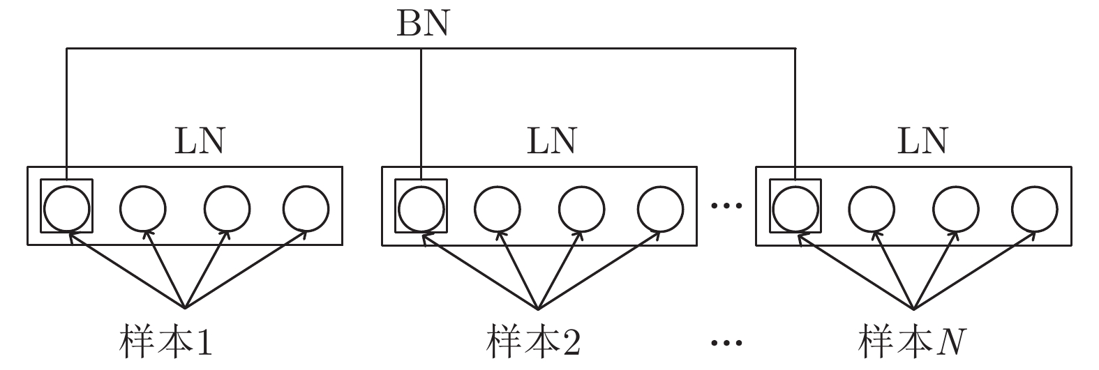
图 7 批归一化和权重归一化对比图
Fig. 7 Comparison graph of batch normalization and layer normalization
表 1 各种BN-Inception模型分类效果对比
Table 1 Comparison of classification effects of various BN-Inception models
模型 正确率达到 72.2 % 所需迭代次数 最高正确率 (%) Inception $ 31.0 \times 10^6 $ 72.2 BN-Inception $ 13.3 \times 10^6$ 72.7 BN-x5 $2.1 \times 10^6$ 73.0 BN-x30 $2.7 \times 10^6$ 74.8 BN-x5-sigmoid – 69.8  下载: 导出CSV
表 2 NIN + NP与相关模型分类效果对比 (%)
Table 2 Comparison classification effects of NIN + NP and related models (%)
模型 CIFAR-10 CIFAR-100 SVHN NIN 10.47 35.68 2.35 NIN + NP 9.11 32.19 1.88 NIN + BN 9.41 35.32 2.25 Maxout 11.68 38.57 2.47
下载: 导出CSV
表 3 使用不同
$ \alpha ^{(j)} $ 值的模型分类效果对比Table 3 Comparison of classification effects using different
$ \alpha ^{(j)}$ in model$ \alpha ^{(j)} $ MNIST NI CIFAR-10 训练周期 误差 (%) 训练周期 误差 (%) 训练周期 误差 (%) 1 52 2.70 58 7.69 45 17.31 0.75 69 1.91 67 7.37 49 17.03 0.5 69 1.84 80 7.46 44 17.11 0.25 46 1.91 38 7.32 43 17.00 0.1 48 1.90 66 7.36 48 17.10 0.01 51 1.94 74 7.47 43 16.82 0.001 48 1.95 98 7.43 46 16.28 $ 1/j $ 59 2.10 78 7.45 37 17.26 $ 1/j^2 $ 53 2.00 74 7.59 44 17.23 0 199 24.27 53 26.09 2 79.34
下载: 导出CSV
表 4 DQN + WN与DQN模型实验效果对比
Table 4 Comparison of experimental results of DQN + WN and DQN
游戏 DQN DQN + WN Breakout 410 403 Enduro 1 250 1448 Seaquest 7 188 7 357 Space invaders 1 779 2 179
下载: 导出CSV
表 5 FNN + SNN与相关模型实验效果对比(1)
Table 5 Comparing experimental results of FNN + SNN and related models (1)
模型 平均秩差 FNN + SNN −6.7 SVM −6.4 Random forest −5.9 FNN + LN −5.3
下载: 导出CSV
表 6 FNN + SNN与相关模型实验效果对比(2) (%)
Table 6 Comparing experimental results of FNN + SNN and related models (2) (%)
方法 网络层数 2 4 6 8 16 32 FNN + SNN 83.7 84.2 83.9 84.5 83.5 82.5 FNN + BN 80.0 77.2 77.0 75.0 73.7 76.0 FNN + WN 83.7 82.2 82.5 81.9 78.1 56.6 FNN + LN 84.3 84.0 82.5 80.9 78.7 78.8 FNN + ResNet 82.2 80.5 81.2 81.8 81.2 80.4
下载: 导出CSV
表 7 CNN + BN与CNN模型分类效果对比
Table 7 Comparing experimental results of CNN + BN and CNN
数据集 激活函数 模型 学习率 错误率 (%) wm50 ReLU CNN + BN 0.08 33.4 wm50 ReLU CNN 0.008 35.32 wm50 Sigmoid CNN + BN 0.08 35.52 wm50 Sigmoid CNN 0.008 42.80 wm100 ReLU CNN + BN 0.08 32.90 wm100 ReLU CNN 0.008 33.10 wm100 Sigmoid CNN + BN 0.08 33.77 wm100 Sigmoid CNN 0.008 38.50
下载: 导出CSV
表 8 LSRM + BN模型与相关模型实验效果对比
Table 8 Comparing experimental results of LSRM + BN and related models
模型 PPL 小型LSTM 78.5 小型LSTM + BN 62.5 中型LSTM 49.1 中型LSTM + BN 41.0 大型LSTM 49.3 大型LSTM + BN 35.0
下载: 导出CSV
表 9 MIM模型与相关模型实验效果对比(%)
Table 9 Comparing experimental results of MIM and related models (%)
模型 CIFAR-10 MNIST maxout 11.68 0.47 NIN 10.41 0.45 RCNN-160[67] 8.69 0.35 MIM 8.52 0.31
下载: 导出CSV
表 10 AdaBN与相关模型实验效果对比(%)
Table 10 Comparing experimental results of AdaBN and related models (%)
下载: 导出CSV
表 11 批归一化及其相关算法功能对比
Table 11 An exampletable in one column
归一化方法 收敛速度
(训练周期)计算量 优势 缺点 应用领域 未加归一化的
网络– – – – – 批归一化 (BN) 相比于未加批归一化的网络, 收敛速度加快10倍以上 适中 减少网络训练过程中的中间协变量迁移问题, 使网络训练过程对参数初始值不再敏感, 可以使用更高的学习率进行训练, 加快网络训练过程收敛速度 依赖 mini-batch 数据集的大小, 训练和推理时计算过程不同 在CNN、分片线性神经网络等FNN中效果较好, 对RNN促进效果相对较差 归一化传播 (NormProp) 比BN更稳定、收敛速度明显更快 少于BN 减少中间协变量迁移现象, 不依赖于mini-batch数据集大小, 网络中每一层的输出都服从正态分布, 训练和推理阶段计算过程相同 没有正则化效果, 也不能和其他正则化手段如Dropout
共用理论上可以应用到使用任何激活函数、目标函数的网络, 网络可以使用任何梯度传播算法进行训练, 但具体效果还需要进一步
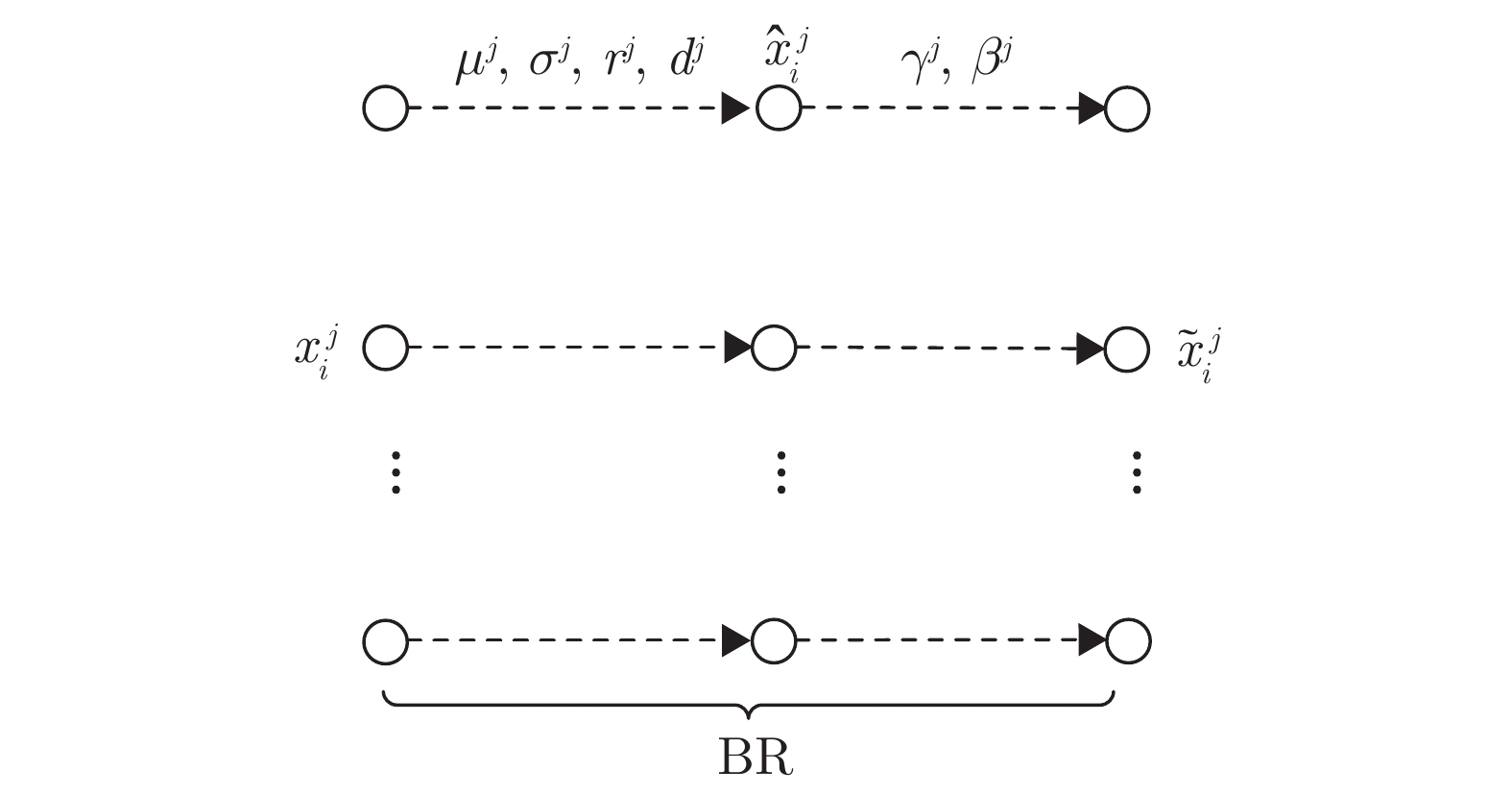
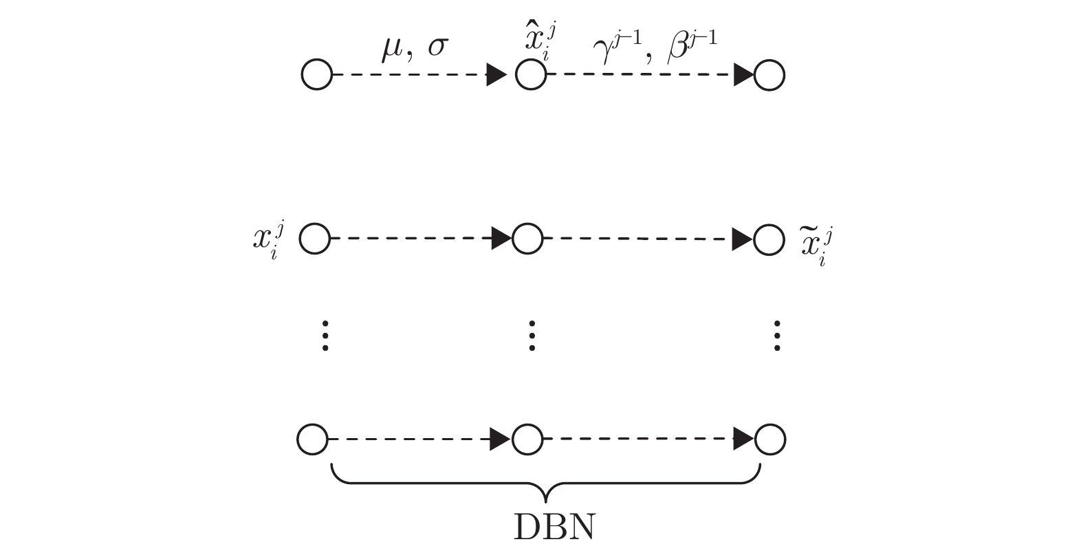
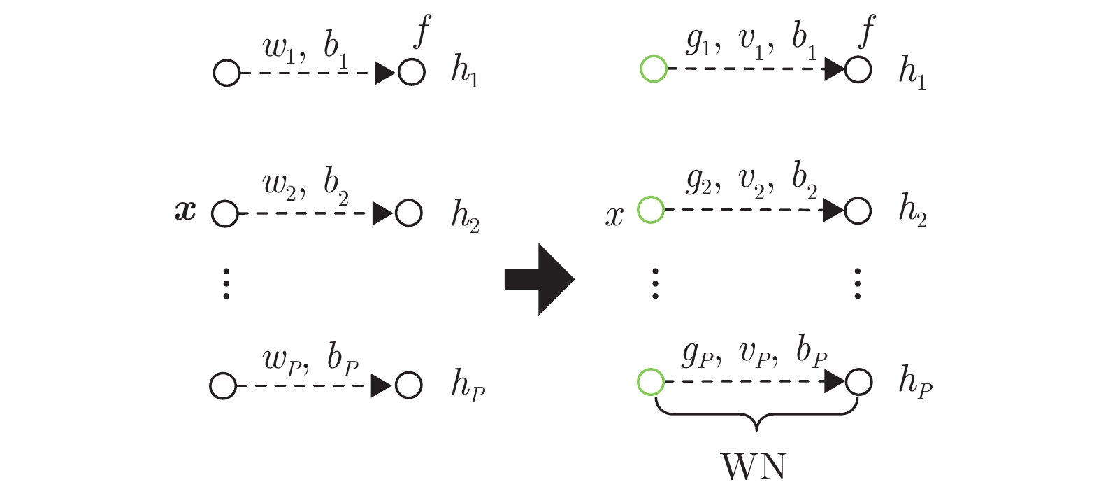
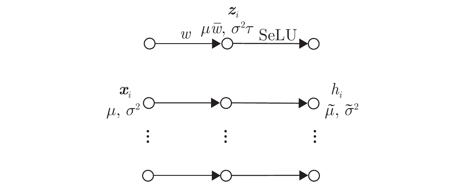
证实批量重归一化 (BR) mini-batch数据集中含有的数据量很少或包含服从非独立同分布的样本时, 比BN更稳定, 收敛更快 计算量稍多于BN 减少中间协变量迁移现象, 使网络训练对参数初值不再敏感, 可以使用更高的学习率进行训练, mini-batch中数据量很少或服从非独立同分布时, 使用BR的网络性能明显优于使用BN的网络,收敛速度更快, 训练精度更高 计算量稍多于BN 在mini-batch数据量很少或包含服从非独立同分布的样例时, 应用效果优于BN 逐步归纳批量归一化 (DBN) 比BN更稳定, 收敛速度类似BN 计算量多于BN 减少中间协变量迁移, 将神经网络的训练和推理过程关联起来, 使得网络在训练时不仅考虑当前使用的mini-batch数据集, 会同时考虑过去网络训练使用过的mini-batch数据集 对mini-batch数据集仍有一定的依赖性 理论上可以应用BN的网络, 都可以应用DBN, 但是因为没有从根本上克服BN的问题, 在应用上同样会受到一定的限制 层归一化 (LN) 比BN鲁棒性强, 收敛速度更快 计算量少于BN LN对每一层内的神经元使用单一样例进行归一化, 在训练和推理阶段计算过程相同, 应用到在线学习任务和RNN中的效果明显优于其他归一化方法, 可减少训练时间, 提升网络性能 在CNN等神经网络中的效果不如BN 层归一化对于稳定RNN中的隐层状态很有效, 可进一步推广, 但在CNN等前馈神经网络中的效果不如BN 连接边权值行向量归一化 (WN) 比BN收敛速度更快 计算量少于BN 对mini-batch数据集没有依赖性, 不需要对过去处理过的情况进行记忆, 计算复杂度低. 网络训练和推理时计算过程相同, 不会像BN一样引入过多噪声 对网络没有正则化效果 可以更好地应用到RNN和一些对噪声敏感的网络中, 如深度强化学习和深度生成式模型, 这些模型中使用BN的效果都不够好 自归一化神经网络 (SNN) – 适中 使用SeLU构造网络, 输入数据经过SNN的多层映射后, 网络中每一层输出的均值和方差可以收敛到固定点, 具有归一化特性, 网络鲁棒性强 需要使用特定的激活函数SeLU才能构成网络, 在网络中使用dropout等手段会破坏网络结构, 使网络失去自归一化特性 理论上可以构建任何前馈神经网络和递归神经网络, 但网络需要使用SeLU激活函数, 且不能破坏对数据均值和方差的逐层特征映射
下载: 导出CSV
表 12 深度神经网络加速训练方法
Table 12 Accelerated training method of deep neural network
名称 作用 代表文献 Dropout 防止网络过拟合, 是最常用的正则化方法 文献 [81—91] 正则化 防止网络过拟合 文献 [92—106] 数据增广 (Data augmentation) 通过数据变换增加训练样本数量 文献 [107—118] 改进梯度下降算法 选用合适的梯度下降算法, 更有利于神经网络训练 文献 [119—133] 激活函数选择 选择适当的激活函数, 更有利于网络训练 文献 [134—145] 学习率选择 选择适当的学习率可以加速神经网络训练 文献 [146—154] 参数初始化 好的参数初始化更易于神经网络训练 文献 [155—158] 预训练 对网络进行预训练, 适当加入先验信息, 更易于网络训练 文献 [159—162] 二值化网络 (Binarized neural networks) 节省神经网络训练过程所需存储空间和训练时间 文献 [163—167] 随机深度神经网络 缓解深度过深的神经网络训练困难的问题 文献 [168—171] 深度神经网络压缩 在不影响网络精度的情况下减少神经网络训练所需存储要求 文献 [172—178]
下载: 导出CSV
-
[1] Raina R, Madhavan A, Ng A Y. Large-scale deep unsupervised learning using graphics processors. In: Proceedings of the 26th Annual International Conference on Machine Learning. Montreal, Canada: ACM, 2009. 873−880 [2] Lecun Y A, Bottou L, Orr G B, Müller K R. Efficient BackProp. Neural Networks: Tricks of the Trade (2nd edition). New York, America: Springer, 1998. [3] Wiesler S, Richard A, Schlüter R, Ney H. Mean-normalized stochastic gradient for large-scale deep learning. In: Proceedings of the 2014 IEEE International Conference on Acoustics, Speech and Signal Processing. Florence, Italy: IEEE, 2014. 180−184 [4] Raiko T, Valpola H, Lecun Y. Deep learning made easier by linear transformations in perceptrons. In: Proceedings of the 15th International Conference on Artificial Intelligence and Statistics. La Palma, Canary Islands: JMLR, 2012. 924−932 [5] Povey D, Zhang X H, Khudanpur S. Parallel training of deep neural networks with natural gradient and parameter averaging. arXiv preprint arXiv: 1410.7455, 2014. [6] Desjardins G, Simonyan K, Pascanu R, Kavukcuoglu K. Natural neural networks. arXiv preprint arXiv: 1507.00210, 2015. [7] Ioffe S, Szegedy C. Batch normalization: Accelerating deep network training by reducing internal covariate shift. In: Proceedings of the 32nd International Conference on Machine Learning. Lille, France: JMLR.org, 2015. 448−456 [8] Silver D, Schrittwieser J, Simonyan K, Antonoglou I, Huang A, Guez A, et al. Mastering the game of Go without human knowledge. Nature, 2017, 550(7676): 354−359 doi: 10.1038/nature24270 [9] Shimodaira H. Improving predictive inference under covariate shift by weighting the log-likelihood function. Journal of Statistical Planning and Inference, 2000, 90(2): 227−244 doi: 10.1016/S0378-3758(00)00115-4 [10] Daume III H, Marcu D. Domain adaptation for statistical classifiers. Journal of Artificial Intelligence Research, 2006, 26: 101−126 doi: 10.1613/jair.1872 [11] 刘建伟, 孙正康, 罗雄麟. 域自适应学习研究进展. 自动化学报, 2014, 40(8): 1576−1600Liu Jian-Wei, Sun Zheng-Kang, Luo Xiong-Lin. Review and research development on domain adaptation learning. Acta Automatica Sinica, 2014, 40(8): 1576−1600 [12] Nair V, Hinton G E. Rectified linear units improve restricted Boltzmann machines. In: Proceedings of the 27th International Conference on Machine Learning. Madison, USA: ACM, 2010. 807−814 [13] Saxe A M, McClelland J L, Ganguli S. Exact solutions to the nonlinear dynamics of learning in deep linear neural networks. arXiv preprint arXiv: 1312.6120, 2013. [14] Devarakonda A, Naumov M, Garland M. AdaBatch: Adaptive batch sizes for training deep neural networks. arXiv preprint arXiv: 1712.02029, 2017. [15] Rifai S, Vincent P, Muller X, Glorot X, Bengio Y. Contractive auto-encoders: Explicit invariance during feature extraction. In: Proceedings of the 28th International Conference on Machine Learning. Bellevue, USA: ACM, 2011. 833−840 [16] Srivastava N, Hinton G, Krizhevsky A, Sutskever I, Salakhutdinov R. Dropout: A simple way to prevent neural networks from overfitting. Journal of Machine Learning Research, 2014, 15(56): 1929−1958 [17] Mazilu S, Iria J. L1 vs. L2 regularization in text classification when learning from labeled features. In: Proceedings of the 10th International Conference on Machine Learning and Applications and Workshops. Honolulu, Hawaii, USA: ACM, 2011. 166−171 [18] Szegedy C, Liu W, Jia Y Q, Sermanet P, Reed S, Anguelov S, et al. Going deeper with convolutions. In: Proceedings of the 2015 IEEE Conference on Computer Vision and Pattern Recognition. Boston, USA: IEEE, 2015. 1−9 [19] Sutskever I, Martens J, Dahl G, Hinton G. On the importance of initialization and momentum in deep learning. In: Proceedings of the 30th International Conference on Machine Learning. Atlanta, USA: ACM, 2013. 1139−1147 [20] Jain L P, Scheirer W J, Boult T E. Multi-class open set recognition using probability of inclusion. In: Proceedings of the 13th European Conference. Zurich, Switzerland: Springer, 2014. 393−409 [21] Arpit D, Zhou Y B, Kota B U, Govindaraju V. Normalization propagation: A parametric technique for removing internal covariate shift in deep networks. In: Proceedings of the 33rd International Conference on Machine Learning. New York, USA: ACM, 2016. 1168−1176 [22] Lin M, Chen Q, Yan S C. Network in network. arXiv preprint arXiv: 1312.4400, 2013. [23] Krizhevsky A. Learning Multiple Layers of Features from Tiny Images. Technical Report. University of Toronto, Canada, 2009. [24] Netzer Y, Wang T, Coates A, Bissacco A, Wu B, Ng A Y. Reading digits in natural images with unsupervised feature learning. NIPS Workshop on Deep Learning and Unsupervised Feature Learning, 2011, 2(5) [25] Goodfellow I J, Warde-Farley D, Mirza M, Courville A, Bengio Y. Maxout networks. arXiv preprint arXiv: 1302.4389, 2013. [26] Glorot X, Bengio Y. Understanding the difficulty of training deep feedforward neural networks. In: Proceedings of the 13th International Conference on Artificial Intelligence and Statistics. Sardinia, Italy: AISTATS, 2010. 249−256 [27] Ioffe S. Batch renormalization: Towards reducing minibatch dependence in batch-normalized models. arXiv preprint arXiv: 1702.03275, 2017. [28] Russakovsky O, Deng J, Su H, Krause J, Satheesh S, Ma S A, et al. ImageNet large scale visual recognition challenge. International Journal of Computer Vision, 2015, 115(3): 211−252 doi: 10.1007/s11263-015-0816-y [29] Goldberger J, Roweis S, Hinton G, Salakhutdinov R. Neighbourhood components analysis. In: Proceedings of the 17th International Conference on Neural Information Processing Systems. Cambridge, USA: ACM, 2004. 513−520 [30] Ma Y, Klabjan D. Convergence analysis of batch normalization for deep neural nets. arXiv preprint arXiv: 1705.08011, 2017. [31] Bottou L, Curtis F E, Nocedal J. Optimization methods for large-scale machine learning. arXiv preprint arXiv: 1606.04838, 2016. [32] Lecun Y, Bottou L, Bengio Y, Haffner P. Gradient-based learning applied to document recognition. Proceedings of the IEEE, 1998, 86(11): 2278−2324 doi: 10.1109/5.726791 [33] KDD Cup 1999 Data [Online], available: http://www.kdd.org/kdd-cup/view/kdd-cup-1999/Data, 1999. [34] Graves A, Mohamed A R, Hinton G. Speech recognition with deep recurrent neural networks. In: Proceedings of the 2013 IEEE International Conference on Acoustics, Speech, and Signal Processing. Vancouver, Canada: IEEE, 2013. 6645−6649 [35] Ba J L, Kiros J R, Hinton G E. Layer normalization. arXiv preprint arXiv: 1607.06450, 2016. [36] Vendrov I, Kiros R, Fidler S, Urtasun R. Order-embeddings of images and language. arXiv preprint arXiv: 1511.06361, 2015. [37] Graves A, Wayne G, Reynolds M, Harley T, Danihelka I, Grabska-Barwińska, et al. Hybrid computing using a neural network with dynamic external memory. Nature, 2016, 538(7626): 471−476 [38] Kiros R, Zhu Y K, Salakhutdinov R, Zemel R S, Torralba A, Urtasun R, Fidler S. Skip-thought vectors. In: Proceedings of the 28th International Conference on Neural Information Processing Systems. Quebec, Canada: ACM, 2015. 3294−3302 [39] Hermann K M, Kočiský T, Grefenstette E, Espeholt L, Kay W, Suleyman M, et al. Teaching machines to read and comprehend. In: Proceedings of the 28th International Conference on Neural Information Processing Systems. Quebec, Canada: ACM, 2015. 1693−1701 [40] Sundermeyer M, Schlüter R, Ney H. LSTM neural networks for language modeling. In: Proceedings of the 13th Annual Conference of the International Speech Communication Association. Oregon, USA: International Speech Communication Association, 2012. 194−197 [41] Gregor K, Danihelka I, Graves A, Rezende D J, Wierstra D. DRAW: A recurrent neural network for image generation. arXiv preprint arXiv: 1502.04623, 2015. [42] Salimans T, Kingma D P. Weight normalization: A simple reparameterization to accelerate training of deep neural networks. In: Proceedings of the 30th International Conference on Neural Information Processing Systems. Barcelona, Spain: ACM, 2016. 901−909 [43] Kingma D P, Welling M. Auto-encoding variational Bayes. arXiv preprint arXiv: 1312.6114, 2013. [44] Mnih V, Kavukcuoglu K, Silver D, Rusu A A, Veness J, Bellemare M G, et al. Human-level control through deep reinforcement learning. Nature, 2015, 518(7540): 529−533 doi: 10.1038/nature14236 [45] Hendrycks D, Gimpel K. Adjusting for dropout variance in batch normalization and weight initialization. arXiv preprint arXiv: 1607.02488, 2016. [46] Narayanan A, Shi E, Rubinstein B I P. Link prediction by de-anonymization: How we won the Kaggle social network challenge. In: Proceedings of the 2011 International Joint Conference on Neural Networks. San Jose, USA: IEEE, 2011. 1825−1834 [47] Cutler D R, Edwards Jr T C, Beard K H, Cutler A, Hess K T, Gibson J, Lawler J J. Random forests for classification in ecology. Ecology, 2007, 88(11): 2783−2792 doi: 10.1890/07-0539.1 [48] Joachims T. Making large-scale SVM learning practical. Advances in Kernel Methods—Support Vector Learning, 1999, 8(3): 499−526 [49] Klambauer G, Unterthiner T, Mayr A, Hochreiter S. Self-normalizing neural networks. In: Proceedings of the 31st International Conference on Neural Information Processing Systems. Long Beach, CA, USA: ACM, 2017. 972−981 [50] Fernández-Delgado M, Cernadas E, Barro S, Amorim D. Do we need hundreds of classifiers to solve real world classification problems? The Journal of Machine Learning Research, 2014, 15(1): 3133-3181 [51] Hsieh J H, Sedykh A, Huang R, Xia M H, Tice R R. A data analysis pipeline accounting for artifacts in Tox21 quantitative high-throughput screening assays. SLAS DISCOVERY: Advancing the Science of Drug Discovery, 2015, 20(7): 887−897 doi: 10.1177/1087057115581317 [52] Littwin E, Wolf L. The loss surface of residual networks: Ensembles and the role of batch normalization. arXiv preprint arXiv: 1611.02525, 2016. [53] Luo C J, Zhan J F, Wang L, Yang Q. Cosine normalization: Using cosine similarity instead of dot product in neural networks. arXiv preprint arXiv: 1702.05870, 2017. [54] Cho M, Lee J. Riemannian approach to batch normalization. In: Proceedings of the 31st International Conference on Neural Information Processing Systems. Long Beach, CA, USA: ACM, 2017. 5231−5241 [55] Wu S, Li G Q, Deng L, Liu L, Xie Y, Shi L P. L1-norm batch normalization for efficient training of deep neural networks. arXiv preprint arXiv: 1802.09769, 2018. [56] Huang L, Liu X L, Liu Y, Lang B, Tao D C. Centered weight normalization in accelerating training of deep neural networks. In: Proceedings of the 2017 IEEE International Conference on Computer Vision (ICCV). Venice, Italy: IEEE, 2017. 2822−2830 [57] Abdel-Hamid O, Mohamed A R, Jiang H, Penn G. Applying convolutional neural networks concepts to hybrid NN-HMM model for speech recognition. In: Proceedings of the 2012 IEEE International Conference on Acoustics, Speech, and Signal Processing (ICASSP). Kyoto, Japan: IEEE, 2012. 4277−4280 [58] Zhao Z Q, Bian H M, Hu D H, Cheng W J, Glotin H. Pedestrian detection based on fast R-CNN and batch normalization. In: Proceedings of the 13th International Conference on Intelligent Computing Theories and Application. Liverpool, UK: Springer, 2017. 735−746 [59] Girshick R. Fast R-CNN. In: Proceedings of the 2015 IEEE International Conference on Computer Vision (ICCV). Santiago, Chile: IEEE, 2015. [60] Darwish A, Nakhmani A. Internal covariate shift reduction in encoder-decoder convolutional neural networks. In: Proceedings of the 2017 ACM Southeast Conference. Kennesaw, USA: ACM, 2017. 179−182 [61] Laurent C, Pereyra G, Brakel P, Zhang Y, Bengio Y. Batch normalized recurrent neural networks. In: Proceedings of the 2016 IEEE International Conference on Acoustics, Speech, and signal processing (ICASSP). Shanghai, China: IEEE, 2016. 2657−2661 [62] Cooijmans T, Ballas N, Laurent C, Gülçehre Ç, Courville A. Recurrent batch normalization. arXiv preprint arXiv: 1603.09025, 2016. [63] Laurent C, Pereyra G, Brakel P, Zhang Y, Bengio Y. Batch normalized recurrent neural networks. arXiv preprint arXiv: 1510.01378, 2015. [64] Amodei D, Ananthanarayanan S, Anubhai R, Bai J L, Battenberg E, Case C, et al. Deep speech 2: End-to-end speech recognition in English and Mandarin. In: Proceedings of the 33rd International Conference on Machine Learning. New York, USA: JMLR.org, 2016. 173−182 [65] Zhang Y, Chan W, Jaitly N. Very deep convolutional networks for end-to-end speech recognition. In: Proceedings of the 2017 IEEE International Conference on Acoustics, Speech, and Signal Processing (ICASSP). New Orleans, USA: IEEE, 2017. 4845−4849 [66] Liao Z B, Carneiro G. On the importance of normalisation layers in deep learning with piecewise linear activation units. In: Proceedings of the 2016 IEEE Winter Conference on Applications of Computer Vision (WACV). Lake Placid, USA: IEEE, 2016. 1−8 [67] Liang M, Hu X L. Recurrent convolutional neural network for object recognition. In: Proceedings of the 2015 IEEE Conference on Computer Vision and Pattern Recognition (CVPR). Boston, USA: IEEE, 2015. 3367−3375 [68] Long M C, Zhu H, Wang J M, Jordan M I. Unsupervised domain adaptation with residual transfer networks. arXiv preprint arXiv: 1602. 04433, 2017. [69] Tzeng E, Hoffman J, Darrell T, Saenko K. Simultaneous deep transfer across domains and tasks. arXiv preprint arXiv: 1510. 02192, 2015. [70] Ganin Y, Lempitsky V. Unsupervised domain adaptation by backpropagation. In: Proceedings of the 32nd International Conference on Machine Learning. Lille, France: JMLR.org, 2015. 1180−1189 [71] Li Y H, Wang N Y, Shi J P, Liu J Y, Hou X D. Revisiting batch normalization for practical domain adaptation. arXiv preprint arXiv: 1603.04779, 2016. [72] Saenko K, Kulis B, Fritz M, Darrell T. Adapting visual category models to new domains. In: Proceedings of the 11th European Conference on Computer Vision. Heraklion, Greece: Springer, 2010. 213−226 [73] Gretton A, Borgwardt K M, Rasch M J, Schölkopf B, Smola A. A kernel two-sample test. The Journal of Machine Learning Research, 2012, 13: 723−773 [74] Tzeng E, Hoffman J, Zhang N, Saenko K, Darrell T. Deep domain confusion: Maximizing for domain invariance. arXiv preprint arXiv: 1412.3474, 2014. [75] Long M S, Cao Y, Wang J M, Jordan M I. Learning transferable features with deep adaptation networks. In: Proceedings of the 32nd International Conference on Machine Learning. Lille, France: JMLR.org, 2015. 97−105 [76] Gong B Q, Shi Y, Sha F, Grauman K. Geodesic flow kernel for unsupervised domain adaptation. In: Proceedings of the 2012 IEEE Conference on Computer Vision and Pattern Recognition. Providence, USA: IEEE, 2012. 2066−2073 [77] He K M, Zhang X Y, Ren S Q, Sun J. Deep residual learning for image recognition. In: Proceedings of the 2016 IEEE Conference on Computer Vision and Pattern Recognition (CVPR). Las Vegas, USA: IEEE, 2016. 770−778 [78] Radford A, Metz L, Chintala S. Unsupervised representation learning with deep convolutional generative adversarial networks. arXiv preprint arXiv: 1511.06434, 2015. [79] Donahue C, McAuley J, Puckette M. Synthesizing audio with generative adversarial networks. arXiv preprint arXiv: 1802.04208, 2018. [80] Lillicrap T P, Hunt J J, Pritzel A, Heess N, Erez T, Tassa Y, et al. Continuous control with deep reinforcement learning. arXiv preprint arXiv: 1509. 02971, 2015. [81] Krizhevsky A, Sutskever I, Hinton G E. ImageNet classification with deep convolutional neural networks. In: Proceedings of the 25th International Conference on Neural Information Processing Systems. Nevada, USA: ACM, 2012. 1106−1114 [82] Hinton G E, Srivastava N, Krizhevsky A, Sutskever I, Salakhutdinov R R. Improving neural networks by preventing co-adaptation of feature detectors. arXiv preprint arXiv: 1207.0580, 2012. [83] Mendenhall J, Meiler J. Improving quantitative structure-activity relationship models using artificial neural networks trained with dropout. Journal of Computer-Aided Molecular Design, 2016, 30(2): 177−189 doi: 10.1007/s10822-016-9895-2 [84] Dahl G E, Sainath T N, Hinton G E. Improving deep neural networks for LVCSR using rectified linear units and dropout. In: Proceedings of the 2013 IEEE International Conference on Acoustics, Speech, and Signal Processing. Vancouver, BC, Canada: IEEE, 2013. 8609−8613 [85] Baldi P, Sadowski P J. Understanding dropout. In: Proceedings of the 26th International Conference on Neural Information Processing Systems. Lake Tahoe, Nevada, USA: ACM, 2013. 2814−2822 [86] Wang S I, Manning C D. Fast dropout training. In: Proceedings of the 30th International Conference on Machine Learning. Atlanta, GA, USA: ACM, 2013. 118−126 [87] Wager S, Wang S I, Liang P. Dropout training as adaptive regularization. In: Proceedings of the 26th International Conference on Neural Information Processing Systems. Lake Tahoe, Nevada, United States: ACM, 2013. 351−359 [88] Li X, Chen S, Hu X L, Yang J. Understanding the disharmony between dropout and batch normalization by variance shift. In: Proceedings of the 2019 IEEE Conference on Computer Vision and Pattern Recognition, CVPR 2019, Long Beach, CA, USA: IEEE, 2019. 2682−2690 [89] Pham V, Bluche T, Kermorvant C, Louradour J. Dropout improves recurrent neural networks for handwriting recognition. In: Proceedings of the 14th International Conference on Frontiers in Handwriting Recognition. Heraklion, Greece: IEEE, 2014. 285−290 [90] Gal Y, Ghahramani Z. Dropout as a Bayesian approximation: Representing model uncertainty in deep learning. In: Proceedings of the 33rd International Conference on Machine Learning. New York, USA: JMLR.org, 2016. 1050−1059 [91] Gal Y, Hron J, Kendall A. Concrete dropout. In: Proceedings of the 31st International Conference on Neural Information Processing Systems. Long Beach, CA, USA, 2017. 3584−3593 [92] Hofmann B. Regularization for Applied Inverse and III-Posed Problems: A Numerical Approach. Wiesbaden: Springer-Verlag, 1991. 380−394 [93] Girosi F, Jones M, Poggio T. Regularization theory and neural networks architectures. Neural Computation, 1995, 7(2): 219−269 doi: 10.1162/neco.1995.7.2.219 [94] Evgeniou T, Pontil M, Poggio T. Regularization networks and support vector machines. Advances in Computational Mathematics, 2000, 13(1): 1−1 doi: 10.1023/A:1018946025316 [95] Guo P, Lyu M R, Chen C L P. Regularization parameter estimation for feedforward neural networks. IEEE Transactions on Systems, Man, and Cybernetics, Part B (Cybernetics), 2003, 33(1): 35−44 doi: 10.1109/TSMCB.2003.808176 [96] Ng A Y. Feature selection, L1 vs. L2 regularization, and rotational invariance. In: Proceedings of the 21st International Conference on Machine Learning. New York, USA: ACM, 2004. Article No.78 [97] Schmidt M, Fung G, Rosales R. Fast optimization methods for l1 regularization: A comparative study and two new approaches. In: Proceedings of the 18th European Conference on Machine Learning. Berlin, Germany: Springer, 2007. 286−297 [98] Bryer A R. Understanding regulation: Theory, strategy, and practice. Accounting in Europe, 2013, 10(2): 279−282 doi: 10.1080/17449480.2013.834747 [99] Xu Z B, Chang X Y, Xu F M, Zhang H. L1/2 regularization: A thresholding representation theory and a fast solver. IEEE Transactions on Neural Networks and Learning Systems, 2012, 23(7): 1013−1027 doi: 10.1109/TNNLS.2012.2197412 [100] Wan L, Zeiler M, Zhang S X, LeCun Y, Fergus R. Regularization of neural networks using dropconnect. In: Proceedings of the 30th International Conference on Machine Learning. Atlanta, GA, USA: ACM, 2013. 1058−1066 [101] Zaremba W, Sutskever I, Vinyals O. Recurrent neural network regularization. arXiv preprint arXiv: 1409.2329, 2014. [102] Lamb A, Dumoulin V, Courville A. Discriminative regularization for generative models. arXiv preprint arXiv: 1602.03220, 2016. [103] Scardapane S, Comminiello D, Hussain A, Uncini A. Group sparse regularization for deep neural networks. Neurocomputing, 2017, 241: 81−89 doi: 10.1016/j.neucom.2017.02.029 [104] Gu B, Sheng V S. A robust regularization path algorithm for ν-support vector classification. IEEE Transactions on Neural Networks and Learning Systems, 2017, 28(5): 1241−1248 doi: 10.1109/TNNLS.2016.2527796 [105] Dasgupta S, Yoshizumi T, Osogami T. Regularized dynamic Boltzmann machine with delay pruning for unsupervised learning of temporal sequences. arXiv preprint arXiv: 1610. 01989, 2016. [106] Luo M N, Nie F P, Chang X J, Yang Y, Hauptmann A G, Zheng Q H. Adaptive unsupervised feature selection with structure regularization. IEEE Transactions on Neural Networks and Learning Systems, 2018, 29(4): 944−956 doi: 10.1109/TNNLS.2017.2650978 [107] Tanner M A, Wong W H. The calculation of posterior distributions by data augmentation. Journal of the American Statistical Association, 1987, 82(398): 528−540 doi: 10.1080/01621459.1987.10478458 [108] Frühwirth-Schnatter S. Data augmentation and dynamic linear models. Journal of Time Series Analysis, 1994, 15(2): 183−202 doi: 10.1111/j.1467-9892.1994.tb00184.x [109] Van Dyk D A, Meng X L. The art of data augmentation. Journal of Computational and Graphical Statistics, 2001, 10(1): 1−50 doi: 10.1198/10618600152418584 [110] Hobert J P, Marchev D. A theoretical comparison of the data augmentation, marginal augmentation and PX-DA algorithms. The Annals of Statistics, 2008, 36(2): 532−554 doi: 10.1214/009053607000000569 [111] Frühwirth-Schnatter S, Frühwirth R. Data augmentation and MCMC for binary and multinomial logit models. Statistical Modelling and Regression Structures: Festschrift in Honour of Ludwig Fahrmeir. Physica-Verlag HD, 2010. 111−132 [112] Royle J A, Dorazio R M. Parameter-expanded data augmentation for Bayesian analysis of capture-recapture models. Journal of Ornithology, 2012, 152(2): 521−537 [113] Westgate B S, Woodard D B, Matteson D S, Henderson S G. Travel time estimation for ambulances using Bayesian data augmentation. The Annals of Applied Statistics, 2013, 7(2): 1139−1161 doi: 10.1214/13-AOAS626 [114] Cui X D, Goel V, Kingsbury B. Data augmentation for deep neural network acoustic modeling. IEEE/ACM Transactions on Audio, Speech, and Language Processing, 2015, 23(9): 1469−1477 doi: 10.1109/TASLP.2015.2438544 [115] McFee B, Humphrey E J, Bello J P. A software framework for musical data augmentation. In: Proceedings of the 16th International Society for Music Information Retrieval Conference. Málaga, Spain: Molecular Oncology, 2015. 248−254 [116] Xu Y, Jia R, Mou L L, Li G, Chen Y C, Lu Y Y, Jin Z. Improved relation classification by deep recurrent neural networks with data augmentation. arXiv preprint arXiv: 1601.03651, 2016. [117] Rogez G, Schmid C. MoCap-guided data augmentation for 3D pose estimation in the wild. In: Proceedings of the 30th International Conference on Neural Information Processing Systems. Barcelona, Spain: ACM, 2016. 3108−3116 [118] Touloupou P, Alzahrani N, Neal P J, Spencer S, McKinley T. Efficient model comparison techniques for models requiring large scale data augmentation. Bayesian Analysis, 2018, 13(2): 437−459 doi: 10.1214/17-BA1057 [119] Moreau L, Bachmayer R, Leonard N E. Coordinated gradient descent: A case study of Lagrangian dynamics with projected gradient information. IFAC Proceedings Volumes, 2003, 36(2): 57−62 doi: 10.1016/S1474-6670(17)38867-5 [120] Wilson D R, Martinez T R. The general inefficiency of batch training for gradient descent learning. Neural Networks, 2003, 16(10): 1429−1451 doi: 10.1016/S0893-6080(03)00138-2 [121] Yang J. Newton-conjugate-gradient methods for solitary wave computations. Journal of Computational Physics, 2009, 228(18): 7007−7024 doi: 10.1016/j.jcp.2009.06.012 [122] Bottou L. Large-scale machine learning with stochastic gradient descent. Proceedings of COMPSTAT'2010. Physica-Verlag HD, 2010. 177–186 [123] Zinkevich M A, Weimer M, Smola A, Li L H. Parallelized stochastic gradient descent. In: Proceedings of the 23rd International Conference on Neural Information Processing Systems. British Columbia, Canada: ACM, 2010. 2595−2603 [124] Bengio Y, Boulanger-Lewandowski N, Pascanu R. Advances in optimizing recurrent networks. In: Proceedings of the 2013 IEEE International Conference on Acoustics, Speech, and Signal Processing. Vancouver, USA: IEEE, 2013. 8624−8628 [125] Valentino Z, Gianmario S, Daniel S, Peter R. Python Deep Learning: Next Generation Techniques to Revolutionize Computer Vision, AI, Speech and Data Analysis. Birmingham, UK: Packt Publishing Ltd, 2017. [126] Lucas J, Sun S Y, Zemel R, Grosse R. Aggregated momentum: Stability through passive damping. arXiv preprint arXiv: 1804. 00325, 2018. [127] Kingma D P, Ba J. Adam: A method for stochastic optimization. arXiv preprint arXiv: 1412.6980, 2014. [128] Chen Y D, Wainwright M J. Fast low-rank estimation by projected gradient descent: General statistical and algorithmic guarantees. arXiv preprint arXiv: 1509.03025, 2015. [129] Ruder S. An overview of gradient descent optimization algorithms. arXiv preprint arXiv: 1609.04747, 2016. [130] Konečný J, Liu J, Richtárik P, Takáč M. Mini-batch semi-stochastic gradient descent in the proximal setting. IEEE Journal of Selected Topics in Signal Processing, 2016, 10(2): 242−255 doi: 10.1109/JSTSP.2015.2505682 [131] Andrychowicz M, Denil M, Colmenarejo S G, Hoffman M W, Pfau D, Schaul T, et al. Learning to learn by gradient descent by gradient descent. In: Proceedings of the 30th International Conference on Neural Information Processing Systems. Barcelona, Spain: ACM, 2016. 3988−3996 [132] Khirirat S, Feyzmahdavian H R, Johansson M. Mini-batch gradient descent: Faster convergence under data sparsity. In: Proceedings of the 56th IEEE Annual Conference on Decision and Control (CDC). Melbourne, Australia: IEEE, 2017. 2880−2887 [133] Murugan P, Durairaj S. Regularization and optimization strategies in deep convolutional neural network. arXiv preprint arXiv: 1712.04711, 2017. [134] Han J, Moraga C. The influence of the sigmoid function parameters on the speed of backpropagation learning. In: Proceedings of the 1995 International Workshop on Artificial Neural Networks: from Natural to Artificial Neural Computation. Malaga-Torremolinos, Spain: ACM, 1995. 195−201 [135] Yin X Y, Goudriaan J, Lantinga E A, Vos J, Spiertz H J. A flexible sigmoid function of determinate growth. Annals of Botany, 2003, 91(3): 361−371 doi: 10.1093/aob/mcg029 [136] Malfliet W. The tanh method: A tool for solving certain classes of non-linear PDEs. Mathematical Methods in the Applied Sciences, 2005, 28(17): 2031−2035 doi: 10.1002/mma.650 [137] Knowles D A, Minka T P. Non-conjugate variational message passing for multinomial and binary regression. In: Proceedings of the 24th International Conference on Neural Information Processing Systems. Granada, Spain: ACM, 2011. 1701−1709 [138] Gimpel K, Smith N A. Softmax-margin CRFs: Training log-linear models with cost functions. In: Proceedings of the 2010 Human Language Technologies: the 2010 Annual Conference of the North American Chapter of the Association for Computational Linguistics. Los Angeles, California, USA: ACM, 2010. 733−736 [139] Glorot X, Bordes A, Bengio Y. Deep sparse rectifier neural networks. In: Proceedings of the 14th International Conference on Artificial Intelligence and Statistics (AISTATS). Fort Lauderdale, USA: PMLR, 2011. 315−323 [140] Krizhevsky A. One weird trick for parallelizing convolutional neural networks. arXiv preprint arXiv:1404.5997, 2014. [141] Tòth L. Phone recognition with deep sparse rectifier neural networks. In: Proceedings of the 2013 IEEE International Conference on Acoustics, Speech, and Signal Processing. Vancouver, Canada: IEEE, 2013. 6985−6989 [142] Zeiler M D, Ranzato M, Monga R, Mao M, Yang K, Le Q V, et al. On rectified linear units for speech processing. In: Proceedings of the 2013 IEEE International Conference on Acoustics, Speech, and Signal Processing. Vancouver, Canada: IEEE, 2013. 3517−3521 [143] Xu B, Wang N Y, Chen T Q, Li M. Empirical evaluation of rectified activations in convolutional network. arXiv preprint arXiv: 1505.00853, 2015. [144] Clevert D A, Unterthiner T, Hochreiter S. Fast and accurate deep network learning by exponential linear units (ELUs). arXiv preprint arXiv: 1511.07289, 2015. [145] Martins A F T, Astudillo R F. From softmax to sparsemax: A sparse model of attention and multi-label classification. In: Proceedings of the 33rd International Conference on Machine Learning. New York City, USA: ACM, 2016. 1614−1623 [146] Darken C, Moody J. Note on learning rate schedules for stochastic optimization. In: Proceedings of the 1990 Conference on advances in Neural Information Processing Systems. Colorado, USA: ACM, 1990. 832−838 [147] Jacobs R A. Increased rates of convergence through learning rate adaptation. Neural Networks, 1988, 1(4): 295−307 doi: 10.1016/0893-6080(88)90003-2 [148] Bowling M, Veloso M. Multiagent learning using a variable learning rate. Artificial Intelligence, 2002, 136(2): 215−250 doi: 10.1016/S0004-3702(02)00121-2 [149] Cireșan D C, Meier U, Gambardella L M, Schmidhuber J. Deep, big, simple neural nets for handwritten digit recognition. Neural Computation, 2010, 22(12): 3207−3220 doi: 10.1162/NECO_a_00052 [150] Zeiler M D. ADADELTA: An adaptive learning rate method. arXiv preprint arXiv: 1212.5701, 2012. [151] Chin W S, Zhuang Y, Juan Y C, Lin C J. A learning-rate schedule for stochastic gradient methods to matrix factorization. In: Proceedings of the 19th Pacific-Asia Conference on Advances in Knowledge Discovery and Data Mining. Ho Chi Minh City, Vietnam: Springer, 2015. 442−455 [152] Dauphin Y N, de Vries H, Bengio Y. Equilibrated adaptive learning rates for non-convex optimization. In: Proceedings of the 28th International Conference on Neural Information Processing Systems. Quebec, Canada: ACM, 2015. 1504−1512 [153] Liang J H, Ganesh V, Poupart P, Czarnecki K. Learning rate based branching heuristic for SAT solvers. In: Proceedings of the 19th International Conference on Theory and Applications of Satisfiability Testing. Bordeaux, France: Springer, 2016. 123−140 [154] Smith L N. Cyclical learning rates for training neural networks. In: Proceedings of the 2017 IEEE Winter Conference on Applications of Computer Vision (WACV). Santa Rosa, USA: IEEE, 2017. 464−472 [155] Yam J Y F, Chow T W S. A weight initialization method for improving training speed in feedforward neural network. Neurocomputing, 2000, 30(1-4): 219−232 doi: 10.1016/S0925-2312(99)00127-7 [156] Boedecker J, Obst O, Mayer N M, Asada M. Initialization and self-organized optimization of recurrent neural network connectivity. HFSP Journal, 2009, 3(5): 340−349 doi: 10.2976/1.3240502 [157] Bengio Y. Practical recommendations for gradient-based training of deep architectures. Neural Networks: Tricks of the Trade (2nd Edition). Berlin, Germany: Springer, 2012. [158] Mishkin D, Matas J. All you need is a good init. arXiv preprint arXiv: 1511.06422, 2015. [159] Erhan D, Manzagol P A, Bengio Y, Bengio S, Vincent P. The difficulty of training deep architectures and the effect of unsupervised pre-training. In: Proceedings of the 12th International Conference on Artificial Intelligence and Statistics. Florida, USA: JMLR, 2009. 153−160 [160] Erhan D, Bengio Y, Courville A, Manzagol P A, Vincent P, Bengio S. Why does unsupervised pre-training help deep learning? The Journal of Machine Learning Research, 2010, 11: 625-660 [161] Hinton G, Deng L, Yu D, Dahl G E, Mohamed A R, Jaitly N, et al. Deep neural networks for acoustic modeling in speech recognition: The shared views of four research groups. IEEE Signal Processing Magazine, 2012, 29(6): 82−97 doi: 10.1109/MSP.2012.2205597 [162] Knyazev B, Shvetsov R, Efremova N, Kuharenko A. Convolutional neural networks pretrained on large face recognition datasets for emotion classification from video. arXiv preprint arXiv: 1711.04598, 2017. [163] Courbariaux M, Bengio Y, David J P. Binaryconnect: Training deep neural networks with binary weights during propagations. In: Proceedings of the 28th International Conference on Neural Information Processing Systems. Quebec, Canada: ACM, 2015. 3123−3131 [164] Umuroglu Y, Fraser N J, Gambardella G, Blott M, Leong P, Jahre M, Vissers K A. FINN: A framework for fast, scalable binarized neural network inference. In: Proceedings of the 2017 ACM/SIGDA International Symposium on Field-Programmable Gate Arrays. Monterey, USA: ACM, 2017. 65−74 [165] Hubara I, Courbariaux M, Soudry D, El-Yaniv R, Bengio Y. Binarized neural networks. In: Proceedings of the 2016 Advances in Neural Information Processing Systems. Barcelona, Spain: ACM, 2016. 4107−4115 [166] Courbariaux M, Hubara I, Soudry D, El-Yaniv R, Bengio Y. Binarized neural networks: Training deep neural networks with weights and activations constrained to +1 or −1. arXiv preprint arXiv: 1602.02830, 2016. [167] Fraser N J, Umuroglu Y, Gambardella G, Blott M, Leong P, Jahre M, Vissers K A. Scaling binarized neural networks on reconfigurable logic. In: Proceedings of the 8th Workshop and 6th Workshop on Parallel Programming and Run-Time Management Techniques for Many-core Architectures and Design Tools and Architectures for Multicore Embedded Computing Platforms. Stockholm, Sweden: IEEE, 2017. 25−30 [168] Huang G, Sun Y, Liu Z, Sedra D, Weinberger K Q. Deep networks with stochastic depth. In: Proceedings of the 14th European Conference on Computer Vision. Amsterdam, The Netherlands: Springer, 2016. 646–661 [169] Yamada Y, Iwamura M, Kise K. Deep pyramidal residual networks with separated stochastic depth. arXiv preprint arXiv: 1612.01230, 2016. [170] Chen D S, Zhang W B, Xu X M, Xing X F. Deep networks with stochastic depth for acoustic modelling. In: Proceedings of the 2016 Asia-Pacific Signal and Information Processing Association Annual Summit and Conference (APSIPA). Jeju, South Korea: IEEE, 2016. 1−4 [171] Huang G, Liu Z, Van Der Maaten L, Weinberger K Q. Densely connected convolutional networks. In: Proceedings of the 2017 IEEE Conference on Computer Vision and Pattern Recognition. Honolulu, USA: IEEE, 2017. 2261−2269 [172] Buciluǎ C, Caruana R, Niculescu-Mizil A. Model compression. In: Proceedings of the 12th ACM SIGKDD International Conference on Knowledge Discovery and Data Mining. Philadelphia, USA: ACM, 2006. 535−541 [173] Gong Y C, Liu L, Yang M, Bourdev L. Compressing deep convolutional networks using vector quantization. arXiv preprint arXiv: 1412.6115, 2014. [174] Han S, Mao H Z, Dally W J. Deep compression: Compressing deep neural networks with pruning, trained quantization and Huffman coding. arXiv preprint arXiv: 1510.00149, 2015. [175] Chen W L, Wilson J T, Tyree S, Weinberger K Q, Chen Y X. Compressing neural networks with the hashing trick. In: Proceedings of the 32nd International Conference on Machine Learning. Lille, France: JMLR.org, 2015. 2285−2294 [176] Luo P, Zhu Z Y, Liu Z W, Wang X G, Tang X O. Face model compression by distilling knowledge from neurons. In: Proceedings of the 30th AAAI Conference on Artificial Intelligence. Arizona, USA: AAAI, 2016. 3560−3566 [177] Cheng Y, Wang D, Zhou P, Zhang T. A survey of model compression and acceleration for deep neural networks. arXiv preprint arXiv: 1710.09282, 2017. [178] Ullrich K, Meeds E, Welling M. Soft weight-sharing for neural network compression. arXiv preprint arXiv: 1702.04008, 2017. -

 下载:
下载:


计量
- 文章访问数: 3863
- HTML全文浏览量: 1252
- PDF下载量: 717
- 被引次数: 0
