2.845

2023影响因子

(CJCR)

  • 中文核心
  • EI
  • 中国科技核心
  • Scopus
  • CSCD
  • 英国科学文摘

留言板

尊敬的读者、作者、审稿人, 关于本刊的投稿、审稿、编辑和出版的任何问题, 您可以本页添加留言。我们将尽快给您答复。谢谢您的支持!

姓名
邮箱
手机号码
标题
留言内容
验证码

无偏模型预测控制综述

王浩坤 徐祖华 赵均 江爱朋

任好, 马亚杰, 姜斌, 刘成瑞. 基于零和微分博弈的航天器编队通信链路故障容错控制. 自动化学报, 2025, 51(1): 174−185 doi: 10.16383/j.aas.c240115
引用本文: 王浩坤, 徐祖华, 赵均, 江爱朋. 无偏模型预测控制综述. 自动化学报, 2020, 46(5): 858-877. doi: 10.16383/j.aas.c180415
Ren Hao, Ma Ya-Jie, Jiang Bin, Liu Cheng-Rui. Fault-tolerant control for spacecraft formation with communication faults based on zero-sum differential game. Acta Automatica Sinica, 2025, 51(1): 174−185 doi: 10.16383/j.aas.c240115
Citation: WANG Hao-Kun, XU Zu-Hua, ZHAO Jun, JIANG Ai-Peng. A Survey on Ofiset-free Model Predictive Control. ACTA AUTOMATICA SINICA, 2020, 46(5): 858-877. doi: 10.16383/j.aas.c180415

无偏模型预测控制综述

doi: 10.16383/j.aas.c180415
基金项目: 

浙江省公益技术应用研究计划项目 2017C31065

NSFC-浙江两化融合联合基金 U1509209

国家重点研发计划 2017YFB0603703

国家自然科学基金 61374142

详细信息
    作者简介:

    徐祖华  浙江大学控制科学与工程学院副教授.主要研究方向为模型预测控制, 迭代学习控制和系统辨识.E-mail: zhxu@zju.edu.cn

    赵均  浙江大学控制科学与工程学院副教授.主要研究方向为模型预测控制, 工业大数据分析.E-mail: jzhao@iipc.zju.edu.cn

    江爱朋  杭州电子科技大学自动化学院教授.主要研究方向为大规模复杂过程系统的模拟, 控制与优化.E-mail: jiangaipeng@163.com

    通讯作者:

    王浩坤  杭州电子科技大学自动化学院讲师.主要研究方向为模型预测控制及其工业应用.本文通信作者.E-mail: hkwang@hdu.edu.cn

A Survey on Ofiset-free Model Predictive Control

Funds: 

the Public Projects of Zhejiang Province, China 2017C31065

NSFC-Zhejiang Joint Fund for the Integration of Industrialization and Informatization U1509209

National Key R & D Program of China 2017YFB0603703

the National Natural Science Foundation of China 61374142

More Information
    Author Bio:

    XU Zu-Hua Associate professor at the College of Control Science and Engineering, Zhejiang University. His research interest covers model predictive control, iterative learning control and system identification

    ZHAO Jun Associate professor at the College of Control Science and Engineering, Zhejiang University. His research interest covers model predictive control and industrial big data analysis

    JIANG Ai-Peng Professor at School of Automation, Hangzhou Dianzi University. His research interest covers the simulation, control, and optimization of large scale complex process systems

    Corresponding author: WANG Hao-Kun Lecturer at the School of Automation, Hangzhou Dianzi University. His research interest covers model predictive control and its application. Corresponding author of this paper
  • 摘要: 无偏(静差)模型预测控制(Model predictive control, MPC)的设计目标是使被控变量渐近地跟踪设定值, 这类控制方法直接关系到闭环系统的跟踪性能和抗扰性能.由于可以有效处理不可测扰动、模型失配等, 无偏MPC具有很强的工程应用价值, 但是在理论方面并没有得到充分重视.近30年来, 围绕无偏MPC的原理、分析和设计展开了一系列的研究工作, 并取得了系统性的研究成果.当前的一些研究结果大多分散在不同的参考文献中, 缺少全面的梳理和呈现.本文的主要工作包括回顾常见无偏控制方法, 综述当前无偏MPC的研究进展, 并探讨一些潜在的研究方向.
    Recommended by Associate Editor ZHU Bing
  • 水面无人艇是一种无需人工操作的自主水面舰艇, 具有自主性强、成本低、灵活性高等优势. 它可以在危险或人类难以进入的水域执行任务, 广泛应用于民用和军事领域. 例如, 在环境监测、渔业管理、海上搜救、物流运输、通信中继、侦察监视及巡逻防御等方面发挥重要作用[1-6]. 然而, 由于单个无人艇的执行能力有限, 往往难以胜任复杂水域任务. 在此背景下, 多无人艇(Multiple unmanned surface vehicle, Multi-USV)协同作业正逐渐成为未来的发展趋势. 在协同作业中, 多艘无人艇通过协同工作, 共同完成复杂水域任务, 如大范围的海洋协同监测、搜索与救援、水下地形协同测绘和水下目标协同探测等. 值得注意的是, 在某些实际应用场景中, 通过引入无人艇之间的竞争交互机制, 可以有效提升多无人艇协同作业的能力[7-8]. 在这种情形下, 底层信息交互拓扑图往往被建模为符号图. 特别地, 二分编队跟踪控制是符号图下多无人艇系统编队控制领域的基础研究课题之一, 旨在设计一组分布式控制协议, 使得多无人艇系统能够以预设的二分编队构型跟踪参考轨迹[8].

    在多无人艇系统编队控制领域, 基于反推控制方法的研究成果丰硕[5, 9-12]. 反推控制是一种基于Lyapunov 理论的递归控制方案设计方法, 自20世纪90年代起便受到系统与控制领域学者们的广泛关注[13-15]. 该方法通过将高阶非线性系统拆分为多个较为简单的低阶系统, 并引入虚拟控制器和参数自适应更新律, 以确保闭环系统的稳定性, 从而逐步推导出实际控制器[14]. 然而, 反推控制方法在控制器设计过程中通常需要使用参考轨迹的高阶导数, 并对系统动力学模型的要求较高. 为了克服这些挑战, 文献[16] 引入命令滤波技术, 避免对虚拟控制器求导, 显著降低了计算负担, 简化了控制律的设计和形式, 从而使得该方法能够适用于更广泛的非线性系统. 然而, 基于命令滤波反推方法的多无人艇系统二分编队跟踪控制的研究目前见诸文献的结果还相对较少.

    如文献[17-18] 所述, 无人艇在执行实际任务时, 往往会受到风、浪、水流等环境因素的干扰, 这些因素可能导致无人艇的运行不稳定甚至引发事故. 为了增强控制系统的稳定性和鲁棒性, 考虑模型不确定性变得尤为重要. 在处理具有模型不确定性的非线性系统控制问题时, 确保参数收敛性是一个核心环节, 因为它能够提升闭环系统的整体稳定性和鲁棒性. 传统基于梯度下降法的参数自适应律设计方法, 存在参数漂移的潜在威胁. 在此基础上, 添加阻尼项可以有效抑制其影响, 但是在这种参数自适应律设计方法下人们往往难以证明闭环系统的渐近稳定性. 此外, 在传统的自适应控制中, 必须满足一个严格的持续激励 (Persistent excitation, PE) 条件, 以保证参数的收敛性. 然而, 在实际场景下, PE条件通常难以验证. 为了放松PE条件, 在文献[19]和文献[20]中分别提出了并行学习和复合学习技术, 在较弱的区间激励(Interval excitation, IE) 条件下, 确保了参数的收敛性. 此外, 与并行学习方法相比, 由于复合学习自适应律的设计不依赖于系统状态的导数, 在实际应用中往往更具有优势. 另一方面, 无人艇在执行任务时通常要求快速的控制响应. 引入有限时间或固定时间控制技术[21-22] 可以使受控系统在有限时间内达成目标. 此外, 有限时间及固定时间控制技术不仅可以保证跟踪误差的快速收敛, 而且对不确定性具有良好的鲁棒性.

    基于以上讨论, 本文针对模型参数不确定下多无人艇系统的固定时间二分编队跟踪控制问题, 提出一组融合命令滤波、复合学习及反推控制技术的分布式控制协议. 本文的贡献可以概括为以下两个方面: 在反推控制方法中引入命令滤波, 有效地避免了对虚拟控制器求导, 极大地降低了计算负担, 且简化了分布式控制协议的形式; 在反推控制方法中引入复合学习, 使得提出的控制协议在不满足PE条件的情况下, 不仅能够确保编队误差的固定时间收敛性, 也能够确保参数估计误差的固定时间收敛性.

    本文使用的符号: $ {\bf{R}}^n $和$ {\bf{R}}^{n\times m} $分别表示 $ n $ 维向量空间和$ n\times m $ 阶实矩阵的集合; $ {\rm diag}\{R_i\}= {\rm diag}\{R_1,\;\cdots,\;R_N\} $表示块对角矩阵, 其中矩阵$ R_1,\;\cdots,\;R_N\in{\bf{R}}^{n\times n} $ 在该矩阵的对角线上; $ \varnothing $ 表示空集; $ \Vert\cdot\Vert $ 表示向量的$ 2 $ 范数; $ {\rm sign}(\cdot) $ 表示符号函数; $ |\cdot| $ 表示标量的绝对值; $ \otimes $ 表示Kronecker积; 给定向量函数$ \delta(t)=(\delta_1(t),\;\cdots,\;\delta_N(t))^{\mathrm{T}}\in{\bf{R}}^{N} $和常数$ \gamma > 0 $, 定义$ {\rm sig}\{\delta(t)\}^{\gamma} = (|\delta_1(t)|^{\gamma}{\rm sign}(\delta_1(t)),\; \cdots,$ $ |\delta_N(t)|^{\gamma}{\rm sign}(\delta_N(t)))^{\rm T} $; 给定对称矩阵$ Q\in{\bf{R}}^{m\times m} $, $ Q>{\bf{0}} $ 表示$ Q $ 是正定矩阵, $ \lambda_{\min}(Q),\; $ $ \lambda_{\max}(Q) $ 分别表示对称矩阵$ Q $ 的最小和最大特征值; $ I_n $ 表示$ n $ 维单位矩阵.

    给定一个符号无向图$ {\cal{G}}=({\cal{I}},\; {\cal{E}},\; {\cal{A}}) $ 用以描述多无人艇系统的通信情况, 其中, $ {\cal{I}}=\{1,\; 2,\; \cdots,\; N\} $, $ {\cal{E}}=\{(i,\; j): i,\;j\in{\cal{I}}\} \subseteq{\cal{I}}\times{\cal{I}} $ 和$ {\cal{A}}=[a_{ij}]\in {\bf{R}}^{N\times N} $分别表示节点集、边集和符号邻接矩阵, 满足: 若$ (j,\;i)\in{\cal{E}} $ 则表示智能体$ i $可以接收到智能体 $ j $的信息, 否则表示不能接收到; 若$ i\neq j $ 且$ (j,\; i)\in{\cal{E}} $ 则$ a_{ij}\neq 0 $, 否则$ a_{ij}=0 $. 节点 $ i $ 的邻居集定义为$ {\cal{N}}_i=\{j: a_{ij}\neq 0\} $. 通信拓扑图的 Laplacian 矩阵定义为$ {\cal{L}}={\rm diag}\Big\{\sum\nolimits_{j\in{\cal{N}}_i}|a_{ij}|\Big\}-{\cal{A}} $. 给定一个包含$ N+1 $ 个节点的符号有向图$ {\cal{\bar{G}}}=({\cal{\bar{I}}},\;{\cal{\bar{E}}}) $, 其中, $ {\cal{\bar{I}}}= {\cal{I}}\cup\{0\} $; $ {\cal{\bar{E}}}\subseteq {\cal{I}} \times{\cal{I}} $; 节点0表示领航无人艇, 它仅向跟随无人艇传递信息而不接收信息. 牵引矩阵记为$ {\cal{B}}={\rm diag}\{b_i\} $, 满足: 若无人艇$ i $能接收到领航者的信息则$ b_i>0 $; 否则, $ b_i=0 $.

    定义 1[23]. 若存在节点集的划分$ {\cal{I}}_1,\; {\cal{I}}_2 $ 满足: 1) $ {\cal{I}}_1\cup{\cal{I}}_2={\cal{I}} $; 2) $ {\cal{I}}_1\cap{\cal{I}}_2=\varnothing $; 3) 若$ i,\;j $ 同属于一个集合$ {\cal{I}}_1 $或$ {\cal{I}}_2 $, 则$ a_{ij}\geq 0 $, 否则$ a_{ij}\leq 0 $, 则符号图$ {\cal{G}} $被称作结构平衡的.

    引入对角矩阵$ E={\rm diag}\{\varepsilon_i\} $, 其中, $ \varepsilon_i=1,\; i\in {\cal{I}}_1 $; $ \varepsilon_i=-1,\; i\in{\cal{I}}_2 $. 定义$ {\cal{\tilde{L}}}=E{\cal{L}}E $.

    定义2[24]. 给定如下非线性系统

    $$ \dot{x}(t)=f(t,\;x(t)) $$

    式中, $ x(t)\in{\bf{R}}^n,\; f(t,\;x(t))\in{\bf{R}}^n $分别表示系统状态和局部 Lipschitz 连续函数. 若该系统的原点是全局渐进稳定的, 且存在与状态初值无关的时刻$ T $满足$ x(t)=0,\; \forall t\geq T $, 则称原点是固定时间稳定的.

    引理 1[25]. 若存在常数$ c_1,\;c_2,\; m_1,\; m_2 $和连续径向无界标量函数$ {\cal{V}}(x(t)) $, 满足$ c_1>0,\; c_2>0 $, $ 0< m_1<1<m_2 $ 以及

    $$ \dot{{\cal{V}}}(x(t))\leq -c_1{\cal{V}}^{m_1}(x(t))-c_2{\cal{V}}^{m_2}(x(t)) $$

    则原点是固定时间稳定的, 且稳定时间$ T_s $满足

    $$ T_s\leq\frac{1}{c_1(1-m_1)}+\frac{1}{c_2(m_2-1)} $$

    进一步地, 若下式成立

    $$ \dot{{\cal{V}}}(x(t))\leq -c_1{\cal{V}}^{m_1}(x(t))-c_2{\cal{V}}^{m_2}(x(t))+{\cal{C}} $$

    式中, $ {\cal{C}}>0 $为常参数, 则称原点是实用固定时间稳定的, 且稳定时间$ T_s $满足

    $$ T_s\leq\frac{1}{c_1c(1-m_1)}+\frac{1}{c_2c(m_2-1)},\;\quad c\in(0,\;1) $$

    考虑由$ N $艘无人艇组成的集群二分编队跟踪系统. 第$ i,\; i\in{\cal{I}} $艘跟随无人艇的运动学与动力学模型描述为[8]

    $$ \dot{\eta}_i(t)=R(\psi_i(t))v_i(t) $$ (1)
    $$ M_i \dot{v}_i(t)=f_i(v_i(t))+\tau_i(t)+\phi_{i}(v_i(t))\Theta_i $$ (2)

    式中, $ \eta_i(t)\;=\;(x_i(t),\; y_i(t),\; \psi_i(t))^{\rm T}\in{\bf{R}}^3 $, $ (x_i(t),\; y_i(t))^{\rm T}\in {\bf{R}}^2 $ 和$ \psi_i(t)\in{\bf{R}} $ 分别表示第$ i $艘无人艇在地面坐标系下的位置向量和偏航角; $ v_i(t)=(u_i^1(t),\; u_i^2(t),\; u_i^3(t))^{\rm T}\in{\bf{R}}^3 $表示第$ i $艘无人艇在体坐标系下的速度向量, $ u_i^1(t),\; u_i^2(t) $和$ u_i^3(t) $分别表示前向速度、横向速度和转向角速度; $ \tau_i(t)\in{\bf{R}}^3 $表示第$ i $艘无人艇的控制输入; $ R(\psi_i(t))\in{\bf{R}}^{3\times 3} $是转换矩阵, 形式如下

    $$ R(\psi_i(t))= \left[\begin{array}{ccc} \cos(\psi_i(t))& -\sin(\psi_i(t))& 0\\ \sin(\psi_i(t))& \cos(\psi_i(t))& 0\\ 0 & 0 & 1 \end{array}\right] $$

    $ f_i(v_i(t))=(f_{i1}(v_i(t)),\, f_{i2}(v_i(t)),\, f_{i3}(v_i(t)))^{\mathrm{T}}\in{\bf{R}}^{3} $ 是一个非线性向量函数; $M_i\in{\bf{R}}^{3\times 3}>{\bf{0}} $表示惯性矩阵; $ \phi_{i}(v_i(t))\Theta_i\in{\bf{R}}^{3} $表示参数不确定性, $ \phi_{i}(v_i(t))\in {\bf{R}}^{3\times m} $是已知的非线性函数, $ \Theta_i\in{\bf{R}}^{m} $是未知的常参数. 领航无人艇0的状态信号记为$ \eta_0(t)=(x_0(t),\; y_0(t),\; \psi_0(t))\in{\bf{R}}^3 $和$ v_0(t)\in{\bf{R}}^3 $.

    期望编队向量记为$ h=(h_{1}^{\mathrm{T}},\;\cdots,\;h_{N}^{\mathrm{T}})^{\mathrm{T}}\in{\bf{R}}^{3N} $, 其中, $ h_{i}=(h_{i}^1,\;h_{i}^2,\;h_{i}^3)^{\mathrm{T}}\in{\bf{R}}^3,\; i\in{\cal{I}} $表示无人艇$ i $与领航无人艇$ 0 $之间期望的位置差. $ h_{i} $仅用于描述期望编队构型, 不用于为跟随无人艇提供参考轨迹. 本文的控制目标是: 设计一组分布式控制器, 使得遭受模型参数不确定性影响的多无人艇系统 (1) ~ (2) 实现固定时间二分编队跟踪, 即

    $$ \lim_{t\rightarrow T_i}\Vert e_i(t) \Vert=0,\;\quad \forall i\in{\cal{I}} $$

    式中, $ T_i>0 $ 是一个常参数; $ e_i(t)=\eta_i(t)-h_i\;- \varepsilon_i\eta_0(t)\in{\bf{R}}^3 $ 是编队误差. 为设计控制器, 给出以下假设、引理和定义.

    假设 1. 有向图$ {\cal{\bar{G}}} $ 具有有向生成树, $ 0 $是其根节点; 无向图$ {\cal{G}} $是连通的且结构平衡的.

    假设 2. 参考轨迹$ \eta_0(t) $及其一阶导数$ \dot{\eta}_0(t) $是有界的, 即, 存在正常数$ \bar{\eta}_0\in {\bf{R}} $, 使得$ \Vert\eta_0(t)\Vert\leq \bar{\eta}_0 $和$ \Vert\dot{\eta}_0(t)\Vert\leq \bar{\eta}_0 $成立. 此外, $ \bar{\eta}_0 $仅部分和领航无人艇有通信的无人艇可知.

    引理 2[26]. 给定标量函数$ z_1(t),\; \cdots,\; z_{\bar{\rho}}(t) $ 和常数$ \vartheta $, 以下不等式成立

    $$ \left\{\begin{split} &\left(\sum_{\rho=1}^{\bar{\rho}} z_{\rho}(t)\right)^{\vartheta}\leq \sum_{\rho=1}^{\bar{\rho}}z_{\rho}^{\vartheta}(t),\;\quad 0 <\vartheta\leq 1\\ & \bar{\rho}^{1-\vartheta}\left(\sum_{\rho=1}^{\bar{\rho}} z_{\rho}(t)\right)^{\vartheta}\leq \sum_{\rho=1}^{\bar{\rho}}z_{\rho}^{\vartheta}(t),\; \quad \vartheta > 1 \end{split}\right. $$

    定义 3[27]. 给定一个矩阵函数$ \Delta(t)\in{\bf{R}}^{n\times m} $, 若存在常数$ \tilde{t},\; \mu $满足$ 0<\tilde{t}<t,\; \mu>0 $使$ \int_{t-\tilde{t}}^t\Delta^{\rm T} (\sigma)\;\times \Delta(\sigma) {\mathrm{d}}\sigma\geq \mu I_m,\; \forall t\geq 0 $ 成立, 则 $ \Delta(t) $ 被称作PE信号.

    定义 4[27]. 给定一个矩阵函数$ \Delta(t)\in{\bf{R}}^{n\times m} $, 若存在常数$ \hat{t},\; \tilde{t},\; \mu $满足$ 0<\tilde{t}<\hat{t},\; \mu>0 $使$ \int_{\hat{t}-\tilde{t}}^{\hat{t}}\Delta^{\rm T} (\sigma) \times \; \Delta(\sigma){\mathrm{d}}\sigma\geq \mu I_m $成立, 则$ \Delta(t) $被称作IE信号.

    注 1. 在分布式场景下, 无人艇$ i,\; i\in{\cal{I}} $仅能获得相对信息$ \eta_i(t)-{\rm sign}(a_{ij})\eta_j(t) $和 $ h_{ij}=h_i- {\rm sign} (a_{ij})h_j $; 部分与领航无人艇有通信连接的无人艇能获得全局信息$ \eta_0(t) $和$ h_i $.

    注 2. 对比定义3和定义4, IE条件明显弱于PE条件.

    在本节中, 提出了一组复合学习固定时间二分编队控制协议, 图1中给出了控制程序和控制信号框图.

    图 1  控制程序和控制信号框图
    Fig. 1  A block diagram of the control procedure and signals

    令$ q_i(t)=R(\psi_i(t))v_i(t) $, 则系统(1) ~ (2)可转化为

    $$ \dot{\eta}_i(t)= q_i(t) $$ (3)
    $$ \begin{split} \dot{q}_i(t)=&\; F_i(\eta_i(t),\;q_i(t)) +g_i(\eta_i(t),\;q_i(t))\tau_i(t)\;+\\ & \Phi_{i}(\eta_i(t),\;q_i(t))\Theta_i \end{split} $$ (4)

    式中, $ F_i(\eta_i(t),\,q_i(t))\;\;=\;\;R(\psi_i(t))M_i^{-1}f_i(v_i(t))\;+ \dot{R} (\psi_i(t)) v_i(t) $, $ g_i(\eta_i(t),\;q_i(t))\;\;=\;\;R(\psi_i(t))M_i^{-1} $ 以及$ \Phi_{i} (\eta_i(t),\; q_i(t))= R(\psi_i(t))M_i^{-1}\phi_{i}(v_i(t)) $.

    对于第$ i,\; i\in{\cal{I}} $ 艘无人艇, 定义如下的局部跟踪误差信号

    $$ \begin{split} \epsilon_{i1}(t)=&\;\sum\limits_{j\in{\cal{N}}_i}|a_{ij}|\left(\eta_i(t)-{\rm sign}(a_{ij})\eta_j(t)-h_{ij}\right)+\\ & b_i\left(\eta_i(t)-\varepsilon_i\eta_0(t)-h_i\right)\\[-1pt] \end{split} $$ (5)
    $$ \epsilon_{i2}(t)= q_i(t)-\bar{\alpha}_i(t) $$ (6)

    式中, $ \alpha_i(t)\in{\bf{R}}^{3} $ 为虚拟控制输入, $ \bar{\alpha}_i(t)\in{\bf{R}}^{3} $ 为$ \alpha_i(t) $ 的命令滤波对应量, 其满足

    $$ \dot{\bar{\alpha}}_i(t)=-w_i\tilde{\alpha}_i(t) $$ (7)

    其中, $ \tilde{\alpha}_i(t)=\bar{\alpha}_i(t)-\alpha_i(t) $ 为滤波误差, $ w_i>0 $ 为常参数. 接下来, 介绍无人艇控制协议的具体设计程序.

    步骤 1. 定义$ \epsilon_{1}(t)=(\epsilon_{11}^{\rm T}(t),\;\cdots,\;\epsilon_{N1}^{\rm T}(t))^{\rm T} $. 根据(3)、(5)和(6)可得

    $$ \dot{\epsilon}_{1}(t)=\left(({\cal{L}}+{\cal{B}})\otimes I_3\right)\Xi(t)$$ (8)

    式中, $ \Xi(t)= \begin{pmatrix} \epsilon_{12}(t)+\tilde{\alpha}_1(t)+\alpha_1(t)-\varepsilon_1\dot{\eta}_0(t)\\ \vdots\\ \epsilon_{N2}(t)+\tilde{\alpha}_N(t)+\alpha_N(t)-\varepsilon_N\dot{\eta}_0(t)\\ \end{pmatrix} . $虚拟控制输入设计为:

    $$ \begin{split} \alpha_i(t)=\;&-\left(k_{i1}+\frac{1}{2}+\nu_i\right)\epsilon_{i1}(t)\;-\\ & \eta_{0i}(t)\frac{\epsilon_{i1}(t)}{\sqrt{\|\epsilon_{i1}(t)\|^2+\rho_i^2(t)}}\;-\\ & \sum_{l=1}^2c_l{\rm sig}\{\epsilon_{i1}(t)\}^{m_l} \end{split} $$ (9)

    式中, $ k_{i1}>0,\; c_l>0,\; 0<m_1<1<m_2,\; \nu_i>0 $为待设计的常参数; $ \rho_i(t)\in{\bf{R}}>0 $满足$ \int_0^{+\infty}\rho_i(t){\mathrm{d}}t< +\infty $和$ |\rho_i(t)|\leq\bar{\rho}_i $; $ \eta_{0i}(t)\in{\bf{R}} $是对$ \bar{\eta}_0 $的估计, 根据下式更新:

    $$ \dot{\eta}_{0i}(t)=-\sum_{l=1}^2c_l{\rm sig}\{\xi_i(t)\}^{m_l} $$ (10)

    其中, $ \xi_i(t) = \sum\nolimits_{j\in {\cal{N}}_i}|a_{ij}|(\eta_{0i}(t)-\eta_{0j}(t))+b_i(\eta_{0i}(t)\;- \bar{\eta}_0) $.

    将 (9) 代入 (8) 可得闭环误差系统

    $$ \dot{\epsilon}_{1}(t)=\left(({\cal{L}}+{\cal{B}})\otimes I_3\right)\tilde{\Xi}(t) $$ (11)

    式中

    $$\begin{split} &\tilde{\Xi}(t)=\epsilon_{2}(t)+\tilde{\alpha}(t)-{\rm diag}\left\{\left(k_{i1}+\frac{1}{2}+ \nu_i\right)\otimes I_3\right\}\times \\ &\;\;\;\; \epsilon_{1}(t) - \begin{pmatrix} \displaystyle\frac{\eta_{01}(t)\epsilon_{11}(t)}{\sqrt{\|\epsilon_{11}(t)\|^2+\rho_1^2(t)}}+\varepsilon_1\dot{\eta}_0(t)\\\vdots\\ \displaystyle\frac{\eta_{0N}(t)\epsilon_{N1}(t)}{\sqrt{\|\epsilon_{N1}(t)\|^2+\rho_N^2(t)}}+\varepsilon_N\dot{\eta}_0(t)\\ \end{pmatrix} -\\ &\;\;\;\; \sum\limits_{l=1}^2c_l{\rm sig}\{\epsilon_{1}(t)\}^{m_l}\end{split} $$

    其中, $ \epsilon_{2}(t) = (\epsilon_{12}^{\rm T}(t),\;\cdots,\; \epsilon_{N2}^{\rm T}(t))^{\rm T}$和 $ \tilde{\alpha}(t) = (\tilde{\alpha}_1^{\rm T}(t),\; \cdots,\;\tilde{\alpha}_N^{\rm T}(t))^{\rm T} $.

    选择如下的 Lyapunov 函数

    $$ V_{1}(t)=\frac{1}{2}\epsilon_{1}^{\mathrm{T}}(t)\left(({\cal{L}}+{\cal{B}})\otimes I_3\right)^{-1}\epsilon_{1}(t) $$

    由 (11) 可推出

    $$ \begin{split} \dot{V}_{1}(t) \leq\;& -\epsilon_{1}^{\mathrm{T}}(t){\rm diag}\left\{\left(k_{i1}+\nu_i\right)\otimes I_3\right\}\epsilon_{1}(t)\ +\\ & \frac{1}{2}\epsilon_{2}^{\mathrm{T}}(t)\epsilon_{2}(t) -\sum\limits_{l=1}^2c_l\epsilon_{1}^{\mathrm{T}}(t){\rm sig}\{\epsilon_{1}(t)\}^{m_l}\ -\\ & \sum\limits_{i=1}^N\frac{\tilde{\eta}_{0i}(t)\|\epsilon_{i1}(t)\|^2}{\sqrt{\|\epsilon_{i1}(t)\|^2+\rho_i^2(t)}} +\sum\limits_{i=1}^N\bar{\eta}_0\rho_i(t)\ +\\ & \epsilon_{1}^{\mathrm{T}}(t)\tilde{\alpha}(t)\\[-1pt] \end{split} $$ (12)

    式中, $ \tilde{\eta}_{0i}(t)=\eta_{0i}(t)-\bar{\eta}_0 $ 表示参数估计误差. 定义全局参数估计误差$ \tilde{\eta}_{0}(t)=(\tilde{\eta}_{01}^{\rm T}(t),\;\cdots,\;\tilde{\eta}_{0N}^{\rm T}(t))^{\rm T} $.

    步骤 2. 利用 (4)、(6) 和 (7) 可得

    $$ \begin{split} \dot{\epsilon}_{i2}(t)=\;& g_i(\eta_i(t),\;q_i(t))\Big(g_i^{-1}(\eta_i(t),\;q_i(t))w_i\tilde{\alpha}_i(t)\ +\\ & \tau_i(t) +g_i^{-1}(\eta_i(t),\;q_i(t))\Phi_{i}(\eta_i(t),\;q_i(t))\Theta_i\ +\\ & g_i^{-1}(\eta_i(t),\;q_i(t))F_i(\eta_i(t),\;q_i(t))\Big)\\[-1pt] \end{split} $$ (13)

    控制输入可以设计为

    $$ \begin{split} \tau_i(t)=&\;-g_i^{-1}(\eta_i(t),\;q_i(t))\Big(\Big(k_{i2}+\frac{1}{2}\Big)\epsilon_{i2}(t)\ +\\ & F_i(\eta_i(t),\;q_i(t)) +\sum_{l=1}^2c_l{\rm sig}\{\epsilon_{i2}(t)\}^{m_l}\ +\\ & w_i\tilde{\alpha}_i(t) +\Phi_{i}(\eta_i(t),\;q_i(t))\hat{\Theta}_i(t)\Big)\end{split} $$ (14)

    式中, $ k_{i2}>0 $为待设计的常参数, $ \hat{\Theta}_i(t)\in{\bf{R}}^{m} $是对$ \Theta_i $的估计.

    将 (14) 代入 (13) 可得闭环误差系统

    $$ \begin{split} \dot{\epsilon}_{i2}(t)=&-\left(k_{i2}+\frac{1}{2}\right)\epsilon_{i2}(t)-\Phi_{i}(\eta_i(t),\;q_i(t))\tilde{\Theta}_i(t)\ -\\ & \sum_{l=1}^2c_l{\rm sig}\{\epsilon_{i2}(t)\}^{m_l}\\[-1pt]\end{split} $$ (15)

    式中, $ \tilde{\Theta}_i(t)=\hat{\Theta}_i(t)-\Theta_i $ 为参数估计误差.

    为了自适应地估计未知参数$ \Theta_i $, 给出滤波信号$ q_{i}^{f}(t)\in{\bf{R}}^3,\; H_{i}^{f}(t)\in{\bf{R}}^3,\; \Phi_{i}^{f}(t)\in{\bf{R}}^{3\times m} $和辅助变量$ \Lambda_i(t)\in{\bf{R}}^{m\times m},\; \Upsilon_i(t)\in{\bf{R}}^{m} $, 其按下式更新

    $$ \left\{ \begin{array}{l} \beta_i\dot{q}_{i}^{f}(t)+q_{i}^{f}(t)=q_i(t)\\ \beta_i\dot{H}_{i}^{f}(t)+H_{i}^{f}(t)= H_{i}(t) \\ \beta_i\dot{\Phi}_{i}^{f}(t)+\Phi_{i}^{f}(t)=\Phi_{i}(\eta_i(t),\;q_i(t)) \end{array}\right. $$ (16)
    $$ \left\{\begin{split} &\Lambda_{i}(t)=\int_{t-o_i}^t\Phi_{i}^{f{\mathrm{T}}}(\sigma)\Phi_{i}^{f}(\sigma){\mathrm{d}}\sigma\\ &\Upsilon_{i}(t)=\int_{t-o_i}^t\Phi_{i}^{f{\mathrm{T}}}(\sigma) \left(\frac{q_{i}(\sigma)- q_{i}^{f}(\sigma)} {\beta_i}-H_{i}^{f}(\sigma)\right){\mathrm{d}}\sigma \end{split}\right. $$ (17)

    式中, $ \beta_i>0 $, $ t>o_i\geq0 $是常数, $ H_{i}(t)\;=\;F_i (\eta_i(t), q_i(t))+g_i(\eta_i(t),\;q_i(t))\tau_i(t) $. 联立 (4)、(16) 和 (17) 可得

    $$ \Lambda_{i}(t)\Theta_{i}=\Upsilon_{i}(t) $$ (18)

    定义如下的预测误差函数$ {\cal{P}}_i(t)\in{\bf{R}}^{m} $:

    $$ \begin{aligned} {\cal{P}}_i(t)= \begin{cases} \Lambda_{i}(t)\hat{\Theta}_i(t),\;& t<p_i\;\\ \Lambda_{i}(p_i)\hat{\Theta}_i(t)-\Upsilon_{i}(p_i),\;& t\geq p_i\; \end{cases} \end{aligned} $$ (19)

    式中, $ p_i $是矩阵$ \Lambda_{i}(t)>{\bf{0}} $的时刻. 参数估计$ \hat{\Theta}_i(t) $的更新律设计如下:

    $$ \begin{split} \dot{\hat{\Theta}}_i(t)=\ &\Gamma_i\Phi_{i}^{\mathrm{T}}(\eta_i(t),\;q_i(t))\epsilon_{i2}(t)\ -\\ & \Gamma_i\Lambda_{i}^{\mathrm{T}}(t)\sum_{l=1}^2c_l{\rm sig}\{{\cal{P}}_i(t)\}^{m_l} \end{split} $$ (20)

    式中, $ \Gamma_i\in{\bf{R}}^{m\times m}>{\bf{0}} $ 代表参数学习率.

    选择如下的 Lyapunov 函数:

    $$ V_{2}(t)=\frac{1}{2}\epsilon_{2}^{\mathrm{T}}(t)\epsilon_{2}(t)+\frac{1}{2}\sum_{i=1}^N\tilde{\Theta}_i^{\mathrm{T}}(t)\Gamma_i^{-1}\tilde{\Theta}_i(t) $$

    根据 (15) 和 (20), 对于$ t\geq \max _{i\in{\cal{I}}}\{p_i\} $有

    $$ \begin{split} \dot{V}_{2}(t)=\ &-\epsilon_{2}^{\rm T}(t){\rm diag}\left\{\left(k_{i2}+\frac{1}{2}\right)\otimes I_3\right\}\epsilon_{2}(t)\ -\\& \sum_{l=1}^2c_l\epsilon_{2}^{\rm T}(t){\rm sig}\{\epsilon_{2}(t)\}^{m_l}\ -\\& \sum_{l=1}^2c_l{\cal{P}}^{\rm T}(t){\rm sig}\{{\cal{P}}(t)\}^{m_l}\\[-1pt] \end{split} $$ (21)

    式中, $ {\cal{P}}(t)=({\cal{P}}_1^{\rm T}(t),\;\cdots,\;{\cal{P}}_N^{\rm T}(t))^{\rm T} $.

    注 3. 由 (5) 可推出, $ \epsilon_{1}(t)=(({\cal{L}}+{\cal{B}})\otimes I_3)e(t) $, 其中, $ e(t)=(e_1^{\rm T}(t),\;\cdots,\;e_N^{\rm T}(t))^{\mathrm{T}} $. 此外, 在假设1满足时, 有$ {\cal{L}}+{\cal{B}}>{\bf{0}} $和$ {\cal{\tilde{L}}}+{\cal{B}}>{\bf{0}} $成立.

    在给出最终稳定性结果之前, 首先给出如下引理.

    引理 3. 在假设1和假设2满足时, 全局参数估计误差$ \tilde{\eta}_{0}(t) $在固定时间内收敛到零, 收敛时间$ T_{\eta} $满足$ T_{\eta}\leq\frac{1}{\kappa_1(1-\iota_1)}+\frac{1}{\kappa_2(\iota_2-1)} $.

    证明. 根据 (10) 有

    $$ \dot{\tilde{\eta}}_{0}(t)=-\sum_{l=1}^2c_l{\rm sig}\{(({\cal{\tilde{L}}}+{\cal{B}})\otimes I_3)\tilde{\eta}_{0}(t)\}^{m_l}$$ (22)

    选择如下的 Lyapunov 函数

    $$ L(t)=\frac{1}{2}\tilde{\eta}_{0}^{\rm T}(t)(({\cal{\tilde{L}}}+{\cal{B}})\otimes I_3)\tilde{\eta}_{0}(t)$$ (23)

    由 (22) 可推出

    $$ \dot{L}(t)=-\kappa_1L^{\iota_1}(t)-\kappa_2L^{\iota_2}(t) $$ (24)

    式中, $ \iota_1 = \frac{1+m_1}{2},\; \iota_2 = \frac{1+m_2}{2},\; \kappa_1 = c_1(2\lambda_{\min}({\cal{\tilde{L}}} + {\cal{B}}))^{\iota_1},\; \kappa_2=c_2(2\lambda_{\min}({\cal{\tilde{L}}}+{\cal{B}}))^{\iota_2}(3N)^{1-\iota_2} $. 根据引理1可知, $ \tilde{\eta}_{0}(t) $固定时间收敛到零, 收敛时间 $ T_{\eta} $满足$ T_{\eta}\leq \frac{1}{\kappa_1(1-\iota_1)}+\frac{1}{\kappa_2(\iota_2-1)} $. 因此, 存在时刻$ \tilde{t}\geq T_{\eta} $有$ \tilde{\eta}_{0}(t)= {\bf{0}},\; \forall t\geq \tilde{t} $.

    注 4. 在实际情形下, 无人艇系统状态信号$ \eta_i(t),\; $$ \eta_0(t) $是有界的; 根据假设2, 信号$ \dot{\eta}_0(t) $也是有界的. 因此, 根据 (5) 可推出$ \epsilon_{i1}(t) $是有界的. 此外, 根据引理3可知, $ \eta_{0i}(t) $是有界的. 综上, 由 (9) 可推断出$ \alpha_i(t) $是有界的. 注意, 如果$ \alpha_i(t) $是有界的, 那么$ \tilde{\alpha}_i(t) $是有界的. 在此情况下, 存在常数$ \check{\alpha}_i>0 $使得$ \Vert\tilde{\alpha}_i(t)\Vert\leq\check{\alpha}_i $.

    定理1给出了本文的稳定性结果.

    定理 1. 在假设1和假设2满足时, 多无人艇系统 (3) ~ (4) 在控制协议 (14) 和参数自适应律 (20) 的驱动下可以实现实用固定时间二分编队跟踪控制, 收敛时间$ T_{{\cal{P}}} $满足$ T_{{\cal{P}}}\leq\max_{i\in{\cal{I}}}\;\{\;\tilde{t},\;p_i\;\}\ + \frac{1}{\bar{\kappa}_1c(1-\bar{\iota}_1)}+\frac{1}{\bar{\kappa}_2c(\bar{\iota}_2-1)} $.

    证明. 选择如下的 Lyapunov 函数$ V(t)= V_{1}(t) + \; V_{2}(t) $. 根据 (12) 和 (21), 对于$ t\;\geq\; \max_{i\in{\cal{I}}} \{\tilde{t}, p_i\}, \nu_i\geq o_i $ 有

    $$ \begin{split} \dot{V}(t) \leq\;&\ \epsilon_{1}^{\rm T}(t)\tilde{\alpha}(t) -\sum\limits_{l=1}^2c_l\epsilon_{1}^{\rm T}(t){\rm sig}\{\epsilon_{1}(t)\}^{m_l}\ -\\ & \epsilon_{1}^{\rm T}(t){\rm diag}\left\{\nu_i\otimes I_3\right\}\epsilon_{1}(t) +\sum\limits_{i=1}^N\bar{\eta}_0\rho_i(t)\ -\\ & \sum_{l=1}^2c_l\epsilon_{2}^{\rm T}(t){\rm sig}\{\epsilon_{2}(t)\}^{m_l}\ -\\ & \sum_{l=1}^2c_l{\cal{P}}^{\rm T}(t){\rm sig}\{{\cal{P}}(t)\}^{m_l}\leq\\ & -\sum_{l=1}^2c_l\epsilon_{{\cal{P}}}^{\rm T}(t){\rm sig}\{\epsilon_{{\cal{P}}}(t)\}^{m_l}+\iota \end{split} $$

    式中, $ \epsilon_{{\cal{P}}}(t) = (\epsilon_{1}^{\rm T}(t),\;\epsilon_{2}^{\rm T}(t),\; {\cal{P}}^{\rm T}(t))^{\rm T} $, $ \iota = \sum\nolimits_{i=1}^N\frac{1}{4o_i}\check{\alpha}_i^2 + \; \sum\nolimits_{i=1}^N\bar{\eta}_0\bar{\rho}_i $, $ o_i>0 $是合适的常参数, 通过选取$ o_i $和$ \rho_i(t) $可以使残差集任意小. 因为对于$ t\;\geq \;\max _{i\in{\cal{I}}} \{\tilde{t}, p_i\} $有

    $$ \zeta_1\epsilon_{{\cal{P}}}^{\rm T}(t)\epsilon_{{\cal{P}}}(t)\leq V(t) \leq\zeta_2\epsilon_{{\cal{P}}}^{\rm T}(t)\epsilon_{{\cal{P}}}(t) $$

    式中, $ \zeta_1=\min\limits_{i\in{\cal{I}}}\left\{\frac{1}{2},\;\frac{1}{2\lambda_{\min}\left(\Lambda_{i}^{\mathrm{T}}(t)\Gamma_i\Lambda_{i}(t)\right)},\;\frac{1}{2\lambda_{\max}\left({\cal{L}}+{\cal{B}}\right)}\right\},\; $ $ \zeta_2=\min\limits_{i\in{\cal{I}}}\left\{\frac{1}{2},\;\frac{1}{2\lambda_{\max}\left(\Lambda_{i}^{\mathrm{T}}(t)\Gamma_i\Lambda_{i}(t)\right)},\;\frac{1}{2\lambda_{\min}\left({\cal{L}}+{\cal{B}}\right)}\right\} $. 因此, 根据引理2可以推断出

    $$ \begin{split} &-c_1\epsilon_{{\cal{P}}}^{\rm T}(t){\rm sig}\{\epsilon_{{\cal{P}}}(t)\}^{m_1} \leq -\bar{\kappa}_1V^{\bar{\iota}_1}(t)\\ & -c_2\epsilon_{{\cal{P}}}^{\rm T}(t){\rm sig}\{\epsilon_{{\cal{P}}}(t)\}^{m_2} \leq -\bar{\kappa}_2V^{\bar{\iota}_2}(t) \end{split} $$

    式中, $ \bar{\iota}_1 = \frac{m_1+1}{2},\; \bar{\kappa}_1=c_1\left(\frac{1}{\zeta_2}\right)^{\bar{\iota}_1},\; \bar{\iota}_2 = \frac{m_2+1}{2} $ 和$ \bar{\kappa}_2= c_2((6+m)N)^{1-\bar{\iota}_2}\left(\frac{1}{\zeta_2}\right)^{\bar{\iota}_2} $. 进一步有

    $$ \dot{V}(t) \leq -\sum_{l=1}^2\bar{\kappa}_lV^{\bar{\iota}_l}(t)+\iota,\;\quad t\geq \max\limits_{i\in{\cal{I}}}\{\tilde{t},\;p_i\} $$

    根据引理1可知, 误差向量$ \epsilon_1(t),\; \epsilon_2(t),\; {\cal{P}}(t) $固定时间收敛到原点的任意小邻域, 收敛时间$ T_{{\cal{P}}} $满足$ T_{{\cal{P}}}\leq\max_{i\in{\cal{I}}}\{\tilde{t},\;p_i\}+\frac{1}{\bar{\kappa}_1c(1-\bar{\iota}_1)}+\frac{1}{\bar{\kappa}_2c(\bar{\iota}_2-1)} $. 根据 (19), 当$ t\geq \max_{i\in{\cal{I}}}\{\tilde{t},\;p_i\} $时, 有$ {\cal{P}}_i(t)=\Lambda_i(p_i)\tilde{\Theta}_i(t) $且$ \Lambda_i(p_i) $可逆. 因此, 参数估计误差$ \tilde{\Theta}_i(t),\; i\in{\cal{I}} $也固定时间收敛到原点的任意小邻域. 综上, 多无人艇系统 (3) ~ (4) 在控制协议 (14) 和参数自适应律 (20) 的驱动下可以实现实用固定时间二分编队跟踪控制.

    注 5. 根据定理1可知, 所设计的控制器不仅能使得误差信号$ \epsilon_{i1}(t),\; \epsilon_{i2}(t),\; i\in{\cal{I}} $ 固定时间收敛到原点的任意小邻域, 而且能使得参数估计误差$ \tilde{\Theta}_i(t) $ 收敛到零的任意小邻域.

    注 6. 根据 (18) 可知, 通过引入滤波信号$ q_{i}^{f}(t)$, $ H_{i}^{f}(t) $, $ \Phi_{i}^{f}(t) $ 和辅助变量$ \Lambda_i(t) $, $ \Upsilon_i(t) $, 并联立 (4) 可以推导出$ \Theta_{i} $ 与$ \Lambda_{i}(t),\; \Upsilon_{i}(t) $ 的关系. 进一步地, 可以构建包含$ \tilde{\Theta}_i(t) $ 的参数更新律 (20). 此外, 由定理1的证明过程可知, 当参数更新律设计为 (20) 且信号$ \Lambda_{i}(t) $ 满足较弱的 IE 条件时, 参数估计误差的收敛性可以确保.

    本节给出一个仿真实例以验证提出的控制协议的可行性. 考虑一个无人艇二分编队集群, 包含$ 7 $ 艘跟随无人艇和$ 1 $ 艘领航无人艇. 无人艇间的通信互动在图2中描述, 且$ E={\rm diag}\{1,\;1,\;-1,\; -1,\;-1,\; 1,\;-1\} $. 期望编队构型如下所示:

    $$ \begin{split} &h_{1}=(1,\;1,\;0)^{\rm T},\;\ \ \qquad h_{2}=(3,\;1,\;0)^{\rm T},\;\\ & h_{3}=(-1,\;-1,\;0)^{\rm T},\;\quad h_{4}=(-3,\;-1,\;0)^{\rm T},\;\\ & h_{5}=(-3,\;-3,\;0)^{\rm T},\;\quad h_{6}=(2,\;3,\;0)^{\rm T},\;\\ & h_{7}=(-1,\;-3,\;0)^{\rm T} \end{split} $$
    图 2  通信图
    Fig. 2  Communication graph

    跟随无人艇$ i,\; i=1,\;2,\;\cdots,\;7 $的动力学信息如下所示:

    $$ \begin{split} &M_i= \left[\begin{array}{ccc} 26&0&0\\ 0&34&1.1\\ 0&1.1&2.8 \end{array}\right]\\& f_i(v_i(t))=-C_i(v_i(t))-D_i(v_i(t)) \end{split} $$

    式中,

    $$ C_i(v_i(t))= \left[\begin{array}{c} C_i^{1}(v_i(t))u_i^3(t)\\ C_i^{2}(v_i(t))u_i^3(t)\\ -C_i^{1}(v_i(t))u_i^1(t)-C_i^{2}(v_i(t))u_i^2(t) \end{array} \right]$$
    $$ D_i(v_i(t))= \left[\begin{array}{c} D_i^1(v_i(t))u_i^1(t)\\ D_i^2(v_i(t))u_i^2(t)+D_i^3(v_i(t))u_i^3(t)\\ D_i^4(v_i(t))u_i^2(t)+D_i^5(v_i(t))u_i^3(t) \end{array}\right] $$
    $$ C_i^{1}(v_i(t))=-34u_i^2(t)-1.1u_i^3(t) $$
    $$ C_i^{2}(v_i(t))=26u_i^1(t)$$
    $$ D_i^{1}(v_i(t))=0.73+1.33|u_i^1(t)|+5.87(u_i^1(t))^2 $$
    $$ D_i^{2}(v_i(t))=0.86+36.3|u_i^2(t)|+8.1|u_i^3(t)| $$
    $$ D_i^{3}(v_i(t))=-0.11+0.85|u_i^2(t)|+3.5|u_i^3(t)| $$
    $$ D_i^{4}(v_i(t))=-0.11-5.1|u_i^2(t)|-0.13|u_i^3(t)| $$
    $$ D_i^{5}(v_i(t))=-1.9-0.1|u_i^2(t)|+0.75|u^3_i(t)| $$

    未知参数设置为$ \Theta_1=(1,\; 1.5,\; 5)^{\rm T},\; \Theta_2=(2.5,\; 3 ,$ $3.5)^{\rm T},\; \Theta_3\;=\;(0.5,\; 1.0,\; 8)^{\rm T},\; $ $ \Theta_4\;=\;(3.7,\; $ $ 3.7,\; $ $ 6)^{\rm T}, $ $ \Theta_5\;=\;-(0.7,\; $ $ 0.8,\; $ $ 5)^{\rm T},\; $ $ \Theta_6\;=\;-(1.1,\; $ $ 2.1,\; $ $ 7)^{\rm T} $和$ \Theta_7\;=\;-(2,\; $ $ 3,\; $ $ 6)^{\rm T} $. 已知函数选取为$ \phi_{i}\;(v_i\;(t))= \begin{pmatrix}\phi_{i}^{1}(v_i(t))& 0 &\phi_{i}^{2}(v_i(t))\\ 0& \phi_{i}^{3}(v_i(t)) &0\\ 0& 0 &\phi_{i}^{4}(v_i(t))\end{pmatrix}. $ 式中, $ \phi_{i}^{1}(v_i(t))= $ $\sin(u_i^1(t))\cos(1.5u_i^2(t)) + 2 $, $ \phi_{i}^{2}(v_i(t)) = ||\sin^{\rm T}(v_i(t))\;\times $$ \sin(v_i(t))|| $, $ \phi_{i}^{3}(v_i(t)) $ $ =\,\sin(2u_i^2(t))\cos(u_i^3(t))+2 $ 和$ \phi_{i}^{4}(v_i(t))= $ $ \sin(0.2u_i^1(t))\cos(0.2u_i^3(t))+2 $.

    领航无人艇参考轨迹如下:

    $$ \eta_0(t)= \left[\begin{array}{c} 3\sin(0.025\pi t)\\ 2\sin(0.05\pi t)\\ \pi\cos(0.02\pi t) \end{array}\right]$$

    无人艇系统状态初始值设置为$ \eta_1(0)\,=\,5(-1, -2.1,\;1.3)^{\rm T} $, $ v_1(0)\,=\,(1,\;2,\;-1.3)^{\rm T} $, $ \eta_2(0)\,=\,0.1(-1, -2.1,\;1.3)^{\rm T} $, $ v_2(0)\,=\,(1,\;2,\;-1.3)^{\rm T} $, $ \eta_3(0)\,=\,(-1, -2.1,\;1.3)^{\rm T} $, $ v_3(0)\,=\,(1,\;2,\;-1.3)^{\rm T} $, $ \eta_4(0) $ $ =\;(-1, -2.1,\;1.3)^{\rm T} $, $ v_4(0)\,=\,(1,\;2,\;-1.3)^{\rm T} $, $ \eta_5(0)\,=\,(-1, -2.1,\; 1.3)^{\rm T} $, $ v_5(0)\,=\,3(1,\;2,\;-1.3)^{\rm T} $, $ \eta_6(0)\,=\,10(-1, -2.1,\;1.3)^{\rm T} $, $ v_6(0)\,=\,(1,\;2,\;-1.3)^{\rm T} $, $ \eta_7(0)\,=\,(-1, -2.1,\;1.3)^{\rm T} $ 和$ v_7(0)\,=\,(1,\;2,\;-1.3)^{\rm T} $. 参数估计初值选取为$ \eta_{01}(t)=4 $, $ \eta_{02}(t)=5 $, $ \eta_{03}(t)\,=\,6 $, $ \eta_{04}(t)\,=\, 7 $, $ \eta_{05}(t)\,=\,8 $, $ \eta_{06}(t)\,=\,9 $, $ \eta_{07}(t)\,=\,10 $, $ \hat{\Theta}_1(0)\,=\,(6, $ $ 6 $, $ 9)^{\rm T} $, $ \hat{\Theta}_2(0)\,=\,(7.5 $, $ 13.5 $, $ 7.5)^{\rm T} $, $ \hat{\Theta}_3(0)\,=\, (9.9 $, $ 5.1 $, $ 6.9)^{\rm T} $, $ \hat{\Theta}_4(0)\;=\;3(-4.1 $, $ -2.2 $, $ -3.7)^{\rm T} $, $ \hat{\Theta}_5(0)\,=\, 3(-3.5 $, $ 2.7 $, $ 0.7)^{\rm T} $, $ \hat{\Theta}_6(0)\,=\,3(7.1 $, $ 5 $, $ -1.7)^{\rm T} $ 和$ \hat{\Theta}_7(0)\,=\,3(1.3 $, $ 7.2 $, $ 1.7)^{\rm T} $. 命令滤波对应量的初始值设置为$ \bar{\alpha}_i(0)\,=\,i(0.5,\;1,\;0.75)^{\rm T} $. 控制器参数选取为$ c_1=c_2=10,\; m_1=0.5,\; m_2 = 1.5,\; w_i=1.6,\; k_{i1}= k_{i2}=25 $ 和$ \beta_i=0.1 $.

    记$ \epsilon_{i1}(t) = (\epsilon_{i1}^1(t),\,\epsilon_{i1}^2(t),\,\epsilon_{i1}^3(t))^{\rm T}, $ $ \epsilon_{i2}(t) = $ $ (\epsilon_{i2}^1(t),\, \epsilon_{i2}^2(t),\,\epsilon_{i2}^3(t))^{\rm T}, $ $ \Theta_i = (\Theta_i^1,\,\Theta_i^2,\,\Theta_i^3)^{\rm T} $ 和$ \hat{\Theta}_i\,(t) = $ $(\hat{\Theta}_i^1(t), \hat{\Theta}_i^2(t) $, $ \hat{\Theta}_i^3(t))^{\rm T} $. 参数估计误差轨迹分别在图3图4中描述. 观察图3图4可知, 参数估计误差信号$ \tilde{\eta}_{0i}(t),\, i = 1,\,2,\,\cdots,\,7 $ 在 2 ($ 2 < \frac{1}{\kappa_1(1-\iota_1)} + \frac{1}{\kappa_2(\iota_2-1)} = 17.73 $) s内收敛到零; 参数估计误差信号$ \tilde{\Theta}_{i}(t), i=1,\;2,\;\cdots,\;7 $ 在 4 ($ 4 < \frac{1}{\bar{\kappa}_1c(1-\bar{\iota}_1)} + \frac{1}{\bar{\kappa}_2c(\bar{\iota}_2-1)} > 26.1 $) s内收敛到零的小邻域. 局部跟踪误差轨迹$ \epsilon_{i1}(t), \epsilon_{i2}(t),\; i=1,\;2,\;\cdots,\;7 $ 在图5中给出, 它们在5 ($ 5< 26.1 $) s内收敛到零的小邻域. 图6揭示了在提出的控制协议下, 多无人艇系统可实现固定时间二分编队跟踪控制.

    图 3  参数估计误差 $\tilde{\eta}_{0i}(t),\; i=1,\;2,\;\cdots,\;7$
    Fig. 3  Parameter estimation errors $\tilde{\eta}_{0i}(t),\; i=1,\;2,\;\cdots,\;7$
    图 4  参数估计误差$\tilde{\Theta}_{i}(t),\; i=1,\;2,\;\cdots,\;7$
    Fig. 4  Parameter estimation errors $\tilde{\Theta}_{i}(t),\; i=1,\;2,\;\cdots,\;7$
    图 5  局部跟踪误差$\epsilon_{i1}(t),\; \epsilon_{i2}(t),\; i=1,\;2,\;\cdots,\;7$
    Fig. 5  Local tracking errors $\epsilon_{i1}(t),\;$ $\epsilon_{i2}(t),\;$ $i=1,\;2,\;\cdots,\;7$
    图 6  多无人艇系统二分编队跟踪
    Fig. 6  Bipartite formation tracking of multi-USV systems

    通过设计基于命令滤波与复合学习的反推控制协议, 解决了模型参数不确定下多无人艇系统的固定时间二分编队跟踪控制问题. 与已有的相关工作相比, 本文具有以下优势: 通过引入命令滤波技术, 提出的控制协议避免了计算虚拟控制输入的导数, 极大地简化了分布式控制器的设计; 通过引入复合学习技术, 在不需要 PE 条件的情况下, 保证了跟踪误差和参数估计误差的固定时间收敛性. 未来主要关注有向符号图下具有时变参数不确定性影响的多无人艇系统固定时间分布式控制问题, 以及多无人机−无人艇跨域协同控制问题.


  • 本文责任编委 诸兵
  • 图  1  IMC系统结构

    Fig.  1  Structure of IMC system

    图  2  双层MPC结构示意图

    Fig.  2  Double-layered MPC

    图  3  不同扰动模型下对应的输出预测

    Fig.  3  Predictive outputs with different disturbance models

    图  4  $S$对系统抗扰能力的影响(输出扰动模型+输出扰动)

    Fig.  4  Disturbance rejection performance with different $S$ (output disturbance model + output disturbance)

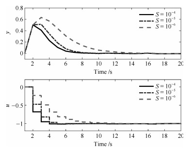
    图  5  $S$对系统抗扰能力的影响(输入扰动模型+输入扰动)

    Fig.  5  Disturbance rejection performance with different $S$ (input disturbance model + input disturbance)

    图  6  动态跟踪问题中的各种滞后

    Fig.  6  Lags in the tracking control problem

  • [1] 席裕庚, 李德伟, 林姝.模型预测控制—现状与挑战.自动化学报, 2013, 39(3): 222-236 doi: 10.3724/SP.J.1004.2013.00222

    Xi Yu-Geng, Li De-Wei, Lin Shu. Model predictive control—status and challenges. Acta Automatica Sinica, 2013, 39(3): 222-236 doi: 10.3724/SP.J.1004.2013.00222
    [2] Shinskey F G. Feedback Controllers for the Process Industries. New York: McGraw-Hill Professional, 1994. 117-119
    [3] Lundström P, Lee J H, Morari M, Skogestad S. Limitations of dynamic matrix control. Computers & Chemical Engineering, 1995, 19(4): 409-421 http://cn.bing.com/academic/profile?id=f784b1919df2f28bf79ef45d9c4c572f&encoded=0&v=paper_preview&mkt=zh-cn
    [4] Muske K R, Badgwell T A. Disturbance modeling for offset-free linear model predictive control. Journal of Process Control, 2002, 12(5): 617-632 http://www.wanfangdata.com.cn/details/detail.do?_type=perio&id=a53bce47218139e3782ace29d6d5a1bf
    [5] Aström K J, Hägglund T. PID Controllers: Theory, Design and Tuning (Second edition). USA: Instrument Society of America, 1995. 80-92
    [6] Garcia C E, Morari M. Internal model control. A unifying review and some new results. Industrial & Engineering Chemistry Process Design & Development, 1982, 21(2): 308-323 doi: 10.1021-i200017a016/
    [7] Morari M, Zafiriou E. Robust Process Control. Englewood Cliffs, NJ: Prentice-Hall, 1989.
    [8] 席裕庚.预测控制.第2版.北京:国防工业出版社, 2013

    Xi Yu-Geng. Predictive Control (Second edition). Beijing: National Defense Industry Press, 2013.
    [9] Maeder U, Morari M. Offset-free reference tracking with model predictive control. Automatica, 2010, 46(9): 1469-1476 http://www.wanfangdata.com.cn/details/detail.do?_type=perio&id=82a599115d96619621990f520aa8e59a
    [10] Young P C, Willems J C. An approach to the linear multivariable servomechanism problem. International Journal of Control, 1972, 15(5): 961-979 doi: 10.1080/00207177208932211
    [11] Franklin G F, Powell J D, Workman M L. Digital Control of Dynamic Systems (Third edition). Menlo Park, CA: Addison Wesley Longman Publishing Co., Inc., 1998. 322-336
    [12] Johnson C D. Accomodation of external disturbances in linear regulator and servomechanism problems. IEEE Transactions on Automatic Control, 1971, 16(6): 635-644 doi: 10.1109/TAC.1971.1099830
    [13] Davison E J, Smith H W. Pole assignment in linear time-invariant multivariable systems with constant disturbances. Automatica, 1971, 7(4): 489-498 doi: 10.1016/0005-1098(71)90099-9
    [14] Kwakernaak H, Sivan R. Linear Optimal Control Systems. New York: John Wiley & Sons, Inc., 1972. 278-279
    [15] Richalet J, Rault A, Testud J L, Papon J. Model predictive heuristic control: applications to industrial processes. Automatica, 1978, 14(5): 413-428 doi: 10.1016-0005-1098(78)90001-8/
    [16] Cutler C R, Ramaker B L. Dynamic matrix control: a computer control algorithm. In: Proceedings of the 1980 Joint Automatic Control Conference. San Francisco, USA, 1980.
    [17] Garcia C E, Morshedi A M. Quadratic programming solution of dynamic matrix control (QDMC). Chemical Engineering Communications, 1986, 46(1-3): 73-87 doi: 10.1080/00986448608911397
    [18] Clarke D W, Mohtadi C. Properties of generalized predictive control. Automatica, 1989, 25(6): 859-875 doi: 10.1016/0005-1098(89)90053-8
    [19] Marquis P, Broustail J. SMOC, a bridge between state space and model predictive controllers: application to the automation of a hydrotreating unit. IFAC Proceedings Volumes, 1988, 21(4): 37-45 doi: 10.1016/B978-0-08-035735-5.50010-3
    [20] Rawlings J B. Tutorial overview of model predictive control. IEEE Control Systems, 2000, 20(3): 38-52 http://cn.bing.com/academic/profile?id=80dc0712a8ee58d18b9749b8224d9743&encoded=0&v=paper_preview&mkt=zh-cn
    [21] Li S F, Lim K Y, Fisher D G. A state space formulation for model predictive control. AIChE Journal, 1989, 35(2): 241-249 doi: 10.1002/aic.690350208
    [22] Ricker N L. Model predictive control with state estimation. Industrial & Engineering Chemistry Research, 1990, 29(3): 374-382 http://d.old.wanfangdata.com.cn/OAPaper/oai_doaj-articles_af2ad960e2e7be4856a2fd53c7dba86d
    [23] Kwon W H, Byun D G. Receding horizon tracking control as a predictive control and its stability properties. International Journal of Control, 1989, 50(5): 1807-1824 doi: 10.1080/00207178908953467
    [24] Rawlings J B, Muske K R. The stability of constrained receding horizon control. IEEE Transactions on Automatic Control, 1993, 38(10): 1512-1516 doi: 10.1109/9.241565
    [25] Muske K R, Rawlings J B. Model predictive control with linear models. AIChE Journal, 1993, 39(2): 262-287 doi: 10.1002/aic.690390208
    [26] Lee J H, Morari M, Garcia C E. State-space interpretation of model predictive control. Automatica, 1994, 30(4): 707-717 doi: 10.1016/0005-1098(94)90159-7
    [27] Wang L P. A tutorial on model predictive control: using a linear velocity-form model. Developments in Chemical Engineering & Mineral Processing, 2004, 12(5-6): 573-614 http://cn.bing.com/academic/profile?id=57d01df231d6ee94633e98e901047a90&encoded=0&v=paper_preview&mkt=zh-cn
    [28] Froisy J B. Model predictive control—building a bridge between theory and practice. Computers & Chemical Engineering, 2006, 30(10-12): 1426-1435 https://academic.oup.com/her/article/15/2/125/550414
    [29] Morari M, Maeder U. Nonlinear offset-free model predictive control. Automatica, 2012, 48(9): 2059-2067 doi: 10.1016/j.automatica.2012.06.038
    [30] Akesson J, Hagander P. Integral action — a disturbance observer approach. In: Proceedings of the 2003 European Control Conference (ECC). Cambridge, UK: IEEE, 2015. 2577-2582
    [31] Rao C V, Wright S J, Rawlings J B. Application of interior-point methods to model predictive control. Journal of Optimization Theory & Applications, 1998, 99(3): 723-757 http://cn.bing.com/academic/profile?id=37dc2572a182e4eb56569ba6ef573176&encoded=0&v=paper_preview&mkt=zh-cn
    [32] Prett D M, García C E. Fundamental Process Control. Stoneham, MA: Butterworths, 1988
    [33] Betti G, Farina M, Scattolini R. A robust MPC algorithm for offset-free tracking of constant reference signals. IEEE Transactions on Automatic Control, 2013, 58(9): 2394-2400 doi: 10.1109/TAC.2013.2254011
    [34] Maciejowski J M. Predictive Control with Constraints. Englewood Cliffs: Prentice-Hall, 2002
    [35] González A H, Adam E J, Marchetti J L. Conditions for offset elimination in state space receding horizon controllers: a tutorial analysis. Chemical Engineering & Processing: Process Intensification, 2008, 47(12): 2184-2194 http://cn.bing.com/academic/profile?id=b39d1d783d51ed52a7998aacb43bc963&encoded=0&v=paper_preview&mkt=zh-cn
    [36] Betti G, Farina M, Scattolini R. An MPC algorithm for offset-free tracking of constant reference signals. In: Proceedings of the 51st IEEE Conference on Decision and Control. Maui, HI, USA: IEEE, 2012. 5182-5187
    [37] Tatjewski P. Advanced Control of Industrial Processes. London: Springer Verlag, 2007. 176-197
    [38] Tatjewski P. Disturbance modeling and state estimation for offset-free predictive control with state-space process models. International Journal of Applied Mathematics & Computer Science, 2014, 24(2): 313-323 http://cn.bing.com/academic/profile?id=6e8857562a4802d30d390cba6f9aed9c&encoded=0&v=paper_preview&mkt=zh-cn
    [39] Zou T. Offset-free strategy by double-layered linear model predictive control. Journal of Applied Mathematics, 2012, 2012: Article ID 808327
    [40] 吴明光, 钱积新.基于多目标分层的预测控制定态优化技术.化工学报, 2005, 56(1): 105-109 doi: 10.3321/j.issn:0438-1157.2005.01.019

    Wu Ming-Guang, Qian Ji-Xin. Multi-objective and layered steady-state optimization method of model predictive control. Journal of Chemical Industry and Engineering, 2005, 56(1): 105-109 doi: 10.3321/j.issn:0438-1157.2005.01.019
    [41] 邹涛, 丁宝苍, 张瑞.模型预测控制工程应用导论.北京:化学工业出版社, 2010.

    Zou Tao, Ding Bao-Cang, Zhang Rui. MPC: an Introduction to Industrial Applications. Beijing: Chemical Industry Press, 2010.
    [42] Rawlings J B, Amrit R. Optimizing process economic performance using model predictive control. In: Proceedings of the 2009 Nonlinear Model Predictive Control. Lecture Notes in Control & Information Sciences. Berlin, Heidelberg: Springer, 2009, 384: 119-138
    [43] Rao C V, Rawlings J B. Steady states and constraints in model predictive control. AIChE Journal, 1999, 45(6): 1266-1278 doi: 10.1002/aic.690450612
    [44] 丁宝苍.工业预测控制.北京:机械工业出版社, 2016.

    Ding Bao-Cang. Industrial Predictive Control. Beijing: China Machine Press, 2016.
    [45] Rajamani M R, Rawlings J B, Qin S J. Achieving state estimation equivalence for misassigned disturbances in offset-free model predictive control. AIChE Journal, 2009, 55(2): 396-407 doi: 10.1002/aic.11673
    [46] Badgwell T A, Muske K R. Disturbance model design for linear model predictive control. In: Proceedings of the 2002 American Control Conference. Anchorage, USA: IEEE, 2002. 1621-1625
    [47] Pannocchia G, Rawlings J B. Disturbance models for offset-free model predictive control. AIChE Journal, 2003, 49(2): 426-437 doi: 10.1002/aic.690490213
    [48] Maeder U, Borrelli F, Morari M. Linear offset-free model predictive control. Automatica, 2009, 45(10): 2214-2222 doi: 10.1016/j.automatica.2009.06.005
    [49] Pannocchia G. Offset-free tracking MPC: a tutorial review and comparison of different formulations. In: Proceedings of the 2015 European Control Conference. Linz, Austria: IEEE, 2015. 527-532
    [50] Wang H K, Xu Z H, Zhao J, Jiang A P. An optimal filter based MPC for systems with arbitrary disturbances. Chinese Journal of Chemical Engineering, 2017, 25(5): 632-640 doi: 10.1016/j.cjche.2016.09.011
    [51] Wang H K, Zhao J, Xu Z H, Shao Z J. Input and state estimation for linear systems with a rank-deficient direct feedthrough matrix. ISA Transactions, 2015, 57: 57-62 doi: 10.1016/j.isatra.2015.02.005
    [52] Aström K J. Introduction to Stochastic Control Theory. London: Academic Press, 1970.
    [53] Davison E J. The output control of linear time-invariant multivariable systems with unmeasurable arbitrary disturbances. IEEE Transactions on Automatic Control, 1972, 17(5): 621-630 doi: 10.1109/TAC.1972.1100084
    [54] Davison E J, Smith H W. A note on the design of industrial regulators: integral feedback and feedforward controllers. Automatica, 1974, 10(3): 329-332 doi: 10.1016/0005-1098(74)90044-2
    [55] Francis B A, Wonham W M. The internal model principle of control theory. Automatica, 1976, 12(5): 457-465 doi: 10.1016/0005-1098(76)90006-6
    [56] Rawlings J B, Mayne D Q. Model Predictive Control: Theory and Design. Boston, MA, USA: Addison-Wesley Longman Publishing Co., Inc., 2006.
    [57] Geromel J C, Bernussou J, Garcia G. $H_2$ and $H{_\infty}$ robust filtering for discrete-time linear systems. SIAM Journal on Control & Optimization, 2000, 38(5): 1353-1368
    [58] Speyer J L, Chung W H. Stochastic Processes, Estimation, and Control. Philadelphia: Society for Industrial and Applied Mathematics, 2008
    [59] Box G P, Jenkins G M. Time Series Analysis: Forecasting and Control. San Francisco, CA, USA: Holden-Day, 1970
    [60] Brockwell P J, Davis R A. Time Series: Theory and Methods. New York, USA: Springer-Verlag, 1987
    [61] Odelson B J, Rajamani M R, Rawlings J B. A new autocovariance least-squares method for estimating noise covariances. Automatica, 2006, 42(2): 303-308 doi: 10.1016/j.automatica.2005.09.006
    [62] Lima F V, Rajamani M R, Soderstrom T A, et al. Covariance and state estimation of weakly observable systems: application to polymerization processes. IEEE Transactions on Control Systems Technology, 2013, 42(4): 1249-1257. http://cn.bing.com/academic/profile?id=53a79c0373636eafc52382190236fc75&encoded=0&v=paper_preview&mkt=zh-cn
    [63] Rajamani M R, Rawlings J B. Estimation of the disturbance structure from data using semidefinite programming and optimal weighting. Automatica, 2009, 45(1): 142-148 doi: 10.1016/j.automatica.2008.05.032
    [64] Wang H K, Zhao J, Xu Z H, Shao Z J. Linear offset-free model predictive control: a minimum-variance unbiased filter based approach. In: Proceedings of the 52nd IEEE Conference on Decision and Control. Florence, Italy: IEEE, 2013. 782-786
    [65] Shead L R E, Muske K R, Rossiter J A. Conditions for which linear MPC converges to the correct target. Journal of Process Control, 2010, 20(10): 1243-1251 doi: 10.1016/j.jprocont.2010.09.001
    [66] Davison E J. The robust control of a servomechanism problem for linear time-invariant multivariable systems. IEEE Transactions on Automatic Control, 1976, 21(1): 25-34 doi: 10.1109/TAC.1976.1101137
    [67] Johnson C. Further study of the linear regulator with disturbances—the case of vector disturbances satisfying a linear differential equation. IEEE Transactions on Automatic Control, 1970, 15(2): 222-228 doi: 10.1109/TAC.1970.1099406
    [68] Wonham W M. Tracking and regulation in linear multivariable systems. SIAM Journal on Control, 1973, 11(3): 424-437 doi: 10.1137/0311035
    [69] Wonham W M, Pearson J B. Regulation and internal stabilization in linear multivariable systems. SIAM Journal on Control, 1974, 12(1): 5-18 doi: 10.1137/0312002
    [70] Pearson J, Shields R, Staats P. Robust solutions to linear multivariable control problems. IEEE Transactions on Automatic Control, 1974, 19(5): 508-517 doi: 10.1109/TAC.1974.1100679
    [71] Francis B, Sebakhy O A, Wonham W M. Synthesis of multivariable regulators: the internal model principle. Applied Mathematics and Optimization, 1974, 1(1): 64-86 http://cn.bing.com/academic/profile?id=58970e1b229940be8283923ba7e068cf&encoded=0&v=paper_preview&mkt=zh-cn
    [72] Qin S J, Badgwell T A. A survey of industrial model predictive control technology. Control Engineering Practice, 2003, 11(7): 733-764 doi: 10.1016/S0967-0661(02)00186-7
    [73] Pannocchia G, Bemporad A. Combined design of disturbance model and observer for offset-free model predictive control. IEEE Transactions on Automatic Control, 2007, 52(6): 1048-1053 doi: 10.1109/TAC.2007.899096
    [74] 王浩坤.无偏模型预测控制的若干理论和方法研究[博士学位论文], 浙江大学, 中国, 2015 http://cdmd.cnki.com.cn/Article/CDMD-10335-1015305300.htm

    Wang Hao-Kun. Theories and Methods for Offset-Free Model Predictive Control [Ph. D. dissertation], Zhejiang University, China, 2015 http://cdmd.cnki.com.cn/Article/CDMD-10335-1015305300.htm
    [75] 钱积新, 赵均, 徐祖华.预测控制.北京:化学工业出版社, 2007.

    Qian Ji-Xin, Zhao Jun, Xu Zu-Hua. Predictive Control. Beijing: Chemical Industry Press, 2007.
    [76] Sun Z J, Zhao Y, Qin S J. Improving industrial MPC performance with data-driven disturbance modeling. In: Proceedings of the 50th IEEE Conference on Decision and Control and European Control Conference. Orlando, USA: IEEE, 2011. 1922-1927
    [77] Pannocchia G. Robust model predictive control with guaranteed setpoint tracking. Journal of Process Control, 2004, 14(8): 927-937 doi: 10.1016/j.jprocont.2004.03.001
    [78] Äström K J, Wittenmark B. Computer-Controlled Systems: Theory and Design, (Third edition). Englewood Cliffs, N.J.: Prentice Hall, 1996.
    [79] 钱积新.控制理论研究中的几个挑战性的问题.控制工程, 2005, 12(3): 193-195 doi: 10.3969/j.issn.1671-7848.2005.03.001

    Qian Ji-Xin. Some challenging problems in research on control theory. Control Engineering of China, 2005, 12(3): 193-195 doi: 10.3969/j.issn.1671-7848.2005.03.001
    [80] Hovd M. Improved target calculation for model predictive control. Modeling, Identification and Control, 2007, 28(3): 81-86 doi: 10.4173/mic.2007.3.3
    [81] Rawlings J B, Bonne D, Jorgensen J B, Venkat A N, Jorgensen S B. Unreachable setpoints in model predictive control. IEEE Transactions on Automatic Control, 2008, 53(9): 2209-2215 doi: 10.1109/TAC.2008.928125
    [82] Limon D, Alvarado I, Alamo T, Camacho E F. MPC for tracking piecewise constant references for constrained linear systems. Automatica, 2008, 44(9): 2382-2387 doi: 10.1016/j.automatica.2008.01.023
    [83] Gilbert E G, Kolmanovsky I, Tan K T. Discrete-time reference governors and the nonlinear control of systems with state and control constraints. International Journal of Robust and Nonlinear Control, 1995, 5(5): 487-504 doi: 10.1002/rnc.4590050508
    [84] Rossiter J A, Kouvaritakis B, Gossner J R. Feasibility and stability results for constrained stable generalized predictive control. Automatica, 1995, 31(6): 863-877 doi: 10.1016/0005-1098(94)00166-G
    [85] Bemporad A, Casavola A, Mosca E. Nonlinear control of constrained linear systems via predictive reference management. IEEE Transactions on Automatic Control, 1997, 42(3): 340-349 doi: 10.1109/9.557577
    [86] Wang H K, Zhao J, Xu Z H, Shao Z J. Model predictive control for Hammerstein systems with unknown input nonlinearities. Industrial & Engineering Chemistry Research, 2014, 53(18): 7714-7722 http://www.wanfangdata.com.cn/details/detail.do?_type=perio&id=f7559988503aab59e5d0d19aabf9e767
    [87] Wang H K, Jiang A P. An active fault-tolerant MPC for systems with partial actuator failures. In: Proceedings of the 11th Asian Control Conference. Gold Coast, Australia: IEEE, 2017. 1614-1619
    [88] Lima F V, Rawlings J B. Nonlinear stochastic modeling to improve state estimation in process monitoring and control. AIChE Journal, 2011, 57(4): 996-1007 doi: 10.1002/aic.12308
    [89] Zagrobelny M A, Rawlings J B. Practical improvements to autocovariance least-squares. AIChE Journal, 2015, 61(6): 1840-1855 doi: 10.1002/aic.14771
    [90] Mehra R. Approaches to adaptive filtering. IEEE Transactions on Automatic Control, 1972, 17(5): 693-698 doi: 10.1109/TAC.1972.1100100
    [91] Mehra R. On the identification of variances and adaptive Kalman filtering. IEEE Transactions on Automatic Control, 1970, 15(2): 175-184 doi: 10.1109/TAC.1970.1099422
    [92] Myers K, Tapley B. Adaptive sequential estimation with unknown noise statistics. IEEE Transactions on Automatic Control, 1976, 21(4): 520-523 doi: 10.1109/TAC.1976.1101260
    [93] Bodizs L, Srinivasan B, Bonvin D. On the design of integral observers for unbiased output estimation in the presence of uncertainty. Journal of Process Control, 2011, 21(3): 379-390 doi: 10.1016/j.jprocont.2010.11.015
    [94] 陈虹.模型预测控制.北京:科学出版社, 2013.

    Chen Hong. Model Predictive Control. Beijing: Science Press, 2013.
    [95] Mohammadkhani M, Bayat F, Jalali A A. Two-stage observer based offset-free MPC. ISA Transactions, 2015, 57: 136-143 doi: 10.1016/j.isatra.2015.02.015
    [96] Mayne D Q. Model predictive control: recent developments and future promise. Automatica, 2014, 50(12): 2967-2986 doi: 10.1016/j.automatica.2014.10.128
    [97] Pannocchia G, Kerrigan E C. Offset-free receding horizon control of constrained linear systems. AIChE Journal, 2005, 51(12): 3134-3146 doi: 10.1002/aic.10626
    [98] Ding B C, Zou T, Pan H G. A discussion on stability of offset-free linear model predictive control. In: Proceedings of the 24th Chinese Control and Decision Conference. Taiyuan, China: IEEE, 2012. 80-85
    [99] Kassmann D E, Badgwell T A, Hawkins R B. Robust steady-state target calculation for model predictive control. AIChE Journal, 2000, 46(5): 1007-1024 doi: 10.1002/aic.690460513
    [100] Seborg D E, Edgar T F, Mellichamp D A. Process Dynamics and Control (Second edition). New York: John Wiley & Sons, Inc., 2004.
    [101] Tatjewski P. Advanced control and on-line process optimization in multilayer structures. Annual Reviews in Control, 2008, 32(1): 71-85 doi: 10.1016/j.arcontrol.2008.03.003
    [102] Darby M L, Nikolaou M, Jones J, Nicholson D. RTO: an overview and assessment of current practice. Journal of Process Control, 2011, 21(6): 874-884 doi: 10.1016/j.jprocont.2011.03.009
    [103] Würth L, Hannemann R, Marquardt W. A two-layer architecture for economically optimal process control and operation. Journal of Process Control, 2011, 21(3): 311-321 doi: 10.1016/j.jprocont.2010.12.008
    [104] Zanin A C, Tvrzská de Gouvêa M, Odloak D. Integrating real-time optimization into the model predictive controller of the FCC system. Control Engineering Practice, 2002, 10(8): 819-831 doi: 10.1016/S0967-0661(02)00033-3
    [105] Adetola V, Guay M. Integration of real-time optimization and model predictive control. Journal of Process Control, 2010, 20(2): 125-133 doi: 10.1016/j.jprocont.2009.09.001
    [106] Alvarez L A, Odloak D. Robust integration of real time optimization with linear model predictive control. Computers & Chemical Engineering, 2010, 34(12): 1937-1944 doi: 10.1016-j.compchemeng.2010.06.017/
    [107] Helbig A, Abel O, Marquardt W. Structural concepts for optimization based control of transient processes. In: Nonlinear Model Predictive Control. Progress in Systems and Control Theory. Basel: Birkhäuser Verlag, 2000. 295-311
    [108] Morari M, Arkun Y, Stephanopoulos G. Studies in the synthesis of control structures for chemical processes: Part Ⅰ: Formulation of the problem. Process decomposition and the classification of the control tasks. Analysis of the optimizing control structures. AIChE Journal, 1980, 26(2): 220-232 doi: 10.1002/aic.690260205
    [109] Pannocchia G, Gabiccini M, Artoni A. Offset-free MPC explained: novelties, subtleties, and applications. IFAC-PapersOnLine, 2015, 48(23): 342-351 doi: 10.1016/j.ifacol.2015.11.304
  • 期刊类型引用(13)

    1. 翟宇佳,陈锐勇,谢长勇,付国举,廖昌波. 基于模型预测控制的微压氧舱系统设计. 海军医学杂志. 2024(03): 319-322 . 百度学术
    2. 王华秋,朱天虎,高鹏. 分层表冷器的水循环优化预测控制研究. 控制工程. 2024(06): 1004-1011 . 百度学术
    3. 胡开成,严爱军,王殿辉. 城市固废焚烧过程炉温非线性模型预测控制. 控制理论与应用. 2024(11): 2023-2032 . 百度学术
    4. 张锴杨,徐逢秋,许贤泽. 约束不确定系统的误差有界无偏跟踪. 控制与决策. 2023(02): 450-458 . 百度学术
    5. 胡小勇,张建军,邓志刚,杨云晖. 基于迭代学习辨识算法的非线性宏观交通流参数优化. 现代电子技术. 2023(13): 183-186 . 百度学术
    6. 凌晓定,熊鑫,吴啸. 基于变步长预测控制的综合能源系统热电协调运行方法研究. 电站系统工程. 2023(05): 55-59 . 百度学术
    7. 汪磊,许锋,罗雄麟. 预测控制系统直接操纵流量调节阀阀位的控制性能评价. 化工自动化及仪表. 2022(04): 438-445 . 百度学术
    8. 罗震,罗怡沁,严伟鑫. 基于模型预测控制的飞机蒙皮铣削方法研究. 自动化仪表. 2022(07): 55-60+66 . 百度学术
    9. 张增吉,徐可心,叶飞. 多目标约束条件下基于MPC煤磨出口温度控制策略研究. 水泥工程. 2022(04): 63-64+87 . 百度学术
    10. 熊飞飞,黄景涛,茅建波. 一种自适应阶梯式广义预测控制方法. 控制工程. 2022(11): 2145-2151 . 百度学术
    11. 吴建范,蒙艳玫,柳宏耀. 基于核极限学习机的煮糖结晶自适应控制研究. 广西科学. 2021(03): 249-256 . 百度学术
    12. 邵明明,刘友波,陈婧婷,王潇笛,左坤雨,刘俊勇. 分散式储能自趋优经济运行的强化学习算法. 电网技术. 2020(05): 1696-1705 . 百度学术
    13. 李璐,刘远,周宇航. 永磁同步电机鲁棒模型预测控制技术综述. 工业仪表与自动化装置. 2020(05): 11-15 . 百度学术

    其他类型引用(39)

  • 加载中
  • 图(6)
    计量
    • 文章访问数:  3041
    • HTML全文浏览量:  1394
    • PDF下载量:  951
    • 被引次数: 52
    出版历程
    • 收稿日期:  2018-06-12
    • 录用日期:  2018-09-17
    • 刊出日期:  2020-06-01

    目录

    /

    返回文章
    返回