2.845

2023影响因子

(CJCR)

  • 中文核心
  • EI
  • 中国科技核心
  • Scopus
  • CSCD
  • 英国科学文摘

留言板

尊敬的读者、作者、审稿人, 关于本刊的投稿、审稿、编辑和出版的任何问题, 您可以本页添加留言。我们将尽快给您答复。谢谢您的支持!

姓名
邮箱
手机号码
标题
留言内容
验证码

目标跟踪算法综述

孟琭 杨旭

孟琭, 杨旭. 目标跟踪算法综述. 自动化学报, 2019, 45(7): 1244-1260. doi: 10.16383/j.aas.c180277
引用本文: 孟琭, 杨旭. 目标跟踪算法综述. 自动化学报, 2019, 45(7): 1244-1260. doi: 10.16383/j.aas.c180277
MENG Lu, YANG Xu. A Survey of Object Tracking Algorithms. ACTA AUTOMATICA SINICA, 2019, 45(7): 1244-1260. doi: 10.16383/j.aas.c180277
Citation: MENG Lu, YANG Xu. A Survey of Object Tracking Algorithms. ACTA AUTOMATICA SINICA, 2019, 45(7): 1244-1260. doi: 10.16383/j.aas.c180277

目标跟踪算法综述

doi: 10.16383/j.aas.c180277
基金项目: 

国家自然科学基金 61101057

详细信息
    作者简介:

    杨旭  东北大学信息科学与工程学院硕士研究生.主要研究方向为图像处理.E-mail:13998346746@163.com

    通讯作者:

    孟琭  东北大学信息科学与工程学院副教授.主要研究方向为人工智能及图像处理.本文通信作者. E-mail:menglu@ise.neu.edu.cn

A Survey of Object Tracking Algorithms

Funds: 

National Natural Science Foundation of China 61101057

More Information
    Author Bio:

     Master student at the College of Information Science and Engineering, Northeastern University. His main research interest is image processing

    Corresponding author: MENG Lu  Associate professor at the College of Information Science and Engineering, Northeastern Universiy. His research interest covers artificial intelligence and image processing. Corresponding author of this paper
  • 摘要: 目标跟踪一直以来都是计算机视觉领域的关键问题,最近随着人工智能技术的飞速发展,运动目标跟踪问题得到了越来越多的关注.本文对主流目标跟踪算法进行了综述,首先,介绍了目标跟踪中常见的问题,并由时间顺序对目标跟踪算法进行了分类:早期的经典跟踪算法、基于核相关滤波的跟踪算法以及基于深度学习的跟踪算法.接下来,对每一类中经典的跟踪算法的原始版本和各种改进版本做了介绍、分析以及比较.最后,使用OTB-2013数据集对目标跟踪算法进行测试,并对结果进行分析,得出了以下结论:1)相比于光流法、Kalman、Meanshift等传统算法,相关滤波类算法跟踪速度更快,深度学习类方法精度高.2)具有多特征融合以及深度特征的追踪器在跟踪精度方面的效果更好.3)使用强大的分类器是实现良好跟踪的基础.4)尺度的自适应以及模型的更新机制也影响着跟踪的精度.
  • 大多数的工程和科学应用, 如工业制造、城市运输、污水处理和资本运算等, 几乎每个重要的现实生活中的决策都存在多目标优化问题.这些目标往往是不可比较, 甚至是相互冲突的.因此多目标优化问题(Multiobjective optimization problem, MOP)一直是近几年主要的研究课题之一.为了解决该问题, 多目标进化算法(Multiobjective evolutionary algorithm, MOEAs)已被广泛研究.其中Schaffer[1]提出了向量评估遗传算法(Vector evaluated genetic algorithm, VE-GA), 该算法对单目标遗传算法进行了改进.但VEGA只能找到Pareto前端的始末端, 产生不了均匀分布的解.为此Fonseca等[2]提出了多目标遗传算法(Multiobjective genetic algorithm, MOGA), 这种算法效率较高, 而且易于实现.但该算法的不足在于如果小生境数目信息是基于目标函数的, 那么两个具有相同目标函数向量的不同个体无法在同一代种群中存在.为了解决该问题, Srinivas等[3]提出了非劣分类遗传算法(Nondominated sorting genetic algorithm, NSGA), 该算法先按解个体的非劣关系进行排序, 再按照共享机制来保持进化的多样性.但是该算法计算效率较低, 计算复杂度大, 且共享参数$ \sigma $需要预先确定.为了减小算法的计算复杂度, Deb等[4]提出了改进型非劣分类遗传算法(Nondominated sorting genetic algorithm Ⅱ, NSGAII), 该算法采用非支配排序进行分级, 通过计算拥挤距离选择最优解, 并将其做为精英解保存起来.但该算法是一种类随机搜索算法, 存在操作次数多收敛速度慢和解分布特性较差的问题[5].

    由于种群在迭代过程中种群分布不均会导致种群多样性变差从而易使解陷入局部最优, 并且在迭代过程中Pareto前沿部分区域易出现空白, 收敛速度变慢.为了解决种群分布不均带来的上述的问题, Goldberg等[6]提出了基于共享机制的小生境技术, 该方法考虑了一个个体与群体中其他个体之间的相似程度, 但计算开销比较大.朱学军等[7]提出用进化群体熵来刻画进化群体的多样性和分布性.然而这种方法缺乏对群体内部个体之间关系的刻画, 因此不便于调控群体进化过程中的多样性和分布性.为了解决这个问题, Corne等[8]提出了网格方法, 将网格中聚集密度大的个体删除, 但不能删除极点个体. Knowles等[9]提出了自适应网格技术, 在每一代进化时, 根据当前代的个体分布情况自适应地调整边界. Morse[10]提出了聚类分析的方法来保持种群的多样性. Han等[11]提出了基于种群间距信息和种群分布熵的方法.但是以上方法只能删除种群中拥挤距离较小的个体, 无法解决解的过程中Pareto前沿部分区域出现空白的问题.

    基于以上问题, 本文提出了一种基于均匀分布的NSGAII (NSGAII-UID)多目标优化算法.该算法受文献[12]的启发, 将种群映射到目标值对应的超平面上, 并在该平面上聚类.但是文献[12]中提出的算法仍然存在种群分布不均的问题, 从而影响了种群的多样性, 为了解决该问题, 本文将映射平面均匀分区.当对应区间的分布性不满足时, 分布性加强模块激活.由于种群在迭代的过程中对应区间会出现种群个体不足或缺失的状况, 此时需要在该区间内放入一些个体.为了解决该问题, 本文将所选聚类子群体中拥挤距离最大的点进行局部搜索, 采用极限优化变异[13]的方法产生新的个体.实验结果表明, 该方法综合评价指标(Inverted generational distance, IGD)值和分布性评价指标(Spacing, SP)值均高于其他算法.因此表明该方法具有较好的种群多样性和分布性, 且收敛速度较快.

    定义1.多目标优化问题(MOP)

    一个具有$ n $个决策变量, $ m $个目标函数的多目标优化问题可以描述为:

    $ \min {\pmb F({\pmb {X}})}=(f_{1} ({\pmb {X}}), \cdots, f_{j} ({\pmb {X}}), \cdots, f_{m} ({\pmb {X}})) $

    (1a)

    $ {\pmb x}=(x_{1}, x_{2}, \cdots, x_{n} )^{\rm T} \in {\pmb {X}}\subset {\bf R}^{n} $

    (1b)

    $ l_{i} \leq x_{i} \leq u_{i}, \quad i=1, 2, \cdots, n $

    (1c)

    式中, ${\pmb x}$称为决策变量, $ {\pmb {X}} $是$ n $维的决策空间; $ {\pmb F({\pmb {X}})}\in {\bf R}^{m} $为$ m $维目标向量; $ f_{j}({\pmb {X}}) (j= 1, 2$, $ \cdots, m) $为第$ j $个目标函数, $ l_{i} $和$ u_{i} $分别为第$ i $个决策变量的上界和下界.

    定义2. Pareto-占优对于给定的两点$ x $, $ x^{*}\in X_{f} $, $ x^{*} $是Pareto-占优(非支配)的, 当且仅当式(2)成立, 记为$ x^{*} > x $.

    $ (\forall\: i\in \{1, 2, \cdots, m\}: f_{i} (x^{\ast })\leq f_{i} (x)) $

    (2a)

    $ \wedge (\exists\: k\in \{1, 2, \cdots, m\}: f_{k} (x^{\ast })\leq f_{k} (x)) $

    (2b)

    定义3. Pareto-最优解

    若对于任意解$ x $, 不存在$ x'\in \Omega $使得, $ f_{2}(x^{\prime}), \cdots, f_{m}(x^{\prime})) $占优于$ {\pmb F(x)} =(f_{1}(x) $, $ f_{2}(x), \cdots, f_{m}(x)) $, 则称$ x $为Pareto最优解或者非劣解.

    定义4. Pareto-最优解集

    所有Pareto-最优解组成的集合$ P_{s} $称为Pareto-最优解集.

    定义5. Pareto-前沿

    Pareto-最优解集合$ {{P}}_{s} $中的解对应的目标函数值组成的集合$ {{P}}_{F} $称为Pareto-前沿, 即:

    $ \begin{equation} \label{eq6} {{P}}_{F} =\{{\pmb F(x)}=(f_{1} (x), f_{2} (x), \cdots, f_{m} (x))|x\in P_{s} \} \end{equation} $

    (3)

    设$ n $个数据样本为, $ c ({2} \leq c\leq n) $是要将数据样本分成不同类型的数目, 表示相应的$ C $个类别, 是其相似分类矩阵, 各类别的聚类中心为$ \{ v_{1}, v_{2}, \cdots, v_{n} \} $, $ \mu _{k} (p_{i}) $是样本$ p_{i} $对于类$ A_{k} $的隶属度(简写为$ \mu _{k}) $.则目标函数$ J_{b} $可以表达为:

    $ \begin{equation} \label{eq7} J_{b} ({{P}}, v)=\sum\limits_{i=1}^n {\sum\limits_{k=1}^c {(\mu_{ik} )^{b}(d_{ik} )^{2}} } \end{equation} $

    (4)

    $ \begin{equation} \label{eq8} d_{ik} =d(p_{i} -v_{k} )=\sqrt{\sum\limits_{j=1}^m {(p_{_{ij} } -v_{_{kj} } )^{2}} } \end{equation} $

    (5)

    其中, $ d_{ik} $是欧几里得距离, 用来度量第$ i $个样本$ p_{i} $与第$ k $类中心点之间的距离; $ m $是样本的特征数; $ b $是加权参数, 取值范围是$ 1 \leq b\leq \infty $.模糊$ C $-均值聚类方法就是寻找一种最佳的分类, 以使该分类能产生最小的函数值$ J_{b} $.它要求一个样本对于各个聚类的隶属度值和为1, 即满足:

    $ \sum\limits_{j=1}^c {\mu_{j} (p_{i} )} =1, \quad i=1, 2, \cdots, n $

    (6a)

    $ \mu_{ik} =\dfrac{1}{\sum\limits_{j=1}^c {\left(\dfrac{d_{ik} }{d_{_{lk} } }\right)^{\frac{2}{b-1}}} } $

    (6b)

    $ v_{ij} =\frac{\sum\limits_{k=1}^n {(\mu_{_{ik} } )^{n}p_{_{kj} } } }{\sum\limits_{k=1}^n {(\mu_{_{ik} } )^{b}} } $

    (6c)

    设$ I_{k} =\{i | 2 \leq c < n $; $ d_{ik}= 0 \} $, 对于所有的$ i $类, $ i\in I_{k} $, $ \mu _{ik}= 0 $.当算法收敛时, 理论上就得到了各类的聚类中心以及各个样本对于各模式类的隶属度, 从而完成了模糊聚类划分.

    为了解决种群分布不均的问题, 本文提出了将目标空间均匀分区, 选取相同数量个体的方法.由于目标空间一般为曲线或者曲面, 想要均匀划分较难操作.为了解决这个问题, 本文受文献[12]的启发, 在文献[12]中, 种群中的个体映射在一个超平面上, 并在目标空间中聚类.为了验证种群的多样性将集群质量度量标准.但是该方法在迭代过程中存在种群分布不均的问题, 从而影响种群的多样性, 进而造成收敛速度慢, Pareto前沿有些区域出现空白的现象.针对以上问题本文提出了将种群映射到目标函数值对应的超平面$ H $, 在$ H $上进行均匀分区以增加种群的多样性的方法.该方法将种群在映射平面上进行聚类, 并记录聚类中心, 计算每个分区中的聚类中心个数, 从而判断是否满足均匀分布条件.当条件不满足时, 分布性加强模块激活.由于在计算过程中区间内有时会出现个体数量不足或者为空的情况, 为了在该区间获取缺失的个体, 本文采用极限优化变异产生新的个体.当该区间个体不为空时, 将聚类子群体按照拥挤距离从大到小排序, 选取第一个个体进行变异.当该区域为空时, 将离该区间最近的个体进行变异.该方法不但可以使种群跳出局部最优, 并且能够较快地找到Pareto前端.

    设目标向量为:

    $ \begin{equation} \label{eq12} {\pmb A}^{i}=(0, \cdots, 0, a_{i}^{\max }, 0, \cdots, 0)^{\rm T}\in {\bf R}^{k} \end{equation} $

    (7)

    $ a_{i}^{\max} $为种群$ P $中目标向量$ a_{i} $的最大函数值.

    $ a_{i}^{\max } \in {\bf R}\backslash 0, \qquad i=1, 2, \cdots, k $

    (8)

    定义超平面[12] $H$为$ k $维欧氏空间的$ k -1 $维线性子空间, $ b^{s}= - 1 $, $ \langle\cdot \rangle $为欧氏内积

    $ \begin{equation} \label{eq9} H=\left\{ {a\in {\bf R}^{k}: \left\langle {{\pmb W}^{s}, f} \right\rangle +b^{s}=0} \right\} \end{equation} $

    (9)

    目标向量$ f $映射到超平面[12] $H $为$ {PI} $, 公式如下所示:

    $ {\pmb W}^{s}=\left(\frac{1}{f_{1}^{\max } }, \cdots, \frac{1}{f_{i}^{\max } }, \cdots, \frac{1}{f_{k}^{\max } }\right) $

    (10)

    $ PI=\frac{1-\left\langle {{\pmb W}^{s}, f} \right\rangle }{\left\| {{\pmb W}^{s}} \right\|^{2}} {\pmb W}^{s}+f $

    (11)

    映射到超平面的子群体为$ {RP} _{i}^{t} $, $ i= 1, 2, \cdots, K $, 其中$ K $为子群体的个数, 在公式中, 如果$ f_{i}^{\max }= 0 $, 则设置$ f_{i}^{\max }= 10^{-6} $.

    $ Q=\sum\limits_{i=1}^K {\frac{1}{\left| {RP_{i}^{t} } \right|}} \sum\nolimits_{C_{j} \in RP_{i}^{t} } {(D(C_{j}, \sigma_{i} ))} $

    (12)

    $ Q: $集群质量指数, $ | RP_{i}^{t} | $为聚类$ i $的个体数量, 为聚类中心, $ C_{j} $为聚类的一个点.

    由于NSGAII在运算过程中种群的分布性较差, 为了解决这个问题, 本文加入了分布性判断模块.该模块用来判断每个均匀分段区间内聚类子群体的分布情况, 同时选取聚类子群体中种类数量最大值作为阈值来判断分布性.当区间内种群类别小于该阈值时, 则判断该区间不满足分布性, 分布性加强模块激活.否则, 该区域满足分布性, 且选取每个聚类子群体中拥挤距离最大的个体放入精英档案.

    该算法首先将目标区间均匀分区, 其中每个区间的种群分布如下:

    $ \begin{equation} \label{eq13} {{D}}_{o} =\{D_{o1}, \cdots, D_{oi}, \cdots, D_{on} \} \end{equation} $

    (13)

    $ n $为分段区间的数量, $ D_{oi} $为第$ i $个区间所包含的子群体所有类别的集合, $ i\in [1, n] $, 如下所示:

    $ \begin{equation} \label{eq14} {{D}}_{on} =[{\pmb {NRP}}_{n1}, \cdots, {\pmb {NRP}}_{ij}, \cdots, {\pmb {NRP}}_{nr} ] \end{equation} $

    (14)

    $ \begin{equation} \label{eq15} {\pmb {NRP}}_{ij} =({{AB}}_{nr1}, \cdots, { {AB}}_{nrk}, \cdots, { {AB}}_{nrm} ) \end{equation} $

    (15)

    ${\pmb {NRP}}_{ij} $为第$ i $个区间内的种群中心编号, 其中$ i\in [1, n], j\in [1, r] $, $ r $为种群中心数量, 为第$ i $个区间第$ r $个聚类中心所对应的个体, $ k\in [1, m] $, $ m $为该类子群体个体数量.区间内种群中心数量最大值为$ {\max nr} $.判断种群分布性的方法如下所示:

    $ \begin{equation} \label{eq16} \begin{aligned} &ir < \max nr, \text{情况} 1 \\ &ir =\max { {D}}_{on}, \text{情况} 2 \\ \end{aligned} \end{equation} $

    (16)

    其中, $ {ir} $为第$ i $个区间内的种群中心数量, 为分段区间内种群中心数量最大值.

    情况1. 若该条件成立, 则分布性加强模块激活.

    情况2. 将该类子群体按照拥挤距离从大到小排序, 选择每个聚类子群体第一个个体.

    当种群不满足上述分布性条件时, 分布性加强模块被激活.在种群选取的过程中, 每个区间选择相同数量的个体.同时为了增加种群的多样性, 从每个聚类子群体中按照方法1)与2)选取拥挤距离较大的个体放入精英档案.然而在运算的过程中, 区间内有时会出现种群数量不足或空缺的状况.在以往文献中多是采用将拥挤距离较小的个体删除的方法, 当种群空缺或不足时, 并未有相关文献进行介绍.为了解决这个问题, 本文提出了对所选精英个体进行极限优化变异的方法, 来填补欠缺的个体.由于在计算过程中区间内种群中心的数量不同, 采取的策略也不相同.具体方法如下所示:

    1) 第$ i $个区间种群中心个数量$ ir $为0:

    $ \begin{equation}\label{eq17} \begin{cases} {icm\geq \max nr}, & \text{情况 1} \\ {icm < \max nr}, & \text{情况 2} \\ {icm=0}, & \text{情况 3} \\ \end{cases} \end{equation} $

    (17)

    其中$ icm $为在第$ i $个区间内第$ {c} $个聚类中心对应的子群体中的个体数量, $ {c} \in [1, ir] \cup 0. $

    情况1. 将该类子群体按照拥挤距离从大到小排序, 取前个个体.

    情况2. 选取所有个体, 剩余$ {\rm max}nr$-$icm $个个体由拥挤距离最大的个体变异得到. (详见第2.4节)

    情况3. 由于该区间无个体, 本文选取离该区间最近的两个个体变异得到$ {\rm max}nr $个个体(详见第2.4节).若该区间连续20次为空则该区间设定为空.

    2) 第$ i $个区间种群中心个数量$ ir $不为0:

    当该区间种群中心个数不为零时, 需要从聚类中心对应的子群体中选择相应的个体.选择方式如下所示:

    $ \begin{equation} \label{eq18} S\_num=floor({\rm max}nr/ir) \end{equation} $

    (18)

    $ \begin{equation} \label{eq19} |Re_{nr}| ={\rm max}nr-S\_num\times ir \end{equation} $

    (19)

    $ \begin{equation} \label{eq20} {\pmb {Re}}_{nr} =(Re_{nr1}, \cdots, Re_{nri}, \cdots, Re_{nrt} ) \end{equation} $

    (20)

    $ \textit{S_num}$为每个聚类子群体应当平均选择的个体数目, $ {\pmb {Re}}_{nr} $为需要选择的剩余个体的集合, $|Re_{nr}|$为需要选择的剩余个体的集合的数量, $Re _{nri} $为剩余的个体对应编号, $ i\in [1, t] $, $ t $为余数的个数.根据余数的是否为0, 选择方式也不相同, 具体如下:

    a) 余数$ {Re} _{r} $为0:

    $ \begin{equation} \label{eq21} \begin{cases} {icm\geq S\_num}, & \text{情况 1} \\ {icm < S\_num}, & \text{情况 2} \\ \end{cases} \end{equation} $

    (21)

    情况1. 将该类子群体按照拥挤距离排序, 取前$ \textit{S_num}$个个体.

    情况2. 选取所有个体, 剩$\textit{nrm}-\textit{S_num}$个个体由变异得到. (详见第2.4节)

    b) 余数${Re} _{r} $不为0:

    当剩余个体数量不为0时, 选择的方式如下所示:

    $ \begin{equation} \label{eq22} \begin{cases} {icm\geq S\_num+Re_{r} }, & \text{情况 1} \\ {icm < S\_num+Re_{r} }, & \text{情况 2} \\ \end{cases} \end{equation} $

    (22)

    情况1. 将该类子群体按照拥挤距离排序, 取前$ \textit{S_num}$个个体, 剩余$ {\pmb {Re}} _{nr} $个个体随机从第$\textit{rand} $$ (1, \textit{ir}) $个子群体选取.若$ \pmb{NRP}_{ij} $对应的子群体被选中$ k $次, 则从第$ \textit{S_num}$ $ + k +1 $个个体开始选取.

    情况2. 当$ \textit{icm} < \textit{S_num}$时, 选取全部个体, 剩余$\textit{S_num}-\textit{icm}$个个体由变异得到(详见第2.4节).当时, $ \pmb{NRP} _{ij} $对应的子群体选择前$ \textit{S_num}$个个体, 若该群体被选中$ k $次, 且$\textit{icm} >= \textit{S_num} + k $, 则从第$ \textit{S_num}$ $ +k +1 $个开始选取.若$ \textit{icm} < \textit{S_num} +k $, 则重新随机选择.

    由于在迭代过程中有的时候区间会出现种群数量不足或为空的状况.为了保证每个区间个体选取数量相同.本文采取最优个体极限优化变异策略.首先找到需要选择子群体中拥挤距离最大的个体或者离该区间最近的两个个体, 然后对其进行变异, 本文采用两种变异策略来产生局部解[13]:

    1) 第一种变异策略:

    对于选定的对象, 每次只有一个决策变

    量发生变异, 这样有效的提高了种群的局部搜索能力, 从而提高了解的计算精度.设当前选定个体, $ {j} $为决策变量的个数.种群总数为$N $, 则产生局部解的个数为$\mu, \mu $的值由上文(详见第2.3节)的需要动态决定.具体如下:

    $ \begin{gather}\label{eq23}\nonumber {\pmb {AB}}_{nrm} =(AB_{nrm1}, \cdots, AB_{nrmi}^{\prime}, \cdots, AB_{nrmj} )\\ 0 < i\leq j \end{gather} $

    (23)

    $ { {AB}}_{nrmi}^{\prime} \!=\!AB_{nrmi} \!+\!\delta \cdot \theta_{\max } (AB_{nrmi} ), \ 0 < i\leq j $

    (24)

    $ \delta = \begin{cases} (2\alpha )^{\frac{1}{1+\beta}}-1 \\ 1-\left[ {2(1-\alpha )} \right]^{\frac{1}{1+\beta}} \\ \end{cases} $

    (25)

    $ \theta_{\max } (AB_{nrmi} )\!=\!\max \left[ {AB_{nrmi} \!-\! l_{i}, u_{i} \!-\! AB_{nrmi} } \right], \\ \qquad\qquad\qquad\qquad\qquad\qquad\qquad 0 < i\leq j $

    (26)

    其中, $ {AB_{nrmi}}$为待变异个体的决策变量; $\alpha $为$ (0, 1) $区间的随机变量; $ {\beta\in {\bf R}}$, 且为形状参数, 本文通过多次实验得到$ \beta $设为11为最佳. 为决策变量$AB_{nrmi} $可变动区间的最大值.该变异方法因为每次只将一个决策变量变异, 所以具有较强的局部微调能力.但是该方法只能够在小范围内搜索.为了避免种群陷入局部最优, 同时提高搜索速度, 本文加入了第二种变异策略.该策略将产生个局部解[14] (如非整数则取整), 具体方法如下所示:

    2) 第二种变异策略:

    $ \begin{gather} \label{eq27} {\pmb {AB}}_{nrm}^{\ast } (k)=\left( {AB_{nrm1}^{\prime}, \cdots, AB_{nrmi}^{\prime}, } \right. \left. {\cdots, AB_{nrmj}^{\prime} } \right) \end{gather} $

    (27)

    $ \begin{equation} \label{eq28} 0 < i\leq j \end{equation} $

    (28a)

    $ \begin{equation} \label{eq28a} k=1, 2, \cdots, [0.2\mu ] \end{equation} $

    (28b)

    $ \begin{equation} \label{eq28b} AB_{nrmi}^{\prime} =\lambda AB_{nrmi} \end{equation} $

    (28c)

    $ \begin{equation} \label{eq28c} 0 < \lambda < 1.2 \end{equation} $

    (28d)

    其中, $ \lambda \in (0, 1.2)$为一随机数.以上两种变异策略共产生个局部解.

    根据具体问题初始化参数:设定目标函数有${m} $个, 初始种群数量为$ N $, 精英解数量为$N/2$, 函数最大调用次数设为$I_{\max} $, 决策变量维数为$j$, 决策变量的取值上下界为$ {\pmb {u}}= ({u}_1, u_{2}, \cdots, u_i, \cdots, u_j) $, 下界为$ {\pmb {l}}= (l_{1}, l_{2}, \cdots, l_i, \cdots, l_j) $, 形状参数设为$ {g} $, 交叉参数$\theta c $, 交叉概率$ {Pc} $, 变异参数${\theta m} $, 变异概率$ {Pm} $, 具体的算法流程如下所示:

    步骤1.初始化种群${ {P}}=\{ {{\pmb p}}_{1}, {\pmb p}_{2}, \cdots, {\pmb p}_m, \cdots$, $ {\pmb p}_N\} $, 其中, 其中${x_j} \in (l_m, u_m)$.计算种群中每个个体对应的目标函数值.

    步骤2.对种群$ P $中的解进行非支配排序, 排序后当前种群的所有非支配解记为$P_c $.

    步骤3.将种群$ {P_c} $映射到目标函数值对应的超平面$H$, 在$H$上进行均匀分区.种群$P_c$映射后的矩阵为$ P_c^{\prime}$.

    步骤4.计算种群${P_c}^{\prime}$的拥挤距离, 并按照非支配解值和拥挤距离进行排序.排序后种群记为${RP} $.

    步骤5.将${H}$平面上的种群${RP}$进行聚类, 聚类子群体为$RP_i^{t}, i=1, 2, \cdots, K$, 其中$K$为子群体的个数.记录聚类中心及聚类子群体编号.判断种群$RP_i^{t}$在均匀区间的分布性, 详见第2.2节.如果不满足分布性, 则激活分布性加强模块.

    步骤6.当区间内的子群体不满足均匀分布条件时, 需要按照第2.3节所示增加种群的分布性, 若该区间个体数量不足时, 缺少的数量通过对拥挤距离最大的个体变异得到, 详见第2.4节.当前选择出来的用来增加分布性的种群记为$P_e$, 种群数量为$n\times {\rm max}nr$.

    步骤7.将种群${P_c}$中包含在${P_e}$中的个体去掉, 然后按照拥挤距离选取${N/2} - n\times {\rm max}nr$个个体, 记为$P_s $.

    步骤8.合并${P_e}$与${P_s}$, 得到种群${P_m}$.将${P_m}$进行交叉变异, 得到新的种群${P_h}$.合并${P_m}$和${P_h}$为下一代种群$P_T$.

    步骤9.重复步骤2至步骤8, 当达到最大迭代次数或者预设的目标时, 进行下一步.

    步骤10.当前${PT}$中的非支配解即为得到的最优解.

    本文采用Matlab R2013b版本, 处理器为3.60GHz, 8.00GB内存, Microsoft实验环境.为了验证算法的收敛性和多样性采用了以下性能评价指标对算法进行了验证.

    1) 综合评价指标(Inverted generational distance, IGD):

    IGD用来评价算法的性能, 它的值越小则解的收敛性和多样性就越好.具体计算公式如下所示:

    $ \begin{equation}\label{eq29} IGD(P_{\rm new}^{\ast }, P_{\rm new} )=\frac{\sum\limits_{x\in P_{\rm new}^{\ast } } {d(x, P_{\rm new} )} }{\left| {P_{\rm new}^{\ast } } \right|} \end{equation} $

    (29)

    其中, $P_{\rm new}$为Pareto前端, ${P^*_{\rm new}}$为算法计算出来的Pareto解集, $d (x, P_{\rm new})$为Pareto解与Pareto前沿的欧氏距离最小值. $|P^*_{\rm new}|$为Pareto解集中解的个数.

    2) 分布性评价指标(Spacing, $SP$):

    $SP$用来测量已知帕累托前沿相邻解间距离的方差.定义如下所示:

    $ SP=\sqrt{\frac{1}{q-1}\sum\limits_{i=1}^q {(\overline u -u_{i} )^{2}} } $

    (30)

    $ u_{i} =\min \limits_{j, l} \left\{ {\sum\limits_{k=1}^m {\left| {f_{k} (x_{j} )-f_{k} (x_{l} )} \right|} } \right\} $

    (31)

    $ {q}$为非支配解的个数, $ q=2, 3, \cdots, n, \bar{u}$为${u_i}$的平均值.

    由于双目标ZDT系列函数和三目标DTLZ系列函数被广泛地用于验证多目标优化算法[13], 本实验分别采用(ZDT1 ~ ZDT4, ZDT6)函数和(DTLZ1、DTLZ2)函数来验证算法的性能.该系列函数的特征、维度和种群规模如表 1所示.

    表 1  测试函数参数
    Table 1  Paramter setting of the test function
    函数 pareto前沿特征 维度 种群规模
    变量 目标
    ZDT1 30 2 1 000
    ZDT2 30 2 1 000
    ZDT3 凸且非连续 30 2 536
    ZDT4 30 2 1 000
    ZDT6 10 2 420
    DTLZ2 10 3 5 000
    DTLZ7 多峰且非连续 20 3 4 700
    下载: 导出CSV 
    | 显示表格

    为了检验NSGAII-UID算法的性能, 该算法分别和一种基于密度的局部搜索NSGAII算法(NSGAII-DLS[14])、标准NSGAII[15]、定向搜索算法NSGAII-els[16]、随机局部搜索算法HMOEA/D[17]、自适应多目标粒子群算法(AMOPSO[11])、多目标差分进化算法(MODE[16] 6种算法进行了对比.

    本实验采用模拟二进制交叉和多项式变异方法, 交叉参数$\eta_ c$和变异参数$\eta_ m $均设为20, 交叉和变异概率分别为0.9和$1/n$, $n$为决策变量的数量; 形状参数$q$设为11.在进行ZDT实验时, 不同的多目标优化算法采用相同的种群数量:最大计算量设为$I_{\max} = 5 000$, 种群规模设为100, 由于通过交叉变异会产生50个子代, 所以共计迭代了100次.为了验证算法的有效性, 实验结果如图 1~图 5所示.

    图 1  ZDT1优化效果
    Fig. 1  The optimization effect of ZDT1
    图 2  ZDT2优化效果
    Fig. 2  The optimization effect of ZDT2
    图 3  ZDT3优化效果图
    Fig. 3  The optimization effect of ZDT3
    图 4  ZDT4优化效果
    Fig. 4  The optimization effect of ZDT4
    图 5  ZDT6优化效果
    Fig. 5  The optimization effect of ZDT6

    在进行DTLZ系列实验时, 参数选择为:最大计算量设为$ I_{\max} = 15 000$, 种群规模设为100, 由于通过交叉变异会产生50个子代, 所以共计迭代了300次.为了验证算法的有效性, 实验结果如图 6 ~图 7所示.

    图 6  DTLZ2优化效果图
    Fig. 6  The optimization effect of DTLZ2
    图 7  DTLZ7优化效果
    Fig. 7  The optimization effect of DTLZ7

    图 1~图 7可视, 对于凹、凸和非连续的多目标函数, NSGAII-UID可以较好地逼近pareto前端且分布较均匀, NSGAII-UID与其他算法对比结果如表 2所示.该表分别列出了当函数调用次数分别为5 000次和15 000次时, 实验结果连续30次的最大值、最小值和平均值.从该表可以看出NSGAII-UID在5个测试函数(ZDT1、ZDT2、ZDT4、DTLZ2、DTLZ7)中IGD的最大值、最小值和平均值均优于其他算法.在ZDT3和ZDT6中由于Pareto前沿在指定区间内存在空白区域, NSGAII-UID的IGD值略小于AMOPSO[11]算法, 在后续的工作中将会就此问题进行更深一步的研究.因此从以上结果可以看出和对比算法相比, 该算法具有较好的精度和收敛性.

    表 2  NSGAII-UID与其他局部搜索算法的ZDT和DTLZ系列实验IGD结果
    Table 2  ZDT and DTLZ series performance IGD comparison of different algorithms
    算法 NSGAII-UID NSGAII-DLS[13] NSGAII[18] AMOPSO[11] MODE[16]
    ZDT1 最大值 6.526E-03 9.728E-03 6.466E-03 6.153E-03 4.94E-02
    最小值 2.528E-03 4.259E-03 5.367E-03 3.562E-03 4.04E-03
    平均值 3.229E-03 6.427E-03 5.755E-03 4.009E-03 4.54E-03
    标准差 6.700E-05 3.090E-04 3.390E-04 5.700E-05 2.58E-04
    ZDT2 最大值 2.732E-03 7.036E-03 5.806E-03 2.493E-03 3.12E-02
    最小值 1.126E-03 4.226E-03 5.134E-03 1.539E-03 3.79E-03
    平均值 1.854E-03 5.026E-03 5.355E-03 1.983E-03 4.31E-04
    标准差 4.970E-05 1.950E-04 2.020E-04 5.200E-05 2.64E-03
    ZDT3 最大值 9.236E-03 9.123E-03 6.105E-03 9.160E-03 1.48E-02
    最小值 2.526E-03 5.228E-03 5.447E-03 2.752E-03 3.01E-03
    平均值 4.016E-03 6.326E-03 5.834E-03 3.982E-03 6.24E-03
    标准差 3.623E-03 2.013E-04 2.020E-04 3.623E-03 7.13E-05
    ZDT4 最大值 4.237E-03 4.659E-03 1.117E-01 5.845E-03 8.144E-02
    最小值 9.926E-04 4.123E-03 4.623E-03 1.851E-03 3.145E-03
    平均值 3.256E-03 4.326E-03 1.655E-02 4.147E-03 1.021E-02
    标准差 3.160E-04 1.065E-02 3.174E-02 2.980E-04 2.145E-02
    ZDT6 最大值 4.735E-03 5.321E-03 1.498E-02 2.110E-04 1.024E-02
    最小值 8.669E-04 2.768E-03 1.119E-02 9.310E-05 6.119E-03
    平均值 1.126E-03 3.412E-03 1.286E-02 1.754E-04 8.155E-03
    标准差 1.075E-04 9.875E-04 1.004E-03 8.600E-05 4.121E-03
    DTLZ2 最大值 2.065E-02 1.2334E-01 2.74E-01 9.991E-02 1.221E-01
    最小值 8.431E-02 2.435E-02 7.831E-02 2.180E-02 6.152E-02
    平均值 6.271E-02 1.026E-01 1.059E-01 6.595E-02 9.251E-02
    标准差 6.241E-04 6.345E-03 8.383E-03 7.241E-04 9.251E-03
    DTLZ7 最大值 1.015E-02 1.068E-02 3.208E-02 1.552E-02 4.97E-02
    最小值 3.109E-03 3.259E-03 6.14E-03 6.055E-03 7.02E-03
    平均值 1.206E-02 1.365E-02 1.799E-02 1.215E-02 2.87E-02
    标准差 9.324E-04 1.013E-03 1.294E-03 8.600E-04 2.01E-03
    下载: 导出CSV 
    | 显示表格

    图 1~图 7可视, 对于凹、凸和非连续的多目标函数, NSGAII-UID可以较好地逼近Pareto前端且分布较均匀, NSGAII-UID与其他算法对比结果如表 2所示.该表分别列出了当函数调用次数分别为5 000次和15 000次时, 实验结果连续30次的最大值、最小值和平均值.从该表可以看出NSGAII-UID在5个测试函数(ZDT1、ZDT2、ZDT4、DTLZ2、DTLZ7)中IGD的最大值、最小值和平均值均优于其他算法.在ZDT3和ZDT6中由于Pareto前沿在指定区间内存在空白区域, NSGAII-UID的IGD值略小于AMOPSO[11]算法, 在后续的工作中将会就此问题进行更深一步的研究.因此从以上结果可以看出和对比算法相比, 该算法具有较好的精度和收敛性.

    参照文献[11]的实验, 对算法NSGAII-UID的分布性进行检验, 不同多目标优化算法采用相同的参数, 具体参数设置同实验1所示.该实验共与4个算法(AMOPSO[11]、cdMOPSO[19]、NSGAII[8]、MODE[17])进行了比较, 取连续30次实验平均值作为结果如表 3所示.

    表 3  NSGAII-UID与其他局部搜索算法的ZDT和DTLZ系列实验SP结果
    Table 3  ZDT series performance SP comparison of different algorithms
    算法 NSGAII-UID NSGAII[18] AMOPSO[11] cdMOPSO[15] MODE[16]
    ZDT1 最大值 1.067E-02 7.538E-02 2.907E-02 1.023E-01 1.01E-01
    最小值 8.687E-03 4.340E-02 1.512E-02 7.732E-02 4.06E-02
    平均值 9.764E-03 5.830E-02 2.551E-02 8.561E-02 5.21E-02
    标准差 5.712E-04 9.385E-03 6.710E-04 1.425E-02 1.43E-02
    ZDT2 最大值 9.671E-03 8.287E-03 3.336E-02 2.377E-02 2.25E-02
    最小值 7.248E-03 6.015E-03 1.999E-02 1.012E-02 1.01E-02
    平均值 6.795E-03 7.241E-03 2.257E-02 1.097E-02 1.06E-02
    标准差 7.918E-04 7.410E-04 3.245E-03 6.420E-04 4.02E-04
    ZDT3 最大值 1.095E-01 1.066E-01 9.957E-02 8.745E-01 7.63E-01
    最小值 7.264E-02 8.157E-02 6.489E-02 1.036E-01 1.40E-01
    平均值 8.738E-02 9.222E-02 7.025E-02 3.568E-01 3.64E-01
    标准差 8.276E-03 8.415E-03 7.171E-03 2.247E-01 2.14E-01
    ZDT4 最大值 9.173E-03 4.425E-02 2.954E-02 3.010E-01 6.251E-02
    最小值 7.968E-03 3.139E-02 2.130E-02 1.369E-01 3.103E-02
    平均值 8.624E-03 3.838E-02 2.654E-02 2.046E-01 3.210E-02
    标准差 6.5316E-04 3.837E-03 4.998E-04 9.556E-02 3.914E-3
    ZDT6 最大值 8.734E-03 1.013E-02 4.742E-02 4.021E-02 1.214E-02
    最小值 6.974E-03 6.851E-03 3.218E-02 1.240E-02 3.899E-03
    平均值 7.598E-03 8.266E-03 3.651E-02 3.457E-02 9.145E-03
    标准差 9.648E-04 9.180E-04 1.363E-03 3.884E-03 3.251E-04
    DTLZ2 最大值 4.598E-02 7.314E-01 3.553E-01 5.897E-01 7.516E-01
    最小值 8.431E-02 2.145E-02 7.569E-02 9.32E-02 3.145E-02
    平均值 6.271E-02 4.162E-01 2.399E-01 3.562E-01 4.021E-01
    标准差 8.381E-04 3.655E-02 9.732E-03 1.772E-02 4.215E-02
    DTLZ7 最大值 6.983E-01 7.466E-01 7.564E-01 9.307E-01 9.31E-01
    最小值 4.027E-02 6.32E-02 4.491E-02 1.347E-01 1.35E-01
    平均值 9.921E-02 4.191E-01 3.758E-01 5.972E-01 5.97E-01
    标准差 8.169E-03 7.961E-03 7.593E-03 2.133E-01 2.45E-01
    下载: 导出CSV 
    | 显示表格

    表 3可见NSGAII-UID算法在6个测试函数(ZDT1、ZDT2、ZDT4、ZDT6、DTLZ2、DTLZ7)的SP最大值、最小值和平均值均小于其他对比算法.在ZDT3中SP值略小于AMOPSO[11]算法, 由以上结果显示该算法和其他算法相比算法相比具有更好的分布性.

    为了验证算法的收敛速度, 本文采用记录算法达到指定性能指标时所调用的函数次数的方法.参照文献[9]的实验, 设定当IGD值达到0.01时停止优化, 记录函数调用次数.实验结果如表 4所示.

    表 4  NSGAII-UID与其他局部搜索算法的函数计算次数结果
    Table 4  Function calculation comparison of different algorithms
    算法 目标函数调用次数 函数调用次数 最大值 最小值 平均值
    NSGAII-UID 2 800 2 800 3 200 1 850 1 950
    NSGAII-DLS 3 010 2 240 3 500 2 030 2 100
    NSGAII[2] 20 000+ 20 000+ 20 000+ 20 000+ 5 150
    HMOEA/D[8] 13 200 9 600 10 500 7 050 6 900
    NSGAII-els 13 350 8 550 17 250 13 200 3 000
    下载: 导出CSV 
    | 显示表格

    表 4可见:在ZDT1-ZDT4和ZDT6的实验中, 当IGD达到设定值时, 连续实验10次的平均值, NSGA2-UID所用函数调用次数均小于其他方法, 因此NSGA2-UID达到指定标准消耗的计算量更少, 即该算法收敛到Pareto前沿速度更快.

    针对NSGAII在种群进化过程中会出现解分布不均的问题, 本文提出了一种基于均匀分布的NSGAII (NSGAII-UID)多目标优化算法.为了使解能够在目标空间均匀分布, 而真正的Pareto前沿大都是曲线或者是曲面, 本文采用映射的方法, 将解映射到目标空间对应的超平面, 并在该平面均匀分区.当对应分区的解不满足均匀性时, 均匀性加强模块被启用.同时采用聚类分析的方法来维持和增加进化种群的多样性和分布性.为了验证算法的性能, 本文采用5个ZDT函数和示, 两个DTLZ函数来进行实验, 实验结果显示该算法和其他多目标优化算法相比具有更好的收敛性和分布性, 同时收敛速度较快.


  • 本文责任编委 桑农
  • 图  1  Meanshift跟踪原理图

    Fig.  1  The tracking schematic of Meanshift

    图  2  Camshift算法流程图

    Fig.  2  Camshift algorithm flow chart

    图  3  核跟踪算法改进结构图

    Fig.  3  The improved structure diagram of kernel tracking algorithm

    图  4  相关滤波类算法发展方向

    Fig.  4  Development direction of correlation filters algorithm

    图  5  SAMF算法原理示意图

    Fig.  5  Schematic diagram of SAMF algorithm

    图  6  RPAC算法原理示意图

    Fig.  6  Schematic diagram of RPAC algorithm

    图  7  SRDCF空间正则化示意图[62]

    Fig.  7  SRDCF space regularization diagram[62]

    图  8  LMCF模型在线检测示意图[64]

    Fig.  8  LMCF model online detection diagram[64]

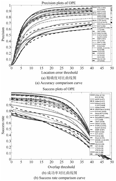
    图  9  50种目标跟踪算法在数据集OTB-2013上的总体性能对比, 这里只显示了排名前30的算法

    Fig.  9  The overall performance comparison of 50 object tracking algorithms in the data set OTB-2013, only the top 30 algorithms are shown here

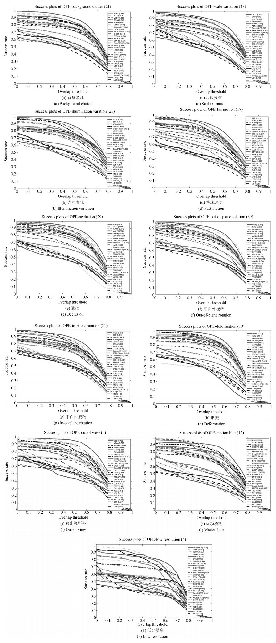
    图  10  50种目标跟踪算法, 在数据集OTB-2013中11种属性下的成功率曲线

    Fig.  10  50 object tracking algorithms, success rate curves under 11 attributes in data set OTB-2013

    表  1  各种目标跟踪算法的速度比较

    Table  1  Speed comparison of various object tracking algorithms

    基于相关滤波 AUC FPS 基于深度学习 AUC FPS
    MCPF[83] 0.677 0.5 VITAL[78] 0.710 1.5
    BACF[15] 0.645 35 ECO[19] 0.709 6
    LMCF[64] 0.628 85 SANet[81] 0.677 1
    LCT[65] 0.628 27 MDNet[80] 0.670 1
    SAMF[16] 0.597 7 C-COT[72] 0.659 0.3
    DSST[50] 0.554 24 ADNet[84] 0.659 3
    KCF[14] 0.551 172 HDT[85] 0.654 10
    CSK[13] 0.398 368 SRDCFdecon[63] 0.653 1
    MOSSE[12] 0.357 669 CF2[66] 0.562 11
    ECO-HC[19] 0.652 20 DeepLMCF[64] 0.646 8
    DeepSRDCF[62] 0.641 0.3
    SiamFC[73] 0.612 58
    DRT[63] 0.581 0.4
    下载: 导出CSV
  • [1] Yang H X, Shao L, Zheng F, Wang L, Song Z. Recent advances and trends in visual tracking:a review. Neurocomputing, 2011, 74(18):3823-3831 doi: 10.1016/j.neucom.2011.07.024
    [2] Smeulders A W M, Chu D M, Cucchiara R, Calderara S, Dehghan A, Shah M. Visual tracking:an experimental survey. IEEE Transactions on Pattern Analysis and Machine Intelligence, 2014, 36(7):1442-1468 doi: 10.1109/TPAMI.2013.230
    [3] Choi J Y, Sung K S, Yang Y K. Multiple vehicles detection and tracking based on scale-invariant feature transform. In: Proceedings of the 2007 IEEE Intelligent Transportation Systems Conference. Seattle, WA, USA: IEEE, 2007. 528-533
    [4] Bay H, Tuytelaars T, Van Gool L. SURF: speeded up robust features. In: Proceeding of Computer Vision-ECCV 2006. Lecture Notes in Computer Science, vol. 3951. Berlin, Heidelberg: Germany Springer, 2006. 404-417
    [5] Nguyen M H, Wünsche B, Delmas P, Lutteroth C. Modelling of 3D objects using unconstrained and uncalibrated images taken with a handheld camera. In: Proceedings of the Computer Vision, Imaging and Computer Graphics. Communications in Computer and Information Science, vol.274. Berlin, Heidelberg: Springer, 2011. 86-101
    [6] Kass M, Witkin A, Terzopoulos D. Snakes:active contour models. International Journal of Computer Vision, 1988, 1(4):321-331 doi: 10.1007/BF00133570
    [7] Welch G, Bishop G. An Introduction to the Kalman Filter. Chapel Hill, NC, USA: University of North Carolina at Chapel Hill, 2001.
    [8] Nummiaro K, Koller-Meier E, Van Gool L. An adaptive color-based particle filter. Image and Vision Computing, 2003, 21(1):99-110 doi: 10.1016/S0262-8856(02)00129-4
    [9] Du K, Ju Y F, Jin Y L, Li G, Li Y Y, Qian S L. Object tracking based on improved MeanShift and SIFT. In: Proceedings of the 2nd International Conference on Consumer Electronics, Communications and Networks. Yichang, China: IEEE, 2012. 2716-2719
    [10] 李冠彬, 吴贺丰.基于颜色纹理直方图的带权分块均值漂移目标跟踪算法.计算机辅助设计与图形学学报, 2011, 23(12):2059-2066 http://d.old.wanfangdata.com.cn/Periodical/jsjfzsjytxxxb201112017

    Li Guan-Bin, Wu He-Feng. Weighted fragments-based meanshift tracking using color-texture histogram. Journal of Computer-Aided Design and Computer Graphics, 2011, 23(12):2059-2066 http://d.old.wanfangdata.com.cn/Periodical/jsjfzsjytxxxb201112017
    [11] Exner D, Bruns E, Kurz D, Grundhöfer A, Bimber O. Fast and robust CAMShift tracking. In: Proceedings of the 2010 IEEE Computer Society Conference on Computer Vision and Pattern Recognition. San Francisco, CA, USA: IEEE, 2010. 9-16
    [12] Bolme D S, Beveridge J R, Draper B A, Lui Y M. Visual object tracking using adaptive correlation filters. In: Proceedings of the 2010 IEEE Computer Society Conference on Computer Vision and Pattern Recognition. San Francisco, CA, USA: IEEE, 2010. 2544-2550
    [13] Henriques J F, Caseiro R, Martins P, Batista J. Exploiting the circulant structure of tracking-by-detection with kernels. In: Proceedings of Computer Vision. Lecture Notes in Computer Science, vol.7575. Berlin, Heidelberg: Springer, 2012. 702-715
    [14] Henriques J F, Caseiro R, Martins P, Batista J. High-speed tracking with kernelized correlation filters. IEEE Transactions on Pattern Analysis and Machine Intelligence, 2015, 37(3):583-596 doi: 10.1109/TPAMI.2014.2345390
    [15] Galoogahi H K, Fagg A, Lucey S. Learning background-aware correlation filters for visual tracking. In: Proceedings of the 2017 IEEE International Conference on Computer Vision. Venice, Italy: IEEE, 2017. 1144-1152
    [16] Li Y, Zhu J. A scale adaptive kernel correlation filter tracker with feature integration. In: Proceedings of Computer Vision, Lecture Notes in Computer Science, vol.8926. Zurich, Switzerland: Springer, 2014. 254-265
    [17] Wu Y, Lim J, Yang M H. Online object tracking: a benchmark. In: Proceedings of the 2013 IEEE Conference on Computer Vision and Pattern Recognition. Portland, USA: IEEE, 2013. 2411-2418
    [18] Kristan M, Matas J, Leonardis A, Felsberg M, Cehovin L, Fernandez G, et al. The visual object tracking VOT2015 challenge results. In: Proceedings of the 2015 IEEE International Conference on Computer Vision Workshop. Santiago, USA: IEEE, 2015. 564-586
    [19] Yun S, Choi J, Yoo Y, Yun K M, Choi J Y. Action-decision networks for visual tracking with deep reinforcement learning. In: Proceedings of the 2017 IEEE Conference on Computer Vision and Pattern Recognition. Honolulu, HI, USA: IEEE, 2017. 1349-1358
    [20] Kristan M, Leonardis A, Matas J, Felsberg M, Pflugfelder R, Zajc L C, et al. The visual object tracking VOT2017 challenge results. In: Proceedings of the 2017 IEEE International Conference on Computer Vision Workshop. Venice, Italy: IEEE, 2017. 1949-1972
    [21] Zhang S P, Yao H X, Sun X, Lu X S. Sparse coding based visual tracking:review and experimental comparison. Pattern Recognition, 2013, 46(7):1772-1788 doi: 10.1016/j.patcog.2012.10.006
    [22] Gong H F, Sim J, Likhachev M, Shi J B. Multi-hypothesis motion planning for visual object tracking. In: Proceedings of the 2011 International Conference on Computer Vision. Barcelona, Spain: IEEE, 2011. 619-626
    [23] Sun D Q, Roth S, Black M J. Secrets of optical flow estimation and their principles. In: Proceedings of the 2010 IEEE Computer Society Conference on Computer Vision and Pattern Recognition. San Francisco, CA: IEEE, 2010. 2432-2439
    [24] Xu L, Jia J Y, Matsushita Y. Motion detail preserving optical flow estimation. In: Proceedings of the 2010 IEEE Computer Society Conference on Computer Vision and Pattern Recognition. San Francisco, CA, USA: IEEE, 2010. 1293-1300
    [25] Choi J, Kwon J, Lee K M. Visual tracking by reinforced decision making. Advances in Visual Computing, 2014. 270-280
    [26] Babenko B, Yang M H, Belongie S. Robust object tracking with online multiple instance learning. IEEE Transactions on Pattern Analysis and Machine Intelligence, 2011, 33(8):1619-1632 doi: 10.1109/TPAMI.2010.226
    [27] Kalal Z, Mikolajczyk K, Matas J. Tracking-learning-detection. IEEE Transactions on Pattern Analysis and Machine Intelligence, 2012, 34(7):1409-1422 doi: 10.1109/TPAMI.2011.239
    [28] Avidan S. Support vector tracking. IEEE Transactions on Pattern Analysis and Machine Intelligence, 2004, 26(8):1064-1072 doi: 10.1109/TPAMI.2004.53
    [29] Hare S, Saffari A, Torr P H S. Struck: structured output tracking with kernels. In: Proceedings of the 2011 IEEE International Conference on Computer Vision. Barcelona, Spain: IEEE, 2011. 263-270
    [30] Saffari A, Leistner C, Santner J, Godec M, Bischof H. On-line random forests. In: Proceedings of the IEEE 12th International Conference on Computer Vision Workshops. Kyoto, Japan: IEEE, 2009. 1393-1400
    [31] Babenko B, Yang M H, Belongie S. Visual tracking with online multiple instance learning. In: Proceedings of the 2009 IEEE Conference on Computer Vision and Pattern Recognition. Miami, FL: IEEE, 2009. 983-990
    [32] Jiang N, Liu W Y, Wu Y. Learning adaptive metric for robust visual tracking. IEEE Transactions on Image Processing, 2011, 20(8):2288-2300 doi: 10.1109/TIP.2011.2114895
    [33] Liu M, Wu C D, Zhang Y Z. Motion vehicle tracking based on multi-resolution optical flow and multi-scale Harris corner detection. In: Proceedings of the 2007 IEEE International Conference on Robotics and Biomimetics. Sanya, China: IEEE, 2007. 2032-2036
    [34] 吴垠, 李良福, 肖樟树, 刘侍刚.基于尺度不变特征的光流法目标跟踪技术研究.计算机工程与应用, 2013, 49(15):157-161 doi: 10.3778/j.issn.1002-8331.1211-0207

    Wu Yin, Li Liang-Fu, Xiao Zhang-Shu, Liu Shi-Gang. Optical flow motion tracking algorithm based on SIFT feature. Computer Engineering and Applications, 2013, 49(15):157-161 doi: 10.3778/j.issn.1002-8331.1211-0207
    [35] Rodríguez-Canosa G R, Thomas S, del Cerro J, Barrientos A, MacDonald B. A real-time method to detect and track moving objects (DATMO) from unmanned aerial vehicles (UAVs) using a single camera. Remote Sensing, 2012, 4(4):1090-1111 doi: 10.3390/rs4041090
    [36] 刘大千, 刘万军, 费博雯, 曲海成.前景约束下的抗干扰匹配目标跟踪方法.自动化学报, 2018, 44(6):1138-1152 http://www.aas.net.cn/CN/abstract/abstract19303.shtml

    Liu Da-Qian, Liu Wan-Jun, Fei Bo-Wen, Qu Hai-Cheng. A new method of anti-interference matching under foreground constraint for target tracking. Acta Automatica Sinica, 2018, 44(6):1138-1152 http://www.aas.net.cn/CN/abstract/abstract19303.shtml
    [37] 杨旭升, 张文安, 俞立.适用于事件触发的分布式随机目标跟踪方法.自动化学报, 2017, 43(8):1393-1401 http://www.aas.net.cn/CN/abstract/abstract19113.shtml

    Yang Xu-Sheng, Zhang Wen-An, Yu Li. Distributed tracking method for maneuvering targets with event-triggered mechanism. Acta Automatica Sinica, 2017, 43(8):1393-1401 http://www.aas.net.cn/CN/abstract/abstract19113.shtml
    [38] Kwolek B. CamShift-based tracking in joint color-spatial spaces. In: Proceedings of the Computer Analysis of Images and Patterns. Lecture Notes in Computer Science, vol.3691. Berlin, Heidelberg Germany: Springer, 2005. 693-700
    [39] Guo W H, Feng Z R, Ren X D. Object tracking using local multiple features and a posterior probability measure. Sensors, 2017, 17(4):739 doi: 10.3390/s17040739
    [40] Fu C H, Duan R, Kircali D, Kayacan E. Onboard robust visual tracking for UAVs using a reliable global-local object model. Sensors, 2016, 16(9):1406 doi: 10.3390/s16091406
    [41] Yuan G W, Zhang J X, Han Y H, Zhou H, Xu D. A multiple objects tracking method based on a combination of Camshift and object trajectory tracking. In: Proceedings of Advances in Swarm and Computational Intelligence. Lecture Notes in Computer Science, vol.9142. Beijing, China: Springer, 2015. 155-163
    [42] Huang S L, Hong J X. Moving object tracking system based on Camshift and Kalman filter. In: Proceedings of the 2011 IEEE International Conference on Consumer Electronics, Communications and Networks. Xianning, China: IEEE, 2011. 1423-1426
    [43] Ditlevsen S, Samson A. Estimation in the partially observed stochastic Morris-Lecar neuronal model with particle filter and stochastic approximation methods. Annals of Applied Statistics, 2014, 8(2):674-702 doi: 10.1214/14-AOAS729
    [44] Wang Z W, Yang X K, Xu Y, Yu S Y. CamShift guided particle filter for visual tracking. Pattern Recognition Letters, 2009, 30(4):407-413 doi: 10.1016/j.patrec.2008.10.017
    [45] 王鑫, 唐振民.一种改进的基于Camshift的粒子滤波实时目标跟踪算法.中国图象图形学报, 2010, 15(10):1507-1514 http://d.old.wanfangdata.com.cn/Periodical/zgtxtxxb-a201010013

    Wang Xin, Tang Zhen-Min. An improved camshift-based particle filter algorithm for real-time target tracking. Journal of Image and Graphics, 2010, 15(10):1507-1514 http://d.old.wanfangdata.com.cn/Periodical/zgtxtxxb-a201010013
    [46] Wang L, Chen F L, Yin H M. Detecting and tracking vehicles in traffic by unmanned aerial vehicles. Automation in Construction, 2016, 72:294-308 doi: 10.1016/j.autcon.2016.05.008
    [47] 张宏志, 张金换, 岳卉, 黄世霖.基于CamShift的目标跟踪算法.计算机工程与设计, 2006, 27(11):2012-2014 doi: 10.3969/j.issn.1000-7024.2006.11.032

    Zhang Hong-Zhi, Zhang Jin-Huan, Yue Hui, Huang Shi-Lin. Object tracking algorithm based on CamShift. Computer Engineering and Design, 2006, 27(11):2012-2014 doi: 10.3969/j.issn.1000-7024.2006.11.032
    [48] Danelljan M, Khan F S, Felsberg M, van de Weijer J. Adaptive color attributes for real-time visual tracking. In: Proceedings of the 2014 IEEE Conference on Computer Vision and Pattern Recognition. Columbus, OH, USA: IEEE, 2014. 1090-1097
    [49] Liu T, Wang G, Yang Q X. Real-time part-based visual tracking via adaptive correlation filters. In: Proceedings of the 2015 IEEE Conference on Computer Vision and Pattern Recognition. Boston, USA: IEEE, 2015. 4902-4912
    [50] Danelljan M, Häger G, Khan F S, Felsberg M. Accurate scale estimation for robust visual tracking. In: Proceedings British Machine Vision Conference. London, England: BMVA Press, 2014. 65.1-65.11
    [51] Zhu G B, Wang J Q, Wu Y, Zhang X Y, Lu H Q. MC-HOG correlation tracking with saliency proposal. In: Proceedings of the 13th AAAI Conference on Artificial Intelligence. Phoenix, USA: AAAI Press, 2016. 3690-3696
    [52] Bibi A, Mueller M, Ghanem B. Target Response Adaptation for Correlation Filter Tracking. In: Proceedings of the 2016 IEEE European Conference on Computer Vision Workshop. Amsterdam, Netherlands: IEEE, 2016. 419-433
    [53] O'Rourke S M, Herskowitz I, O'Shea E K. Yeast go the whole HOG for the hyperosmotic response. Trends in Genetics, 2002, 18(8):405-412 doi: 10.1016/S0168-9525(02)02723-3
    [54] Bertinetto L, Valmadre J, Golodetz S, Miksik O, Torr P H S. Staple: complementary learners for real-time tracking. In: Proceedings of the 2016 IEEE Conference on Computer Vision and Pattern Recognition. Las Vegas, USA: IEEE, 2016. 1401-1409
    [55] Kristan M, Pflugfelder R, Leonardis A, Matas J, Čehovin L, Nebehay G, et al. The visual object tracking VOT2014 challenge results. In: Proceedings of Computer Vision. Lecture Notes in Computer Science, vol.8926. Zurich, Switzerland: Springer, 2015. 191-217
    [56] Xu Y L, Wang J B, Li H, Li Y, Miao Z, Zhang Y F. Patch-based scale calculation for real-time visual tracking. IEEE Signal Processing Letters, 2016, 23(1):40-44 doi: 10.1109/LSP.2015.2479360
    [57] Akin O, Erdem E, Erdem A, Mikolajczyk K. Deformable part-based tracking by coupled global and local correlation filters. Journal of Visual Communication and Image Representation, 2016, 38:763-774 doi: 10.1016/j.jvcir.2016.04.018
    [58] Guo L S, Li J S, Zhu Y H, Tang Z Q. A novel features from accelerated segment test algorithm based on LBP on image matching. In: Proceedings of the 3rd IEEE International Conference on Communication Software and Networks. Xi'an, China: IEEE, 2011. 355-358
    [59] Calonder M, Lepetit V, Strecha C, Fua P. BRIEF: binary robust independent elementary features. In: Proceedings of Computer Vision. Lecture Notes in Computer Science, vol.6314. Heraklion, Crete: Springer, 2010. 778-792
    [60] Montero A S, Lang J, Laganiére R. Scalable kernel correlation filter with sparse feature integration. In: Proceedings of the 2015 IEEE International Conference on Computer Vision Workshop. Santiago, Chile: IEEE, 2015. 587-594
    [61] 张微, 康宝生.相关滤波目标跟踪进展综述.中国图象图形学报, 2017, 22(8):1017-1033 http://d.old.wanfangdata.com.cn/Periodical/zgtxtxxb-a201708001

    Zhang Wei, Kang Bao-Sheng. Recent advances in correlation filter-based object tracking:a review. Journal of Image and Graphics, 2017, 22(8):1017-1033 http://d.old.wanfangdata.com.cn/Periodical/zgtxtxxb-a201708001
    [62] Danelljan M, Häger G, Khan F S, Felsberg M. Learning spatially regularized correlation filters for visual tracking. In: Proceedings of the 2015 IEEE International Conference on Computer Vision. Santiago, Chile: IEEE, 2015. 4310-4318
    [63] Danelljan M, Häger G, Khan F S, Felsberg M. Adaptive decontamination of the training set: a unified formulation for discriminative visual tracking. In: Proceedings of the 2016 IEEE Conference on Computer Vision and Pattern Recognition. Las Vegas, USA: IEEE, 2016. 1430-1438
    [64] Wang M M, Liu Y, Huang Z Y. Large margin object tracking with circulant feature maps. In: Proceedings of the 2017 IEEE Conference on Computer Vision and Pattern Recognition. Honolulu, HI, USA: IEEE, 2017. 4800-4808
    [65] Ma C, Yang X K, Zhang C Y, Yang M H. Long-term correlation tracking. In: Proceedings of the 2015 IEEE Conference on Computer Vision and Pattern Recognition. Boston, USA: IEEE, 2015. 5388-5396
    [66] Ma C, Huang J B, Yang X K, Yang M H. Hierarchical convolutional features for visual tracking. In: Proceedings of the 2015 IEEE International Conference on Computer Vision. Santiago, Chile: IEEE, 2015. 3074-3082
    [67] Wang N Y, Yeung D Y. Ensemble-based tracking: aggregating crowdsourced structured time series data. In: Proceedings of the 31st International Conference on Machine Learning. Beijing, China, 2014. 1107-1115
    [68] Wang N Y, Yeung D Y. Learning a deep compact image representation for visual tracking. In: Proceedings of the 26th International Conference on Neural Information Processing Systems. Lake Tahoe, Nevada: Curran Associates Inc., 2013. 809-817
    [69] Wang D, Lu H C, Yang M H. Least soft-threshold squares tracking. In: Proceedings of the 2013 IEEE Conference on Computer Vision and Pattern Recognition. Portland, OR, USA: IEEE, 2013. 2371-2378
    [70] Hare S, Golodetz S, Saffari A, Vineet V, Cheng M M, Hicks S L, et al. Struck:structured output tracking with kernels. IEEE Transactions on Pattern Analysis and Machine Intelligence, 2016, 38(10):2096-2109 doi: 10.1109/TPAMI.2015.2509974
    [71] 管皓, 薛向阳, 安志勇.深度学习在视频目标跟踪中的应用进展与展望.自动化学报, 2016, 42(6):834-847 http://www.aas.net.cn/CN/abstract/abstract18874.shtml

    Guan Hao, Xue Xiang-Yang, An Zhi-Yong. Advances on application of deep learning for video object tracking. Acta Automatica Sinica, 2016, 42(6):834-847 http://www.aas.net.cn/CN/abstract/abstract18874.shtml
    [72] Danelljan M, Robinson A, Khan F S, Felsberg M. Beyond correlation filters: Learning continuous convolution operators for visual tracking. In: Proceedings of Computer Vision. Lecture Notes in Computer Science, vol.9909. Amsterdam, Netherlands: Springer, 2016. 472-488
    [73] Bertinetto L, Valmadre J, Henriques J F, Vedaldi A, Torr P H S. Fully-convolutional siamese networks for object tracking. In: Proceedings of Computer Vision. Lecture Notes in Computer Science, vol.9914. Amsterdam, Netherlands: Springer, 2016. 850-865
    [74] Ding J W, Huang Y Z, Liu W, Huang K Q. Severely blurred object tracking by learning deep image representations. IEEE Transactions on Circuits and Systems for Video Technology, 2016, 26(2):319-331 doi: 10.1109/TCSVT.2015.2406231
    [75] Dai L, Zhu Y S, Luo G B, He C. A low-complexity visual tracking approach with single hidden layer neural networks. In: Proceedings of the 13th International Conference on Control Automation Robotics and Vision. Singapore: IEEE, 2014. 810-814
    [76] Li P X, Wang D, Wang L J, Lu H C. Deep visual tracking:review and experimental comparison. Pattern Recognition, 2018, 76:323-338 doi: 10.1016/j.patcog.2017.11.007
    [77] Nam H, Baek M, Han B. Modeling and propagating CNNs in a tree structure for visual tracking. In: Proceedings of the 2016 IEEE Conference on Computer Vision and Pattern Recognition. Las Vegas, USA: IEEE, 2016. 2137-2155
    [78] Song Y B, Ma C, Wu X H, Gong L J, Bao L C, Zuo W M, et al. Visual tracking via adversarial learning. In: Proceedings of the 2018 IEEE Conference on Computer Vision and Pattern Recognition. Salt Lake City, Utah, USA: IEEE, 2018. 1084-1093
    [79] Wu Y, Lim J, Yang M H. Object tracking benchmark. IEEE Transactions on Pattern Analysis and Machine Intelligence, 2015, 37(9):1834-1848 doi: 10.1109/TPAMI.2014.2388226
    [80] Nam H, Han B. Learning multi-domain convolutional neural networks for visual tracking. In: Proceedings of the 2016 IEEE Conference on Computer Vision and Pattern Recognition. Las Vegas, USA: IEEE, 2016. 4293-4302
    [81] Fan H, Ling H B. SANet: structure-aware network for visual tracking. In: Proceedings of the 2017 IEEE Conference on Computer Vision and Pattern Recognition Workshops. Honolulu, HI, USA: IEEE, 2017. 2217-2224
    [82] Han B, Sim J, Adam H. BranchOut: regularization for online ensemble tracking with convolutional neural networks. In: Proceedings of the 2017 IEEE Conference on Computer Vision and Pattern Recognition. Honolulu, HI, USA: IEEE, 2017. 521-530
    [83] Zhang T Z, Xu C S, Yang M H. Multi-task correlation particle filter for robust object tracking. In: Proceedings of the 2017 IEEE Conference on Computer Vision and Pattern Recognition. Honolulu, HI, USA: IEEE, 2017. 4819-4827
    [84] Yun S, Choi J, Yoo Y, Yun K M, Choi J Y. Action-decision networks for visual tracking with deep reinforcement learning. In: Proceedings of the 2017 IEEE Conference on Computer Vision and Pattern Recognition. Honolulu, HI, USA: IEEE, 2017. 1349-1358
    [85] Qi Y K, Zhang S P, Qin L, Yao H X, Huang Q M, Lim J, et al. Hedged deep tracking. In: Proceedings of the 2016 IEEE Conference on Computer Vision and Pattern Recognition. Las Vegas, USA: IEEE, 2016. 4303-4311
    [86] Gao J Y, Zhang T Z, Yang X S, Xu C S. Deep relative tracking. IEEE Transactions on Image Processing, 2017, 26(4):1845-1858 doi: 10.1109/TIP.2017.2656628
  • 期刊类型引用(8)

    1. 赵利军,白硕,李欣刚,赵娜. 改进BIM模型的高层办公建筑节能优化仿真. 计算机仿真. 2024(08): 281-285 . 百度学术
    2. 季伟东,岳玉麒,王旭,林平. 基于降维和聚类的大规模多目标自然计算方法. 系统仿真学报. 2023(01): 41-56 . 百度学术
    3. 文家燕,闻海潮,程洋,罗绍猛,何伟朝. 基于GWO-NSGA-Ⅱ混合算法的露天矿低碳运输调度. 工矿自动化. 2023(02): 94-101 . 百度学术
    4. 尹传忠,彭海红,陶学宗,张子昂. 基于改进NSGA-Ⅱ的多式联运协同优化. 上海海事大学学报. 2023(04): 39-44+116 . 百度学术
    5. 黄朝志,耿永民,原红卫. 基于NSGA-Ⅱ的局部范围搜索算法的电机参数优化. 电机与控制应用. 2022(06): 9-18 . 百度学术
    6. 杨生仁,孙超,杜太升. 基于静态模糊聚类算法求解最短路径问题. 中国储运. 2022(10): 163-164 . 百度学术
    7. 张伟,黄卫民. 基于种群分区的多策略自适应多目标粒子群算法. 自动化学报. 2022(10): 2585-2599 . 本站查看
    8. 韩飞,张葛祥. 基于超混沌系统的网络用户隐私信息加密仿真. 计算机仿真. 2021(12): 295-298+405 . 百度学术

    其他类型引用(14)

  • 加载中
  • 图(10) / 表(1)
    计量
    • 文章访问数:  10106
    • HTML全文浏览量:  3769
    • PDF下载量:  3894
    • 被引次数: 22
    出版历程
    • 收稿日期:  2018-05-04
    • 录用日期:  2018-07-16
    • 刊出日期:  2019-07-20

    目录

    /

    返回文章
    返回