

Intelligent Selection of Simulation Experiment Design Methods Based on Hybrid Reasoning
-
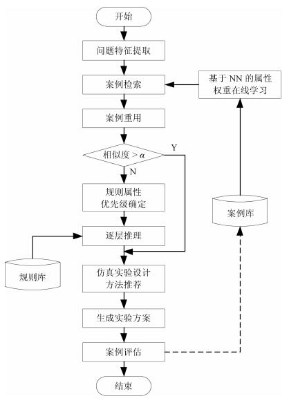
摘要: 针对仿真实验设计方法众多而在实际应用中难以准确选择的问题,提出一种用于仿真实验设计方法智能选择的混合推理方法.首先,给出了基于混合推理的仿真实验智能化设计流程;然后,针对案例检索策略,将仿真实验设计案例的属性分为三种类型,分别给出其属性差异度量模型及特征值归一化方法,并采用训练后的神经网络模型分配属性权重;进一步,当推荐的案例未能满足给定的相似度阈值时,引入属性优先级的概念,提出了一种基于规则的柔性逐层推理方法;在此基础上,设计了案例库和规则库;最后,通过实验验证了所提出方法的有效性.Abstract: Due to the variety of simulation experiment design methods, it is difficult to choose an appropriate method in the practical application. In order to solve this problem, a hybrid reasoning method for selecting simulation experiment design methods intelligently is proposed in this paper. Firstly, a workflow of intelligent design of simulation experiment based on hybrid reasoning is given. Then, the attributes of cases are divided into three types towards the case retrieval strategy. The difference measurement models and methods are given for each type. Meanwhile, the weight assignment method of attributes based on neural network is given. Furthermore, when the recommended case fails to meet the given similarity threshold, a rule-based flexible layer-by-layer reasoning (RBFLR) method is proposed by introducing the concept of attribute priority. Based on above, the case base and the rule base are designed. Finally, the effectiveness of the proposed method is verified by experiments.1) 本文责任编委 刘艳军
-
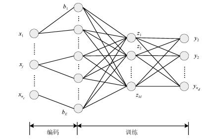
图 3 基于NN的属性权重分配网络结构
Fig. 3 Network structure of attribute weight assignment based on neural network
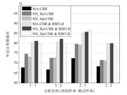
图 5 不同分配比例下各推理方法的平均分配准确率
Fig. 5 Averaging classification accuracy of different assignment proportions
表 1 案例属性
Table 1 Attributes of the cases
ID 属性 属性取值 属性类型 1 实验目的 $\text{EP}\in\textbf{ N}$ 语义型离散 2 实验点分布 $\text{ED}\in\textbf{ N}$ 语义型离散 3 系统复杂度假设 $\text{SC}\in\textbf{ N}$ 语义型离散 4 二因子交互效应估计 $\text{FI}\in\textbf{ N}$ 语义型离散 5 模型独立性 $\text{MI}\in\textbf{ N}$ 语义型离散 6 处理群组因子 $\text{CG}\in\textbf{ N}$ 语义型离散 7 实验点可扩展性 $\text{EE}\in\textbf{ N}$ 语义型离散 8 水平数 $\text{FL}\in\textbf{ N}$ 语义型离散 9 实验次数 $\text{EN}\in\textbf{ N}$ $^{+}$ 实数型离散 10 因子数 $\text{FN}\in\textbf{ N}$ $^{+}$ 实数型离散 11 仿真实验设计方法 $\text{EM}\in\textbf{ N}$ $^{+}$ 语义型离散  下载: 导出CSV
表 2 规则属性
Table 2 Attributes of the rules
ID 属性 属性取值 属性类型 优先级 1 实验目的 $\text{EP}\in\textbf{ N}$ 语义型离散 ${{k}_{1}}$ 2 实验点分布 $\text{ED}\in\textbf{ N}$ 语义型离散 ${{k}_{2}}$ 3 系统复杂度假设 $\text{SC}\in\textbf{ N}$ 语义型离散 ${{k}_{3}}$ 4 二因子交互效应估计 $\text{FI}\in\textbf{ N}$ 语义型离散 ${{k}_{4}}$ 5 模型独立性 $\text{MI}\in\textbf{ N}$ 语义型离散 ${{k}_{5}}$ 6 处理群组因子 $\text{CG}\in\textbf{ N}$ 语义型离散 ${{k}_{6}}$ 7 实验点可扩展性 $\text{EE}\in\textbf{ N}$ 语义型离散 ${{k}_{7}}$ 8 水平数 $\text{FL}\in\textbf{ N}$ 语义型离散 ${{k}_{8}}$ 9 实验次数 $\text{EN}\in [{s}_{1}, {s}_{2}]$ 实数型区间 ${{k}_{9}}$ 10 因子数 $\text{FN}\in [{n}_{1}, {n}_{2}]$ 实数型区间 ${{k}_{10}}$ 11 仿真实验设计方法 $\text{EM}\in\textbf{ N}$ $^{+}$ 语义型离散 $/$ 备注: EP $\in $ {1)寻找重要因子, 2)寻找稳健参数, 3)优化, 4)不确定性分析, 5)灵敏度分析, 6)方差分析, 7)综合评估}; ED $\in $ {1)均匀性, 2)正交性, 3)空间填充性, 4)随机性, 5)鲁棒性, 6)序贯性}; SC $\in $ {1)一阶多项式(主效应模型), 2)一阶多项式+二因子交互效应, 3)二阶多项式(含完全平方项), 4)高阶交互效应}; FI $\in $ {1)能, 2)否}; MI $\in $ {1)是, 2)否}; CG $\in $ {1)能, 2)否}; EE $\in $ {1)能, 2)否}; FL $\in $ {1) 2$ \sim $3水平为主, 2) 4$ \sim $10水平为主, 3)大于10水平为主, 4)水平较为分散}; EN $\in $ {1) $[1, n)$, 2) $[n, +\infty)$, 3) $[{{2}^{n}}, +\infty)$}, 其中$n$为因子数; FN $\in $ {1) $[2, 13]$, 2) $[14, 50]$, 3) $[51, 100]$, 4) $[101, 500]$, 5) $[501, +\infty)$}; EM $\in $ {1)全面析因设计, 2)分式析因设计, 3)正交设计, 4)均匀设计, 5)拉丁超立方抽样, 6)蒙特卡罗抽样, 7)拟蒙特卡罗抽样, 8)重要性抽样, 9)中心复合设计, 10)稳健设计, 11)顺序分支法, 12)迭代分式析因设计, 13)二阶段组筛选法, 14) Trocine筛选流程}.
下载: 导出CSV
表 3 规则库
Table 3 Rule base
ID $Pc$ $Cq$ 1 $\text{EP}=2$ $\text{EM}=\left\{ 10 \right\}$ 2 $\text{ED}=3$ $\text{EM}=\left\{ 3, 4, 5 \right\}$ 3 $\text{CG}=1$ $\text{EM}=\left\{ 11, 12, 13, 14 \right\}$ $\vdots $ $\vdots $ $\vdots $ 60 $\text{FL}=4$, $\text{EN}=2$, $\text{FN}=3$ $\text{EM}=\left\{ 11, 14 \right\}$
下载: 导出CSV
表 4 规则的条件属性优先级
Table 4 Priority of condition attribute for the rules
EP ED SC FI MI CG EE FL EN FN 5 2 3 3 4 4 3 1 1 1
下载: 导出CSV
表 5 案例库
Table 5 Case base
ID EP ED SC FI MI CG EE FL EN FN EM 1 6 2 2 1 1 2 2 1 32 5 1 2 5 3 1 1 1 2 2 1 8 7 3 3 5 3 2 1 1 2 1 3 500 7 5 $\vdots $ $\vdots $ $\vdots $ $\vdots $ $\vdots $ $\vdots $ $\vdots $ $\vdots $ $\vdots $ $\vdots $ $\vdots $ $\vdots $ 142 3 1 1 1 1 2 2 2 10 8 4
下载: 导出CSV
表 6 不同推理方法的平均分类准确率($\%$)
Table 6 Averaging classification accuracy of different reasoning methods ($\%$)
推理方法 分配比例 1 : 1 3 : 2 2 : 1 2 : 3 MA-CBR 67.61 66.67 72.34 68.24 NN$\_$Rel-CBR 74.51 72.46 79.57 71.41 NN$\_$Sal-CBR 73.10 72.63 79.15 71.18 MA-CBR&RBFLR 80.28 80.70 85.11 ${\bf 80.00}$ NN$\_$Rel-CBR & RBFLR ${\bf 81.13}$ ${\bf 82.11}$ 85.74 ${\bf 80.00}$ NN$\_$Sal-CBR & RBFLR 79.58 80.00 ${\bf 86.60}$ 78.59
下载: 导出CSV
-
[1] Kleijnen J P C[著], 张列刚, 张建康, 刘兴科[译].仿真实验设计与分析.北京: 电子工业出版社, 2010. 1-136Kleijnen J P C[Author], Zhang Lie-Gang, Zhang Jian-Kang, Liu Xing-Ke[Translator]. Design and Analysis of Simulation Experiments. Beijing: Publishing House of Electronics Industry, 2010. 1-136 [2] Wu Y L, Song X, Gong G H. Real-time load balancing scheduling algorithm for periodic simulation models. Simulation Modelling Practice and Theory, 2015, 52:123-134 doi: 10.1016/j.simpat.2015.01.001 [3] Simpson T W, Booker A J, Ghosh D, Giunta A A, Koch P N, Yang R J. Approximation methods in multidisciplinary analysis and optimization:a panel discussion. Structural and Multidisciplinary Optimization, 2004, 27(5):302-313 [4] Trocine L, Malone L C. Experimental design and analysis: an overview of newer, advanced screening methods for the initial phase in an experimental design. In: Proceedings of the 33rd Conference on Winter Simulation. Arlington, Virginia: IEEE, 2001. 169-178 [5] Wang G G, Shan S. Review of metamodeling techniques in support of engineering design optimization. Journal of Mechanical Design, 2007, 129(4):370-380 doi: 10.1115/1.2429697 [6] Sanchez S M, Wan H. Work smarter, not harder: a tutorial on designing and conducting simulation experiments. In: Proceedings of the 2012 Winter Simulation Conference. Berlin, Germany: IEEE, 2012. 1-15 [7] Burnaev E, Panin I, Sudret B. Efficient design of experiments for sensitivity analysis based on polynomial chaos expansions. Annals of Mathematics and Artificial Intelligence, 2017, 81(1-2):187-207 doi: 10.1007/s10472-017-9542-1 [8] Garud S S, Karimi I A, Kraft M. Design of computer experiments:a review. Computers & Chemical Engineering, 2017, 106:71-95 http://d.old.wanfangdata.com.cn/OAPaper/oai_doaj-articles_b0be64b1b06c0793fe44ccf7da68bb9b [9] Fang K T, Lin D K J, Winker P, Zhang Y. Uniform design:theory and application. Technometrics, 2000, 42(3):237-248 doi: 10.1080/00401706.2000.10486045 [10] Sheldon M R. Simulation (Fifth edition). San Diego:Academic Press, 2012. 153-232 [11] Husslage B G M, Rennen G, van Dam E R, den Hertog D. Space-filling Latin hypercube designs for computer experiments. Optimization and Engineering, 2011, 12(4):611-630 doi: 10.1007/s11081-010-9129-8 [12] Damblin G, Couplet M, Iooss B. Numerical studies of space-filling designs:optimization of Latin hypercube samples and subprojection properties. Journal of Simulation, 2013, 7(4):276-289 doi: 10.1057/jos.2013.16 [13] Tong C. Refinement strategies for stratified sampling methods. Reliability Engineering & System Safety, 2006, 91(10-11):1257-1265 http://www.wanfangdata.com.cn/details/detail.do?_type=perio&id=1df7de336bbf9bd363998586d5bd0ebf [14] Li W, Lu L Y, Xie X T, Yang M. A novel extension algorithm for optimized Latin hypercube sampling. Journal of Statistical Computation and Simulation, 2017, 87(13):2549-2559 doi: 10.1080/00949655.2017.1340475 [15] Williamson D. Exploratory ensemble designs for environmental models using k-extended Latin hypercubes. Environmetrics, 2015, 26(4):268-283 doi: 10.1002/env.2335 [16] Kleijnen J P C, Sanchez S M, Lucas T W, Cioppa T M. State-of-the-art review:a user's guide to the brave new world of designing simulation experiments. Informs Journal on Computing, 2005, 17(3):263-289 doi: 10.1287/ijoc.1050.0136 [17] Bursztyn D, Steinberg D M. Comparison of designs for computer experiments. Journal of Statistical Planning and Inference, 2006, 136(3):1103-1119 doi: 10.1016/j.jspi.2004.08.007 [18] 赵辉, 严爱军, 王普.提高案例推理分类器的可靠性研究.自动化学报, 2014, 40(9):2029-2036 http://www.aas.net.cn/CN/abstract/abstract18475.shtmlZhao Hui, Yan Ai-Jun, Wang Pu. On improving reliability of case-based reasoning classifier. Acta Automatica Sinica, 2014, 40(9):2029-2036 http://www.aas.net.cn/CN/abstract/abstract18475.shtml [19] 苏锑, 杨明, 王春香, 唐卫, 王冰.一种基于分类回归树的无人车汇流决策方法.自动化学报, 2018, 44(1):35-43 http://www.aas.net.cn/CN/abstract/abstract19202.shtmlSu Ti, Yang Ming, Wang Chun-Xiang, Tang Wei, Wang Bing. Classification and regression tree based traffic merging for method self-driving vehicles. Acta Automatica Sinica, 2018, 44(1):35-43 http://www.aas.net.cn/CN/abstract/abstract19202.shtml [20] 郑文博, 王坤峰, 王飞跃.基于贝叶斯生成对抗网络的背景消减算法.自动化学报, 2018, 44(5):878-890 http://www.aas.net.cn/CN/abstract/abstract19279.shtmlZheng Wen-Bo, Wang Kun-Feng, Wang Fei-Yue. Background subtraction algorithm with Bayesian generative adversarial networks. Acta Automatica Sinica, 2018, 44(5):878-890 http://www.aas.net.cn/CN/abstract/abstract19279.shtml [21] Richhariya B, Tanveer M. EEG signal classification using universum support vector machine. Expert Systems with Applications, 2018, 106:169-182 doi: 10.1016/j.eswa.2018.03.053 [22] Deng Y, Ren Z Q, Kong Y Y, Bao F, Dai Q H. A hierarchical fused fuzzy deep neural network for data classification. IEEE Transactions on Fuzzy Systems, 2017, 25(4):1006-1012 doi: 10.1109/TFUZZ.2016.2574915 [23] 万秋生.复杂仿真实验设计与监控技术研究[硕士学位论文], 哈尔滨工业大学, 中国, 2012. 25-30Wan Qiu-Sheng. The Technology of Designing and Monitoring for Complex Simulation Experiments[Master thesis], Harbin Institute of Technology, China, 2012. 25-30 [24] Li W, Lu L Y, Liu Z Z, Ma P, Yang M. HIT-SEDAES: an integrated software environment for simulation experiment design, analysis and evaluation. International Journal of Modeling, Simulation, and Scientific Computing, 2016, 7(3): Article No.1650027 [25] Im K H, Park S C. Case-based reasoning and neural network based expert system for personalization. Expert Systems with Applications, 2007, 32(1):77-85 http://www.wanfangdata.com.cn/details/detail.do?_type=perio&id=43719736fdd3ca8416f853887e59ec35 [26] Ahn H, Kim K J. Bankruptcy prediction modeling with hybrid case-based reasoning and genetic algorithms approach. Applied Soft Computing, 2009, 9(2):599-607 doi: 10.1016/j.asoc.2008.08.002 [27] Biswas S K, Chakraborty M, Singh H R, Devi D, Purkayastha B, Das A K. Hybrid case-based reasoning system by cost-sensitive neural network for classification. Soft Computing, 2017, 21(24):7579-7596 doi: 10.1007/s00500-016-2312-x -

 下载:
下载:

计量
- 文章访问数: 2484
- HTML全文浏览量: 503
- PDF下载量: 393
- 被引次数: 0
