

-
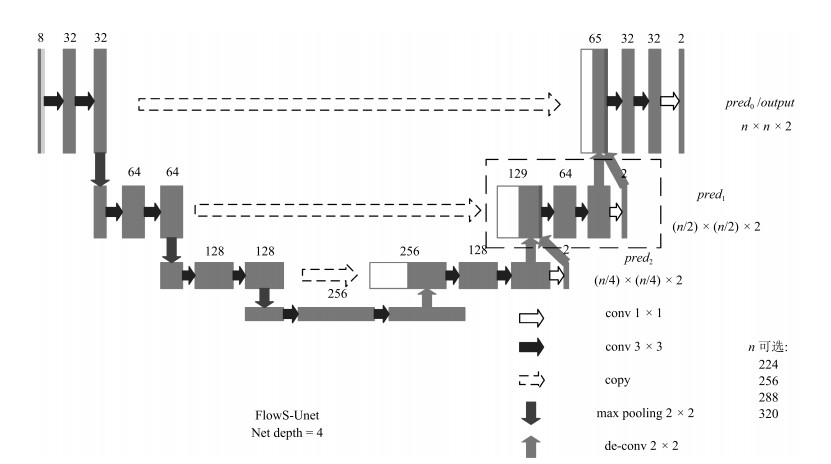
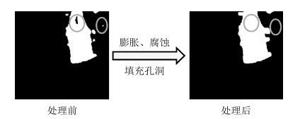
摘要: 针对目前人为探察土地资源利用情况的任务繁重、办事效率低下等问题, 提出了一种基于深度卷积神经网络的建筑物变化检测方法, 利用高分辨率遥感图像实时检测每个区域新建与扩建的建筑物, 以方便对土地资源进行有效管理.本文受超列(Hypercolumn)和FlowNet中的细化(Refinement)结构启发, 将细化和其他改进应用到U-Net, 提出FlowS-Unet网络.首先对遥感图像裁剪、去噪、标注语义制作数据集, 将该数据集划分为训练集和测试集, 对训练集进行数据增强, 并根据训练集图像的均值和方差对所有图像进行归一化; 然后将训练集输入集成了多尺度交叉训练、多重损失计算、Adam优化的全卷积神经网络FlowS-Unet中进行训练; 最后对网络模型的预测结果进行膨胀、腐蚀以及孔洞填充等后处理得到最终的分割结果.本文以人工分割结果为参考标准进行对比测试, 用FlowS-Unet检测得到的F1分数高达0.943, 明显优于FCN和U-Net的预测结果.实验结果表明, FlowS-Unet能够实时准确地将新建与扩建的建筑物变化检测出来, 并且该模型也可扩展到其他类似的图像检测问题中.
-
关键词:
- FlowS-Unet /
- 建筑物变化检测 /
- 全卷积神经网络 /
- 多尺度交叉训练 /
- 多重损失
Abstract: Since manually detecting the situation of land resource utilization is arduous and inefficient, a smart building change detection method based on deep convolutional network is proposed, which can detect newly emerged or expanded buildings in each region of the high-resolution remote sensing images at real-time, thus can be used to manage the land resources efficiently. This article proposes a model named FlowS-Unet by applying refinement and other improvements to U-Net, which was inspired by hypercolumns and the refinement structure in FlowNet. First, the remote sensing images were cropped, denoised, and semantically annotated to form the dataset which is further divided into the training set and testing set, the training set is augmented to get enough training samples, and the mean value and variance of all training images are calculated and used to normalize the dataset; Second, the training set is fed into the fully convolutional network FlowS-Unet for training, which integrates multi-scale cross training, multiple losses and Adam algorithm for its optimization. Finally, the predicted result of FlowS-Unet is further post-processed with dilating, eroding and hole-filling to get the final segmentation result. By using manually segmented results as the ground truth, a comparison with several different algorithms shows that the F1 score of FlowS-Unet is as high as 0.943, which is apparently better than the predicted results of fully convolutional networks (FCN) and U-Net. Experimental results indicate that the newly emerged or expanded buildings can be accurately detected at real time with FlowS-Unet. This model can also be applied to other similar image detection problems.-
Key words:
- FlowS-Unet /
- change detection for buildings /
- fully convolutional networks (FCN) /
- multi-scale cross training /
- multiple losses
-
在工业生产和社会生活中, 存在着大量的复杂系统, 如非线性耦合机械系统[1]、超临界机组[2]等. 这些复杂系统线性化时通常包含了不可控模态, 给其控制器设计与分析带来了挑战. 在过去十几年里, 这类称之为高阶非线性系统的自适应控制问题吸引了很多研究者的关注. Lin等在文献[3-4]中提出了一种新的构造性设计框架−增加幂次积分法, 有效解决了高阶非线性系统的镇定与实际跟踪问题. 借助于这一方法, 文献[5-19]研究了不同条件下高阶不确定非线性系统的自适应控制问题, 取得了一系列研究成果. 值得指出的是, 上述绝大多数研究结果都要求系统的幂次信息完全已知. 然而, 在一些实际应用中, 由于控制系统本身与周围环境存在着各种不确定因素, 使得系统的幂次信息可能无法精确获取. 因此, 进一步探讨具有未知幂次的高阶非线性系统的控制器设计是很有意义并值得研究的问题.
针对具有未知幂次的高阶非线性系统, 文献[20-21]采用改进的增加幂次积分法, 分别给出了状态反馈和输出反馈控制算法. 然而, 这些算法没有考虑系统函数的不确定性, 且需要假设系统的幂次上界信息已知. 文献[22]结合增加幂次积分技术和自适应控制方法, 解决了具有未知幂次和不确定参数的高阶非线性系统的自适应控制问题. 最近, 针对一类具有未知时变幂次的高阶非线性系统, 文献[23]利用障碍李雅普诺夫方法给出了满足全状态约束条件的自适应控制方案. 但文献[22-23]所提控制方案仍然要求系统幂次的上界已知. 为去除这一假设条件, 文献[24]采用增加幂次积分技术和逻辑切换方法, 设计了一种全局切换自适应镇定方案. 该方案的不足在于切换控制信号是非光滑的, 可能会引起抖振问题, 从而激发系统中的高频未建模动态. 为此, 文献[25]利用动态增益法, 提出了一种光滑自适应状态反馈控制器, 但这种控制器仅适用于相对阶为2的非线性系统.
基于以上讨论, 本文研究了一类具有未知幂次的高阶不确定非线性系统的自适应跟踪控制问题. 结合积分反推技术和障碍李雅普诺夫函数, 提出了一种新颖的自适应状态反馈控制策略. 本文所得到的控制策略具有如下优点: 1) 采用对数型障碍李雅普诺夫函数[26-27]解决了系统幂次未知与模型不确定带来的技术难题; 2) 所提出的自适应控制策略中没有包含虚拟控制律的导数信息, 避免了积分反推法中的“计算膨胀”问题; 3) 所设计控制器能够确保闭环系统的所有信号一致有界. 最后, 仿真结果验证了本文理论结果的有效性.
本文采用如下符号:
$ {\bf{R}} $ ,${\bf{R}}_{\geq{{0}}}$ ,${\bf{R}}_{ > {{0}}}$ 分别表示实数、非负实数和正实数集合.$ {{\bf{R}}}^n $ 表示$ n $ 维实向量集合.$ {\rm{sign}}(s) $ 表示变量$ s $ 的符号函数. 对任意正常数$ q $ , 定义$ [s]^q = {\rm{sign}}(s)|s|^q $ .${\bf{Q}}_{{\rm{odd}}}^{\ge 1}$ 表示分子和分母都是正奇整数的所有有理数的集合.1. 问题描述与预备知识
1.1 问题描述
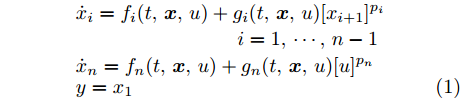
考虑如下高阶不确定非线性系统
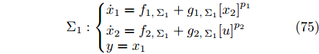
$$ \begin{split} & \dot{x}_i = f_i(t,{\boldsymbol{x}},u)+g_i(t,{\boldsymbol{x}},u)[x_{i+1}]^{p_i}\\ &\qquad\qquad\qquad\;\;\;\;\quad i = 1,\cdots,n-1\\ &\dot{x}_n = f_n(t,{\boldsymbol{x}},u)+g_n(t,{\boldsymbol{x}},u)[u]^{p_n}\\& y = x_1 \end{split} $$ (1) 其中,
${\boldsymbol{x}} = [x_1,\cdots,x_n]^{\rm{T}}\in {{\bf{R}}}^n$ 是系统的状态向量, 初始值${\boldsymbol{x}}(0) = [x_1(0),\cdots,x_n(0)]^{\rm{T}}$ ,$\bar{{\boldsymbol{x}}}_i = [x_1,\cdots,x_i]^{\rm{T}}\in {{\bf{R}}}^i$ ,$i = 1,\cdots,n$ ;$ u \in {{\bf{R}}} $ 和$ y \in {{\bf{R}}} $ 分别是控制输入和系统输出;$ p_i\in {\bf{Q}}_{{\rm{odd}}}^{\ge 1} $ ,$i = 1,\cdots,n$ 是系统(1)的未知幂次. 系统函数$ f_i, g_i:{{\bf{R}}}_{\ge0}\times {{\bf{R}}}^n\times {{\bf{R}}}\rightarrow {{\bf{R}}} $ ,$i = 1,\cdots,n$ 在$ t $ 上分段连续, 且关于$ {\boldsymbol{x}} $ 和$ u $ 满足局部Lipschitz条件. 本文的控制目标是设计自适应控制器$ u $ , 使得系统输出$ y $ 跟踪期望轨迹$ y_r $ , 同时确保闭环系统的所有信号皆有界.注 1. 不同于文献[20-25]中的研究结果, 本文中系统幂次无需满足
$ p_1\ge p_2\ge \cdots\ge p_n $ .假设 1. 存在未知的连续函数
$\bar{f}_{il}(\bar{{\boldsymbol{x}}}_i) : {{\bf{R}}}^{i}\rightarrow {{\bf{R}}}_{\geq0}$ ,$ \underline{g}_i(\bar{{\boldsymbol{x}}}_i): {{\bf{R}}}^{i}\rightarrow {{\bf{R}}}_{>0} $ 和$ \bar{g}_i(\bar{{\boldsymbol{x}}}_i): {{\bf{R}}}^{i}\rightarrow {{\bf{R}}}_{>0} $ , 满足$$ |f_i(t,{\boldsymbol{x}},u)|\le \sum\limits_{l = 1}^{j_i}|x_{i+1}|^{q_{il}}\bar{f}_{il}(\bar{{\boldsymbol{x}}}_i) $$ (2) $$ 0<\underline{g}_i(\bar{{\boldsymbol{x}}}_i)\le g_i(t,{\boldsymbol{x}},u)\le \bar{g}_i(\bar{{\boldsymbol{x}}}_i) $$ (3) 其中,
$i = 1,\cdots,n$ ,$l = 1,\cdots,j_i$ ,$ j_i $ 为有限正整数,$ q_{il} $ 为满足$ 0\le q_{i1}<q_{i2}<\cdots<q_{ij_i}<p_i $ 的正常数.注 2. 假设1表明了本文所提控制算法无需知晓系统函数
$ g_i(t,{\boldsymbol{x}},u) $ ,$ f_i(t,{\boldsymbol{x}},u) $ 及相应的界函数$ \underline{g}_i(\bar{{\boldsymbol{x}}}_{i}) $ ,$ \bar{g}_i(\bar{{\boldsymbol{x}}}_{i}) $ ,$ \bar{f}_{il}(\bar{{\boldsymbol{x}}}_i) $ 的解析表达式.假设 2. 期望轨迹
$ y_r $ 为连续可微函数, 且存在未知正常数$ B_r $ , 满足$$ |y_r(t)|+|\dot{y}_r(t)|\le B_r,t\ge 0 $$ (4) 1.2 预备知识
引理 1[28]. 考虑初值问题
$$ \dot{\boldsymbol{\eta}}_r(t) = h_r(t,{\boldsymbol{\eta}}_r),\; {\boldsymbol{\eta}}_r(0) = {\boldsymbol{\eta}}^0_r\in \Xi_r $$ (5) 其中,
$h_r:{{\bf{R}}}_{\ge0}\times \Xi_r\rightarrow {{\bf{R}}}^{{N}}$ 在$ t $ 上分段连续, 且关于$ {\boldsymbol{\eta}}_r $ 满足局部Lipschitz条件,$\Xi_r\subset {{\bf{R}}}^{{N}}$ 为非空开子集.$ {\boldsymbol{\eta}}_r(t) $ 是初值问题(5)在最大存在区间$ [0,t'_f) $ 上的解,$ t'_f<+\infty $ . 设$ \Xi'_r $ 是$ \Xi_r $ 的紧子集, 则存在$t_s\in [0,t'_f)$ , 使得$ {\boldsymbol{\eta}}_r(t_s)\not\in\Xi'_r $ .引理 2[29]. 对任意
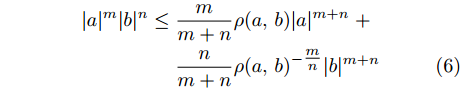
$ a\in {{\bf{R}}} $ ,$ b \in {{\bf{R}}} $ ,$ m\in {{\bf{R}}}_{>0} $ ,$ n\in {{\bf{R}}}_{>0} $ 和函数$ \rho(a,b)>0 $ , 下列不等式成立$$\begin{split} |a|^m|b|^n \le\;& \frac{m}{m+n}\rho(a,b)|a|^{m+n}\;+\\&\frac{n}{m+n}\rho(a,b)^{-\tfrac{m}{n}}|b|^{m+n} \end{split}$$ (6) 引理 3[29-30]. 对任意
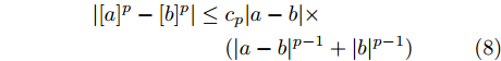
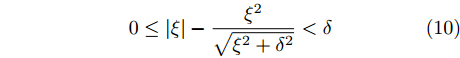
$ p\ge 1 $ ,$ a\in {{\bf{R}}} $ ,$ b \in {{\bf{R}}} $ , 下列不等式成立$$ \|a|^{p}-|b|^{p}|\le |[a]^{p}-[b]^{p}| \hspace{37pt} $$ (7) $$ \begin{split} \,|[a]^{p}-[b]^{p}|\le\; &c_{p}|a-b|\times\\ &(|a-b|^{{p}-1}+|b|^{{p}-1}) \end{split} $$ (8) $$ |a|^{p}+|b|^{p}\le(|a|+|b|)^{p} \hspace{45pt}$$ (9) 其中,
$ c_{p} = 2^{p-2}+2 $ .引理 4[31]. 对任意
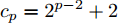
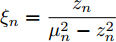
$ \delta\in {{\bf{R}}}_{>0} $ 和$ \xi \in {{\bf{R}}} $ , 下列不等式成立$$ 0\le |\xi|-\frac{\xi^2}{\sqrt{\xi^2+\delta^2}}<\delta $$ (10) 引理 5[32]. 对满足
$ 0\le d<c $ 的$ c\in {{\bf{R}}} $ 和$ d\in {{\bf{R}}} $ , 下列不等式成立$$ \log\frac{c}{c-d} \le \frac{d}{c-d} $$ (11) 2. 自适应跟踪控制策略
本节设计了一种基于障碍李雅普诺夫函数的自适应跟踪控制器, 并给出了闭环系统的稳定性证明.
2.1 自适应控制器设计
定义如下误差坐标变换
$$ z_1 = x_1-y_r $$ (12) $$ z_i = x_i-\alpha_{i-1},\;i = 2,\cdots,n $$ (13) 其中,
$ \alpha_{i-1} $ 是第$ i-1 $ 步的虚拟控制律.步骤
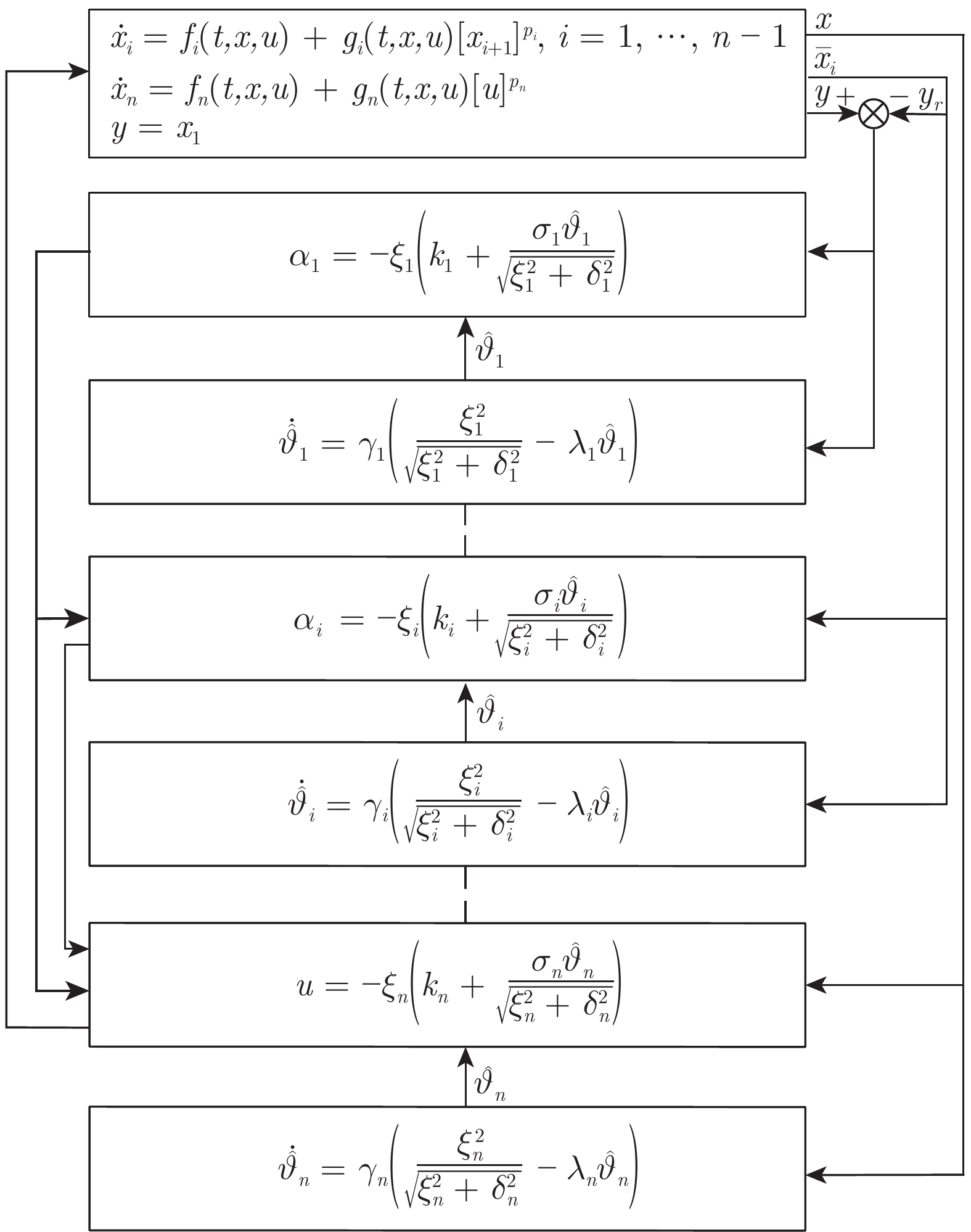
$ {\boldsymbol{i}} $ ${\boldsymbol{(i = 1,\cdots,n-1)}}$ . 选取正常数$ \mu_i $ 满足$ \mu_i>|z_i(0)| $ , 设计第$ i $ 步虚拟控制律和自适应律为$$ \alpha_i = -\xi_i\left(k_i+\frac{\sigma_i\hat{\vartheta}_i}{\sqrt{\xi_i^2+\delta_i^2}}\right) $$ (14) $$ \dot{\hat{\vartheta}}_i = \gamma_i\left(\frac{\xi_i^2}{\sqrt{\xi_i^2+\delta_i^2}}-\lambda_i\hat{\vartheta}_i\right) $$ (15) 其中,
$\xi_i = \dfrac{z_i}{\mu_i^2-z_i^{2}}$ ,$ \hat{\vartheta}_i $ 是$ \vartheta_i $ 的估计值,$ \hat{\vartheta}_i(0)\ge 0 $ ,$ k_i $ ,$ \sigma_i $ ,$ \gamma_i $ 和$ \lambda_i $ 为正常数.步骤 n. 选取正常数
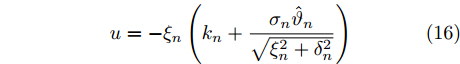
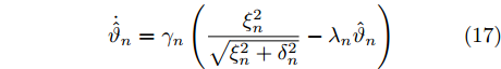
$ \mu_n $ 满足$ \mu_n>|z_n(0)| $ , 设计实际控制律和自适应律为$$ u = -\xi_n\left(k_n+\frac{\sigma_n\hat{\vartheta}_n}{\sqrt{\xi_n^2+\delta_n^2}}\right) $$ (16) $$ \dot{\hat{\vartheta}}_n = \gamma_n\left(\frac{\xi_n^2}{\sqrt{\xi_n^2+\delta_n^2}}-\lambda_n\hat{\vartheta}_n\right) $$ (17) 其中,
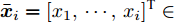
$\xi_n = \dfrac{z_n}{\mu_n^2-z_n^{2}}$ ,$ \hat{\vartheta}_n $ 是$ \vartheta_n $ 的估计值且满足,$\hat{\vartheta}_n(0)\ge 0$ ,$ k_n $ ,$ \sigma_n $ ,$ \gamma_n $ 和$ \lambda_n $ 为正常数.上述自适应控制器的设计过程如图1所示.
注 3. 如式(14) ~ (17)所示, 本文提出的自适应反推控制策略不依赖于系统幂次
$ p_i $ 及其上界信息, 且无需知晓系统函数$ f_i(t,{\boldsymbol{x}},u) $ ,$ g_i(t,{\boldsymbol{x}},u) $ 及相应的界函数$ \bar{f}_{il}(\bar{{\boldsymbol{x}}}_i) $ ,$ \underline{g}_i(\bar{{\boldsymbol{x}}}_{i}) $ ,$ \bar{g}_i(\bar{{\boldsymbol{x}}}_{i}) $ 的解析表达式. 同时, 该控制策略未包含虚拟控制律$ \alpha_i $ 的导数, 消除了积分反推法中“计算膨胀”问题.2.2 稳定性分析
在给出闭环系统的稳定性分析之前, 先引入如下命题.
命题 1. 对式(14) ~ (17)的
$\hat{\vartheta}_1,\cdots,\hat{\vartheta}_n, \alpha_1,\cdots, \alpha_{n-1}$ 和$ u $ , 下列陈述成立i)
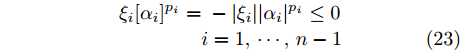
$ \hat{\vartheta}_i(t)\ge 0 $ ,$i = 1,\cdots,n$ .ii)
$\xi_i[\alpha_i]^{p_i} = -|\xi_i||\alpha_i|^{p_i} \le 0, \xi_n [u]^{p_n} = -|\xi_n| |u|^{p_n}$ ,$i = 1,\cdots,n-1$ .证明. i) 由于
$\dfrac{\xi_i^2}{\sqrt{\xi_i^2+\delta_i^2}}\ge 0$ 和$ \hat{\vartheta}_i(0)\ge 0 $ , 根据式(15)和式(17), 可直接推出$ \hat{\vartheta}_i(t)\ge 0 $ ,$i = 1,\cdots,n$ .ii) 根据式(14)和式(16),
$ \alpha_i $ ,$i = 1,\cdots,n-1$ 和$ u $ 改写为$$ \alpha_i = \xi_i\phi_i,i = 1,\cdots,n-1 $$ (18) $$ u = \xi_n\phi_n\hspace{74pt} $$ (19) 其中,
$$ \phi_i = -k_i-\frac{\sigma_i\hat{\vartheta}_i}{\sqrt{\xi_i^2+\delta_i^2}},\;\;i = 1,\cdots,n $$ (20) 从而, 有
$$ \begin{split} \xi_i[\alpha_i]^{p_i} =&\; \xi_i|\alpha_i|^{p_i}{\rm{sign}}(\xi_i\phi_i)\\& \quad i = 1,\cdots,n-1\end{split} $$ (21) $$ \xi_n [u]^{p_n} = \xi_n |u|^{p_n}{\rm{sign}}(\xi_n\phi_n) $$ (22) 另外, 由于
$ \hat{\vartheta}_i(t)\ge 0 $ ,$i = 1,\cdots,n$ , 从式(20)易知$ \phi_i\le 0 $ ,$i = 1,\cdots,n$ , 进而可得${\rm{sign}}(\xi_i\phi_i) = -{\rm{sign}}(\xi_i)$ ,$i = 1,\cdots,n$ . 故$$ \begin{split} \xi_i[\alpha_i]^{p_i} =&\; -|\xi_i||\alpha_i|^{p_i}\le 0\\ & i = 1,\cdots,n-1 \end{split}$$ (23) $$ \xi_n [u]^{p_n} = -|\xi_n| |u|^{p_n}\le 0 $$ (24) □
本文主要结论可总结为如下定理.
定理 1. 对满足假设1和假设2的高阶不确定非线性系统(1), 在任意初始条件
$ {\boldsymbol{x}}(0) $ 下, 控制器(16)以及自适应律(15)和(17)保证了闭环系统的所有信号一致有界, 并且输出跟踪误差可以收敛到残差为任意小的残差集.证明. 本证明共分为3部分. 首先, 证明由系统(1), 控制器(16), 自适应律(15)和(17)组成的闭环系统在最大存在区间
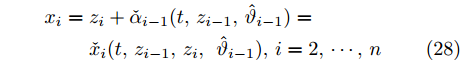
$ [0,t_f) $ 上存在唯一解${\pmb\eta}(t) = [z_1(t),\cdots,z_n(t),\hat{\vartheta}_1(t),\cdots,\hat{\vartheta}_n(t)]^{\rm{T}}$ . 然后, 采用反证法证明$ t_f = +\infty $ . 最后, 实现本文控制目标.Part 1. 根据式(14)和式(16), 虚拟控制律
$\alpha_1,\cdots, \alpha_{n-1}$ , 实际控制律$ u $ 以及系统状态$x_1,\cdots,x_n$ 可写为$$ \alpha_i = \check{\alpha}_i(z_i,\hat{\vartheta}_i),i = 1,\cdots,n-1 $$ (25) $$ u = \check{\alpha}_n(z_n,\hat{\vartheta}_n) $$ (26) $$ x_1 = z_1+y_r= \check{x}_1(t,z_1) $$ (27) $$ \begin{split} x_i =\; & z_i+\check{\alpha}_{i-1}(t,z_{i-1},\hat{\vartheta}_{i-1})=\\ & \check{x}_i(t,z_{i-1},z_i,\;\hat{\vartheta}_{i-1}),i = 2,\cdots,n \end{split} $$ (28) 因此, 由式(1)和式(14)
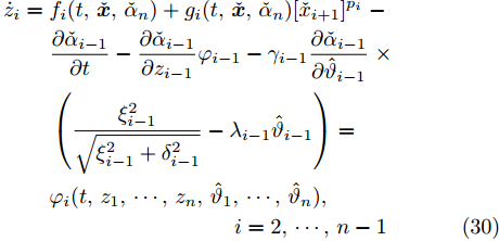
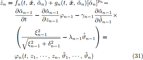
$ \sim $ (17)组成的闭环系统可改写为$$ \begin{split} \dot{z}_1 =\;& f_1(t,\check{{\boldsymbol{x}}},\check{\alpha}_n)+g_1(t,\check{{\boldsymbol{x}}},\check{\alpha}_n)[\check{x}_2]^{p_1}-\dot{y}_r=\\ &\varphi_1(t,z_1,\cdots,z_n,\hat{\vartheta}_1,\cdots,\hat{\vartheta}_n) \end{split} $$ (29) $$ \begin{split} \dot{z}_i = \;& f_i(t,\check{{\boldsymbol{x}}},\check{\alpha}_n)+g_i(t,\check{{\boldsymbol{x}}},\check{\alpha}_n)[\check{x}_{i+1}]^{p_i}\;-\\ &\frac{\partial \check{\alpha}_{i-1}}{\partial t}-\frac{\partial \check{\alpha}_{i-1}}{\partial z_{i-1}}\varphi_{i-1}-\gamma_{i-1}\frac{\partial \check{\alpha}_{i-1}}{\partial \hat{\vartheta}_{i-1}}\;\times\\ &\left(\frac{\xi_{i-1}^2}{\sqrt{\xi_{i-1}^2+\delta_{i-1}^2}}-\lambda_{i-1}\hat{\vartheta}_{i-1}\right)=\\ & \varphi_i(t,z_1,\cdots,z_n,\hat{\vartheta}_1,\cdots,\hat{\vartheta}_n),\\ &\qquad\qquad\qquad\qquad\;\; i = 2,\cdots,n-1 \end{split}$$ (30) $$ \begin{split} \dot{z}_n =\; &f_n(t,\check{{\boldsymbol{x}}},\check{\alpha}_n)+g_n(t,\check{{\boldsymbol{x}}},\check{\alpha}_n)[\check{\alpha}_n]^{p_n}-\\ &\frac{\partial \check{\alpha}_{n-1}}{\partial t}-\frac{\partial \check{\alpha}_{n-1}}{\partial z_{n-1}}\varphi_{n-1}-\gamma_{n-1}\frac{\partial \check{\alpha}_{n-1}}{\partial \hat{\vartheta}_{n-1}}\times\\ &\left(\frac{\xi_{n-1}^2}{\sqrt{\xi_{n-1}^2+\delta_{n-1}^2}}-\lambda_{n-1}\hat{\vartheta}_{n-1}\right)=\\& \varphi_n(t,z_1,\cdots,z_n,\hat{\vartheta}_1,\cdots,\hat{\vartheta}_n) \end{split}$$ (31) $$ \begin{split} \dot{\hat{\vartheta}}_i =\;& \gamma_i\Big(\frac{\xi_i^2}{\sqrt{\xi_i^2+\delta_i^2}}-\lambda_i\hat{\vartheta}_i\Big)=\\ & \varphi_{n+i}(t,z_i,\hat{\vartheta}_i),\;\;i = 1,\cdots,n \end{split} $$ (32) 其中,
$\check{{\boldsymbol{x}}} = [\check{x}_1,\cdots,\check{x}_n]^{\rm{T}}\in {{\bf{R}}}^n$ .定义开集
$$ \Xi = \underbrace{(-\mu_1,\mu_1)\times\cdots\times(-\mu_n,\mu_n)}_n\times {{\bf{R}}}^n $$ 由于
$\mu_i > |z_i(0)|$ ,$i = 1,\cdots,n$ , 可知${\boldsymbol{\eta}}(0) = [z_1(0), \cdots, z_n(0),\hat{\vartheta}_1(0),\cdots,\hat{\vartheta}_n(0)]^{\rm{T}}\in \Xi$ . 同时, 由于期望参考信号$ y_r $ 及其导数$ \dot{y}_r $ 有界, 函数$ f_i, g_i $ ,$i = 1,\cdots, n$ 在$ t $ 上分段连续, 且关于$ {\boldsymbol{x}} $ 和$ u $ 满足局部Lipschitz条件, 可推得$ \varphi_i:{{\bf{R}}}_{\ge0}\times \Xi\rightarrow {{\bf{R}}} $ 在$ t $ 上分段连续, 且关于$ {\boldsymbol{x}} $ 和$ u $ 满足局部Lipschitz条件. 根据微分方程解的存在唯一性定理[33], 对任意初始条件$ {\boldsymbol{\eta}}(0) $ , 闭环系统(29) ~ (32)在最大存在区间$ [0,t_f) $ 上存在唯一解${\boldsymbol{\eta}} = [z_1,\cdots,z_n,\hat{\vartheta}_1,\cdots,\hat{\vartheta}_n]^{\rm{T}}\in \Xi$ , 即, 对$\forall t\in [0,t_f)$ ,$ |z_i|<\mu_i $ ,$i = 1,\cdots,n$ .Part 2. 本部分采用反证法证明
$ t_f = +\infty $ . 为此, 不妨假设$ t_f<+\infty $ .考虑如下障碍李雅普诺夫函数[26]:
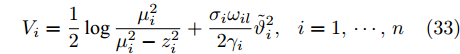
$$ V_i = \frac{1}{{2}}\log\frac{\mu_i^2}{\mu_i^2-z_i^{2}}+\frac{\sigma_i\omega_{il} }{2\gamma_i}\tilde{\vartheta}_i^2,\;\;i = 1,\cdots,n $$ (33) 其中,
$ \tilde{\vartheta}_i = \vartheta_i-\hat{\vartheta}_i $ ,$ \omega_{il} $ 是未知正常数.步骤
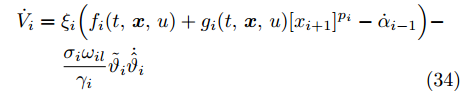
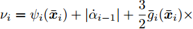
$ {\boldsymbol{i}} $ ${\boldsymbol{(i = 1,\cdots,n-1)}}$ .$ V_i $ 的导数为$$ \begin{split} \dot{V}_i = \;&\xi_i\Big(f_i(t,{\boldsymbol{x}},u)+g_i(t,{\boldsymbol{x}},u)[x_{i+1}]^{p_i}-\dot{\alpha}_{i-1}\Big)-\\ &\frac{\sigma_i\omega_{il} }{\gamma_i}\tilde{\vartheta}_i\dot{\hat{\vartheta}}_i \\[-10pt]\end{split}$$ (34) 其中,
$ \alpha_0 = y_r $ .根据假设1和引理2, 下列不等式成立
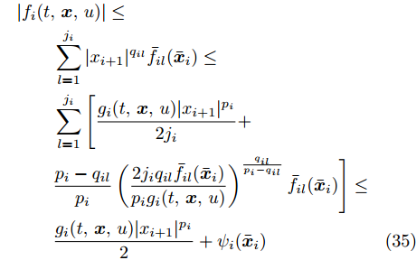
$$ \begin{split} &|f_i(t,{\boldsymbol{x}},u)|\le\\ &\qquad\sum\limits_{l = 1}^{j_i}|x_{i+1}|^{q_{il}}\bar{f}_{il}(\bar{{\boldsymbol{x}}}_i)\le\\ &\qquad\sum\limits_{l = 1}^{j_i}\Bigg[\frac{g_i(t,{\boldsymbol{x}},u)|x_{i+1}|^{p_i}}{2j_i}+\\ &\qquad\frac{p_i-q_{il}}{p_i}\left(\frac{2j_iq_{il}\bar{f}_{il}(\bar{{\boldsymbol{x}}}_i)}{p_ig_i(t,{\boldsymbol{x}},u)}\right)^{\frac{q_{il}}{p_i-q_{il}}}\bar{f}_{il}(\bar{{\boldsymbol{x}}}_i)\Bigg]\le\\ &\qquad\frac{g_i(t,{\boldsymbol{x}},u)|x_{i+1}|^{p_i}}{2}+\psi_i(\bar{{\boldsymbol{x}}}_i) \end{split} $$ (35) 其中,
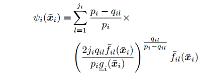
$$ \begin{split} \psi_i(\bar{{\boldsymbol{x}}}_i) =& \sum\limits_{l = 1}^{j_i}\frac{p_i-q_{il}}{p_i}\times\\ &\left(\frac{2j_iq_{il}\bar{f}_{il}(\bar{{\boldsymbol{x}}}_i)}{p_i\underline{g}_i(\bar{{\boldsymbol{x}}}_i)}\right)^{\tfrac{q_{il}}{p_i-q_{il}}}\bar{f}_{il}(\bar{{\boldsymbol{x}}}_i) \end{split}$$ 将式(35)代入式(34), 可得
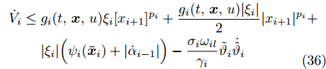
$$ \begin{split} \dot{V}_i\le\; &g_i(t,{\boldsymbol{x}},u)\xi_i [x_{i+1}]^{p_i}+\frac{g_i(t,{\boldsymbol{x}},u)|\xi_i|}{2}|x_{i+1}|^{p_i}+\\& |\xi_i|\Big(\psi_i(\bar{{\boldsymbol{x}}}_i)+|\dot{\alpha}_{i-1}|\Big)-\frac{\sigma_i\omega_{il} }{\gamma_i}\tilde{\vartheta}_i\dot{\hat{\vartheta}}_i \\[-10pt]\end{split}$$ (36) 根据命题1, 可得
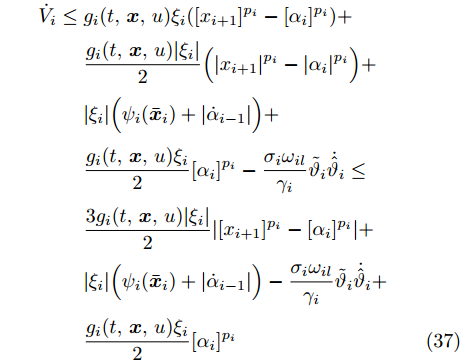
$$ \begin{split} \dot{V}_i\le \;&g_i(t,{\boldsymbol{x}},u)\xi_{i}([x_{i+1}]^{p_i}-[\alpha_{i}]^{p_i})+\\ &\frac{g_i(t,{\boldsymbol{x}},u)|\xi_i|}{2}\Big(|x_{i+1}|^{p_i}-|\alpha_{i}|^{p_i}\Big)+\\ &|\xi_i|\Big(\psi_i(\bar{{\boldsymbol{x}}}_i)+|\dot{\alpha}_{i-1}|\Big)+\\ &\frac{g_i(t,{\boldsymbol{x}},u)\xi_{i}}{2}[\alpha_i]^{p_i}-\frac{\sigma_i\omega_{il} }{\gamma_i}\tilde{\vartheta}_i\dot{\hat{\vartheta}}_i\le\\ &\frac{3g_i(t,{\boldsymbol{x}},u)|\xi_i|}{2}|[x_{i+1}]^{p_i}-[\alpha_{i}]^{p_i}|+\\ &|\xi_i|\Big(\psi_i(\bar{{\boldsymbol{x}}}_i)+|\dot{\alpha}_{i-1}|\Big)-\frac{\sigma_i\omega_{il} }{\gamma_i}\tilde{\vartheta}_i\dot{\hat{\vartheta}}_i+\\& \frac{g_i(t,{\boldsymbol{x}},u)\xi_{i}}{2}[\alpha_i]^{p_i} \end{split}$$ (37) 为了处理式(37)中的项
$ |\xi_i||[x_{i+1}]^{p_i}-[\alpha_{i}]^{p_i}| $ , 考虑以下两种情形.情形 1. 当
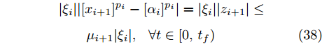
$ p_i = 1 $ 时. 由Part 1可得:$|z_{i+1}| < \mu_{i+1}$ ,$ \forall t\in [0,t_f) $ , 因而$$ \begin{split} &|\xi_i||[x_{i+1}]^{p_i}-[\alpha_{i}]^{p_i}|= |\xi_i||z_{i+1}|\le\\ &\qquad \mu_{i+1}|\xi_i|, \;\;\forall t\in [0,t_f) \end{split} $$ (38) 情形 2. 当
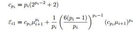
$ p_i>1 $ 时. 由引理2和引理3以及$|z_{i+1}| < \mu_{i+1}$ ,$ \forall t\in [0,t_f) $ , 可得$$\begin{split} &|\xi_i||[x_{i+1}]^{p_i}-[\alpha_{i}]^{p_i}|=\\ &\quad\; \; \; \; |\xi_i||[z_{i+1}+\alpha_{i}]^{p_i}-[\alpha_{i}]^{p_i}|\le\\ &\quad\; \; \; \; c_{p_i}|\xi_i|(\mu_{i+1}^{p_i}+\mu_{i+1}|\alpha_i|^{p_i-1})\le\\ &\quad\; \; \; \; |\xi_i|\Big(\frac{|\alpha_i|^{p_i}}{6}+\bar{\varepsilon}_{i1}\Big),\;\;\forall t\in [0,t_f) \end{split}$$ (39) 其中,
$$ \begin{split} &c_{p_i} = p_i(2^{p_i-2}+2)\\ &\bar{\varepsilon}_{i1} = c_{p_i}\mu_{i+1}^{p_i}+\frac{1}{p_i}\left(\frac{6(p_i-1)}{p_i}\right)^{p_i-1}(c_{p_i}\mu_{i+1})^{p_i} \end{split}$$ 综合情形1和情形2, 项
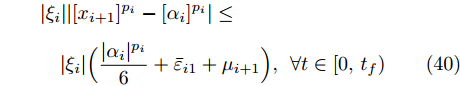
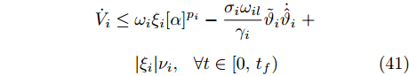
$ |\xi_i||[x_{i+1}]^{p_i}-[\alpha_{i}]^{p_i}| $ 放缩为$$ \begin{split} &|\xi_i||[x_{i+1}]^{p_i}-[\alpha_{i}]^{p_i}| \le\\ &\quad|\xi_i|\Big(\frac{|\alpha_i|^{p_i}}{6}+\bar{\varepsilon}_{i1}+\mu_{i+1}\Big),\;\forall t\in [0,t_f) \end{split} $$ (40) 将式(40)代入式(37)中, 并结合命题1, 易得
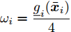
$$ \begin{split} \dot{V}_i\le\;&\omega_i\xi_{i}[\alpha]^{p_i}-\frac{\sigma_i\omega_{il} }{\gamma_i}\tilde{\vartheta}_i\dot{\hat{\vartheta}}_i\;+\\ &|\xi_i|\nu_i,\;\;\forall t\in [0,t_f) \end{split} $$ (41) 其中,
$\omega_i = \dfrac{\underline{g}_i(\bar{{\boldsymbol{x}}}_i)}{4}$ ,$\nu_i = \psi_i(\bar{{\boldsymbol{x}}}_i)+|\dot{\alpha}_{i-1}|+\dfrac{3}{2}\bar{g}_i(\bar{{\boldsymbol{x}}}_{i})\times (\bar{\varepsilon}_{i1}+ \mu_{i+1})$ .由Part 1可知, 对
$ \forall t\in [0,t_f) $ ,$ |z_j|<\mu_j $ ,$j = 1, \cdots, i$ . 同时, 依据假设1和假设2,$ y_r $ ,$ \dot{y}_r $ 有界, 且$ \bar{f}_{il} $ ,$ \underline{g}_i $ 和$ \bar{g}_i $ 为连续函数. 此外, 根据第$ i-1 $ 步设计, 可推知$x_1,\cdots,x_i$ ,$ \dot{\alpha}_{i-1} $ 有界,$ \forall t\in [0,t_f) $ . 因此, 运用极值定理, 对$ \forall t\in [0,t_f) $ , 有$$ 0< \omega_{il}\le \omega_i \, $$ (42) $$ 0\le \nu_i\le \nu_{im} $$ (43) 其中,
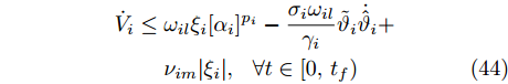
$ \omega_{il} $ 和$ \nu_{im} $ 为未知正常数.将式(42)和式(43)代入式(41)中, 有
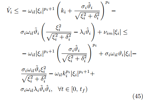
$$ \begin{split} \dot{V}_i\le\;&\omega_{il}\xi_{i}[\alpha_i]^{p_i}-\frac{\sigma_i\omega_{il} }{\gamma_i}\tilde{\vartheta}_i\dot{\hat{\vartheta}}_i+\\ &\nu_{im}|\xi_i|,\;\;\forall t\in [0,t_f) \end{split} $$ (44) 通过式(14)和式(15), 并结合引理3, 可得
$$ \begin{split} \dot{V}_i\le\;&-\omega_{il}|\xi_{i}|^{p_i+1}\left(k_i+\frac{\sigma_i\hat{\vartheta}_i}{\sqrt{\xi_i^2+\delta_i^2}}\right)^{p_i}-\\& \sigma_i\omega_{il} \tilde{\vartheta}_i\left(\frac{\xi_i^2}{\sqrt{\xi_i^2+\delta_i^2}}-\lambda_i\hat{\vartheta}_i\right)+\nu_{im}|\xi_i|\le\\ &-\omega_{il} |\xi_{i}|^{p_i+1}\left(\frac{\sigma_i\hat{\vartheta}_i}{\sqrt{\xi_i^2+\delta_i^2}}\right)^{p_i}+\sigma_i\omega_{il} \vartheta_i|\xi_i|-\\ &\frac{\sigma_i\omega_{il} \tilde{\vartheta}_i\xi_i^2}{\sqrt{\xi_i^2+\delta_i^2}}-\omega_{il} k_i^{p_i}|\xi_{i}|^{p_i+1}+\\ &\sigma_i\omega_{il} \lambda_i\tilde{\vartheta}_i\hat{\vartheta}_i,\;\;\forall t\in [0,t_f) \end{split} $$ (45) 其中,
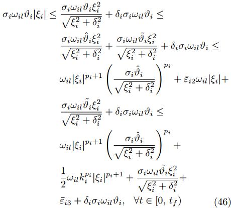
$\vartheta_i = \dfrac{\nu_{im}}{\sigma_i\omega_{il}}$ .根据引理2和引理4, 式(45)中的项
$ \sigma_i\omega_{il}\vartheta_i|\xi_i| $ 放缩为$$ \begin{split} \sigma_i\omega_{il} \vartheta_i|\xi_i|\le\;&\frac{\sigma_i\omega_{il} \vartheta_i\xi_i^2}{\sqrt{\xi_i^2+\delta_i^2}}+\delta_i\sigma_i\omega_{il} \vartheta_i\le\\ &\frac{\sigma_i\omega_{il} \hat{\vartheta}_i\xi_i^2}{\sqrt{\xi_i^2+\delta_i^2}}+\frac{\sigma_i\omega_{il} \tilde{\vartheta_i}\xi_i^2}{\sqrt{\xi_i^2+\delta_i^2}}+\delta_i\sigma_i\omega_{il} \vartheta_i\le\\& \omega_{il} |\xi_{i}|^{p_i+1}\left(\frac{\sigma_i\hat{\vartheta}_i}{\sqrt{\xi_i^2+\delta_i^2}}\right)^{p_i}+\bar{\varepsilon}_{i2}\omega_{il} |\xi_i|+\\ &\frac{\sigma_i\omega_{il} \tilde{\vartheta_i}\xi_i^2}{\sqrt{\xi_i^2+\delta_i^2}}+\delta_i\sigma_i\omega_{il} \vartheta_i\le\\ & \omega_{il} |\xi_{i}|^{p_i+1}\left(\frac{\sigma_i\hat{\vartheta}_i}{\sqrt{\xi_i^2+\delta_i^2}}\right)^{p_i}+\\ &\frac{1}{2}\omega_{il} k_i^{p_i}|\xi_{i}|^{p_i+1}+\frac{\sigma_i\omega_{il} \tilde{\vartheta_i}\xi_i^2}{\sqrt{\xi_i^2+\delta_i^2}}+\\ &\bar{\varepsilon}_{i3}+\delta_i\sigma_i\omega_{il} \vartheta_i,\;\;\forall t\in [0,t_f) \\[-10pt]\end{split} $$ (46) 其中,
$$ \begin{split} &{{\bar \varepsilon }_{i2}} = \left\{ {\begin{array}{*{20}{l}} {0,}&{{p_i} = 1}\\ {\dfrac{{{p_i} - 1}}{{{p_i}}}{{\left(\dfrac{1}{{{p_i}}}\right)}^{\tfrac{1}{{{p_i} - 1}}}},}&{{p_i} > 1} \end{array}} \right.\\ &{{\bar \varepsilon }_{i3}} = \left\{ {\begin{array}{*{20}{l}} {0,}&{{{\bar \varepsilon }_{i2}} = 0}\\ {\dfrac{{{{\bar \varepsilon }_{i2}}{\omega _{il}}{p_i}}}{{{p_i} + 1}}{{\left(\dfrac{{2{{\bar \varepsilon }_{i2}}}}{{k_i^{{p_i}}({p_i} + 1)}}\right)}^{\tfrac{1}{{{p_i}}}}}},&{{{\bar \varepsilon }_{i2}} > 0} \end{array}} \right. \end{split}$$ 由式(45)和式(46), 可得
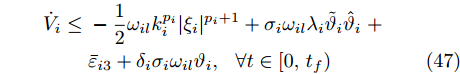
$$\begin{split} \dot{V}_i\le\; &-\frac{1}{2}\omega_{il} k_i^{p_i}|\xi_{i}|^{p_i+1}+\sigma_i\omega_{il} \lambda_i\tilde{\vartheta}_i\hat{\vartheta}_i\;+\\ &\bar{\varepsilon}_{i3}+\delta_i\sigma_i\omega_{il} \vartheta_i,\;\;\forall t\in [0,t_f) \end{split} $$ (47) 依据引理2和引理5, 以及Young不等式, 则有
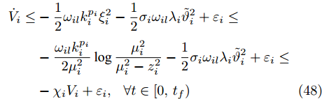
$$ \begin{split} \dot{V}_i\le&-\frac{1}{2}\omega_{il} k_i^{p_i}\xi_{i}^2-\frac{1}{2}\sigma_i\omega_{il} \lambda_i\tilde{\vartheta}_i^2+\varepsilon_i\le\\ &-\frac{\omega_{il} k_i^{p_i}}{2\mu_i^2}\log\frac{\mu_i^2}{\mu_i^2-z_i^{2}}-\frac{1}{2}\sigma_i\omega_{il} \lambda_i\tilde{\vartheta}_i^2+\varepsilon_i\le\\ &-\chi_iV_i+\varepsilon_i,\;\;\forall t\in [0,t_f) \end{split}$$ (48) 其中,
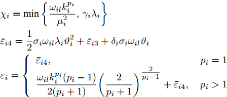
$$ \begin{split} &{\chi _i} = \min \left\{ \frac{{{\omega _{il}}k_i^{{p_i}}}}{{\mu _i^2}},{\gamma _i}{\lambda _i}\right\} \\ &{{\bar \varepsilon }_{i4}} = \frac{1}{2}{\sigma _i}{\omega _{il}}{\lambda _i}\vartheta _i^2 + {{\bar \varepsilon }_{i3}} + {\delta _i}{\sigma _i}{\omega _{il}}{\vartheta _i}\\ &{\varepsilon _i} = \left\{ \begin{array}{*{20}{l}} {{{\bar \varepsilon }_{i4}},}&{{p_i} = 1}\\ {\dfrac{{{\omega _{il}}k_i^{{p_i}}({p_i} - 1)}}{{2({p_i} + 1)}}{{\left(\dfrac{2}{{{p_i} + 1}}\right)}^{\tfrac{2}{{{p_i} - 1}}}} + {{\bar \varepsilon }_{i4}},}&{{p_i} > 1} \end{array} \right. \end{split} $$ 因此, 存在正常数
$ \chi_i^* $ 和$ \varepsilon_i^* $ 满足$$ 0<\chi_i^*\le\chi_i $$ (49) $$ 0<\varepsilon_i\le\varepsilon_i^* $$ (50) 由式(48) ~ (50), 可得
$$ \dot{V}_i\le-\chi_i^*V_i+\varepsilon_i^*,\;\forall t\in [0,t_f) $$ (51) 因此, 对
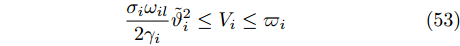
$ \forall t\in [0,t_f) $ 中, 有$$ \frac{1}{2}\log\frac{\mu_i^2}{\mu_i^2-z_i^{2}}\le V_i\le \varpi_i $$ (52) $$ \frac{\sigma_i\omega_{il} }{2\gamma_i}\tilde{\vartheta}_i^2\le V_i\le \varpi_i\;\; \qquad $$ (53) 其中,
$\varpi_i = \max\{V_i(0),\dfrac{\varepsilon_i^*}{\chi_i^*}\}$ .从式(52)和式(53), 可得
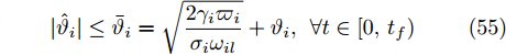
$$ |z_i|\le\bar{\mu}_i = \mu_i\sqrt{1-\exp(-{2}\varpi_i)}<\mu_i $$ (54) $$ |\hat{\vartheta}_i|\le\bar{\vartheta}_i = \sqrt{\frac{2\gamma_i\varpi_i}{\sigma_i\omega_{il}}}+\vartheta_i,\;\forall t\in [0,t_f) $$ (55) 进而可推出, 对
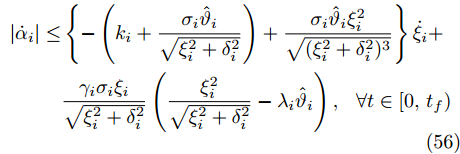
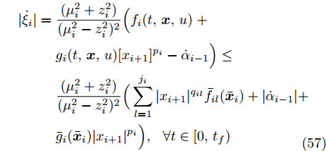
$ \forall t\in [0,t_f) $ ,$ \alpha_i $ 和$ x_{i+1} $ 有界. 接着, 对$ \alpha_i $ 和$ \xi_i $ 分别求导, 可得$$ \begin{split}|\dot{\alpha}_i|\le&\left\{-\left(k_i+\frac{\sigma_i\hat{\vartheta}_i}{\sqrt{\xi_i^2+\delta_i^2}}\right)+\frac{\sigma_i\hat{\vartheta}_i\xi_i^2}{\sqrt{(\xi_i^2+\delta_i^2)^3}}\right\}\dot{\xi}_i+\\ & \frac{\gamma_i\sigma_i\xi_i}{\sqrt{\xi_i^2+\delta_i^2}}\left(\frac{\xi_i^2}{\sqrt{\xi_i^2+\delta_i^2}} -\lambda_i\hat{\vartheta}_i\right),\;\;\forall t\in [0,t_f) \end{split}$$ (56) $$ \begin{split} |\dot{\xi}_i| =\; &\frac{(\mu_i^2+z_i^2)}{(\mu_i^2-z_i^2)^2}\Big(f_i(t,{\boldsymbol{x}},u)\;+\\ &g_i(t,{\boldsymbol{x}},u)[x_{i+1}]^{p_i}-\dot{\alpha}_{i-1}\Big)\le\\ &\frac{(\mu_i^2+z_i^2)}{(\mu_i^2-z_i^2)^2}\Big(\sum\limits_{l = 1}^{j_i}|x_{i+1}|^{q_{il}}\bar{f}_{il}(\bar{{\boldsymbol{x}}}_i)+|\dot{\alpha}_{i-1}|+\\ &\bar{g}_i(\bar{{\boldsymbol{x}}}_{i})|x_{i+1}|^{p_i}\Big),\;\;\forall t\in [0,t_f)\\[-10pt] \end{split} $$ (57) 从式(56)和式(57)可知, 对
$ \forall t\in [0,t_f) $ ,$ \dot{\xi}_i $ 和$ \dot{\alpha}_i $ 亦有界.步骤
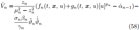
$ {\boldsymbol{n}} $ . 求$ V_n $ 的导数, 可得$$ \begin{split} \dot{V}_n =& \frac{z_n}{\mu_n^2-z_n^{2}}(f_n(t,{\boldsymbol{x}},u) + g_n(t,{\boldsymbol{x}},u)[u]^{p_n}-\dot{\alpha}_{n-1})-\\ &\frac{\sigma_n\beta_n}{\gamma_n}\tilde{\vartheta}_n\dot{\hat{\vartheta}}_n \\[-10pt]\end{split}$$ (58) 类似于式(35)的推导过程, 利用假设1和引理2, 可得
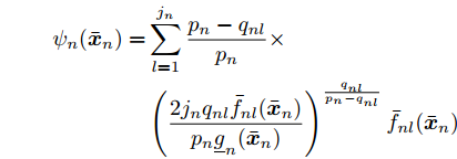
$$ |f_n(t,{\boldsymbol{x}},u)|\le \frac{1}{2}g_n(t,{\boldsymbol{x}},u)|u|^{p_n}+\psi_n(\bar{{\boldsymbol{x}}}_n) $$ (59) 其中,
$$ \begin{split} \psi_n(\bar{{\boldsymbol{x}}}_n) = &\sum\limits_{l = 1}^{j_n}\frac{p_n-q_{nl}}{p_n}\times\\ &\left(\frac{2j_nq_{nl}\bar{f}_{nl}(\bar{{\boldsymbol{x}}}_n)}{p_n\underline{g}_n(\bar{{\boldsymbol{x}}}_n)}\right)^{\frac{q_{nl}}{p_n-q_{nl}}}\bar{f}_{nl}(\bar{{\boldsymbol{x}}}_n) \end{split}$$ 由式(59)以及命题1, 可推得
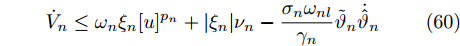
$$ \dot{V}_n\le\omega_n\xi_n[u]^{p_n}+|\xi_n|\nu_n-\frac{\sigma_n\omega_{nl} }{\gamma_n}\tilde{\vartheta}_n\dot{\hat{\vartheta}}_n $$ (60) 其中,
$\omega_n = \dfrac{\underline{g}_n(\bar{{\boldsymbol{x}}}_n)}{2}$ ,$ \nu_n = \psi_n(\bar{{\boldsymbol{x}}}_n)+|\dot{\alpha}_{n-1}| $ .由Part 1可知, 对
$ \forall t\in [0,t_f) $ ,$ |z_j|<\mu_j $ ,$j = 1, \cdots, n$ . 同时, 根据假设1和假设2,$ y_r $ 和$ \dot{y}_r $ 有界, 且$ \bar{f}_{nl} $ ,$ \underline{g}_n $ 和$ \bar{g}_n $ 连续. 此外, 由第$ n-1 $ 步设计可推得$x_1,\cdots, x_n$ ,$ \dot{\alpha}_{n-1} $ 有界,$ \forall t\in [0,t_f) $ . 因此, 运用极值定理, 对$ \forall t\in [0,t_f) $ , 有$$ 0< \omega_{nl}\le \omega_n $$ (61) $$ 0\le \nu_n\le \nu_{nm} $$ (62) 其中,
$ \omega_{nl} $ 和$ \nu_{nm} $ 为未知正常数.利用式(61)和式(62), 有
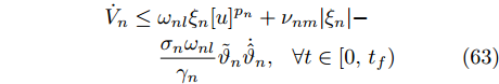
$$ \begin{split} \dot{V}_n\le\;&\omega_{nl}\xi_n[u]^{p_n}+\nu_{nm}|\xi_n|-\\& \frac{\sigma_n\omega_{nl} }{\gamma_n}\tilde{\vartheta}_n\dot{\hat{\vartheta}}_n,\;\;\forall t\in [0,t_f) \end{split} $$ (63) 根据式(16)和式(17)以及命题1和引理3, 可得
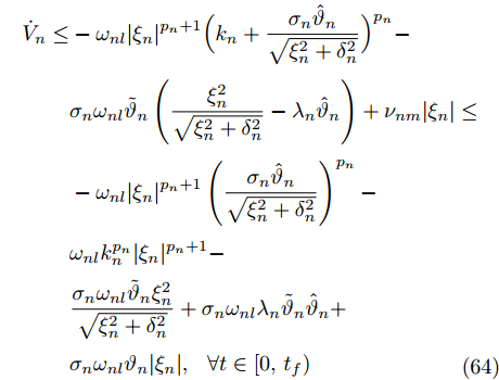
$$ \begin{split} \dot{V}_n\le&-\omega_{nl}|\xi_{n}|^{p_n+1}\Big(k_n+\frac{\sigma_n\hat{\vartheta}_n}{\sqrt{\xi_n^2+\delta_n^2}}\Big)^{p_n}-\\ &\sigma_n\omega_{nl} \tilde{\vartheta}_n\left(\frac{\xi_n^2}{\sqrt{\xi_n^2+\delta_n^2}}-\lambda_n\hat{\vartheta}_n\right)+\nu_{nm}|\xi_n|\le\\ & -\omega_{nl} |\xi_{n}|^{p_n+1}\left(\frac{\sigma_n\hat{\vartheta}_n}{\sqrt{\xi_n^2+\delta_n^2}}\right)^{p_n}-\\ &\omega_{nl} k_n^{p_n}|\xi_{n}|^{p_n+1}-\\ &\frac{\sigma_n\omega_{nl} \tilde{\vartheta}_n\xi_n^2}{\sqrt{\xi_n^2+\delta_n^2}}+\sigma_n\omega_{nl} \lambda_n\tilde{\vartheta}_n\hat{\vartheta}_n+\\ &\sigma_n\omega_{nl} \vartheta_n|\xi_n|,\;\;\forall t\in [0,t_f) \\[-10pt]\end{split}$$ (64) 其中,
$\vartheta_n = \dfrac{\nu_{nm}}{\sigma_n\omega_{nl}}$ .依据引理2和引理4, 式(64)中的项
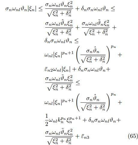
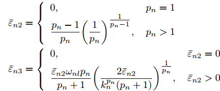
$ \sigma_n\omega_{nl}\vartheta_n|\xi_n| $ 放缩为$$ \begin{split} \sigma_n\omega_{nl} \vartheta_n|\xi_n|\le\;&\frac{\sigma_n\omega_{nl} \vartheta_n\xi_n^2}{\sqrt{\xi_n^2+\delta_n^2}}+\delta_n\sigma_n\omega_{nl} \vartheta_n\le\\ & \frac{\sigma_n\omega_{nl} \hat{\vartheta}_n\xi_n^2}{\sqrt{\xi_n^2+\delta_n^2}}+\frac{\sigma_n\omega_{nl} \tilde{\vartheta}_n\xi_n^2}{\sqrt{\xi_n^2+\delta_n^2}}\;+\\ &\delta_n\sigma_n\omega_{nl} \vartheta_n\le\\ &\omega_{nl} |\xi_n|^{p_n+1}\left(\frac{\sigma_n\hat{\vartheta}_n}{\sqrt{\xi_n^2+\delta_n^2}}\right)^{p_n}+\\ &\bar{\varepsilon}_{n2}\omega_{nl} |\xi_n|+\delta_n\sigma_n\omega_{nl}\vartheta_n+\\ &\frac{\sigma_n\omega_{nl} \tilde{\vartheta}_n\xi_n^2}{\sqrt{\xi_n^2+\delta_n^2}}\le\\ &\omega_{nl} |\xi_n|^{p_n+1}\left(\frac{\sigma_n\hat{\vartheta}_n}{\sqrt{\xi_n^2+\delta_n^2}}\right)^{p_n}+\\ &\frac{1}{2}\omega_{nl} k_n^{p_n}\xi_{n}^{p_n+1}+\delta_n\sigma_n\omega_{nl} \vartheta_n+\\ &\frac{\sigma_n\omega_{nl}\tilde{\vartheta}_n\xi_n^2}{\sqrt{\xi_n^2+\delta_n^2}}+\bar{\varepsilon}_{n3} \end{split} $$ (65) 其中,
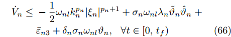
$$ \begin{split} &{{\bar \varepsilon }_{n2}} = \left\{ {\begin{array}{*{20}{l}} {0,}&{{p_n} = 1}\\ {\dfrac{{{p_n} - 1}}{{{p_n}}}{{\left(\dfrac{1}{{{p_n}}}\right)}^{\tfrac{1}{{{p_n} - 1}}}},}&{{p_n} > 1} \end{array}} \right.\\ &{{\bar \varepsilon }_{n3}} = \left\{ {\begin{array}{*{20}{l}} {0,}&{{{\bar \varepsilon }_{n2}} = 0}\\ {\dfrac{{{{\bar \varepsilon }_{n2}}{\omega _{nl}}{p_n}}}{{{p_n} + 1}}{{\left(\dfrac{{2{{\bar \varepsilon }_{n2}}}}{{k_n^{{p_n}}({p_n} + 1)}}\right)}^{\tfrac{1}{{{p_n}}}}},}&{{{\bar \varepsilon }_{n2}} > 0} \end{array}} \right. \end{split} $$ 将式(65)代入式(64)中, 得到
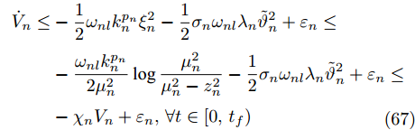
$$ \begin{split} \dot{V}_n\le\;&-\frac{1}{2}\omega_{nl} k_n^{p_n}|\xi_{n}|^{p_n+1}+\sigma_n\omega_{nl} \lambda_n\tilde{\vartheta}_n\hat{\vartheta}_n\;+\\ &\bar{\varepsilon}_{n3}+\delta_n\sigma_n\omega_{nl} \vartheta_n,\;\;\forall t\in [0,t_f) \end{split} $$ (66) 根据引理2和引理5, 以及Young不等式, 可得
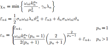
$$ \begin{split} \dot{V}_n\le&-\frac{1}{2}\omega_{nl} k_n^{p_n}\xi_{n}^2-\frac{1}{2}\sigma_n\omega_{nl} \lambda_n\tilde{\vartheta}_n^2+\varepsilon_n\le\\ &-\frac{\omega_{nl} k_n^{p_n}}{2\mu_n^2}\log\frac{\mu_n^2}{\mu_n^2-z_n^{2}}-\frac{1}{2}\sigma_n\omega_{nl} \lambda_n\tilde{\vartheta}_n^2+\varepsilon_n\le\\ &-\chi_nV_n+\varepsilon_n,\forall t\in [0,t_f) \\[-10pt]\end{split} $$ (67) 其中,
$$ \begin{split} &{\chi _n} = \min \left\{ \frac{{{\omega _{nl}}k_n^{{p_n}}}}{{\mu _n^2}},{\gamma _n}{\lambda _n}\right\} \\ &{{\bar \varepsilon }_{n4}} = \frac{1}{2}{\sigma _n}{\omega _{nl}}{\lambda _n}\vartheta _n^2 + {{\bar \varepsilon }_{n3}} + {\delta _n}{\sigma _n}{\omega _{nl}}{\vartheta _n}\\ &{\varepsilon _n} = \left\{ {\begin{array}{*{20}{l}} {{{\bar \varepsilon }_{n4}},}&{{p_n} = 1}\\ {\dfrac{{{\omega _{nl}}k_n^{{p_n}}({p_n} - 1)}}{{2({p_n} + 1)}}{{\left(\dfrac{2}{{{p_n} + 1}}\right)}^{\tfrac{2}{{{p_n} - 1}}}} + {{\bar \varepsilon }_{n4}},}&{{p_n} > 1} \end{array}} \right. \end{split} $$ 因此, 存在正常数
$ \chi_n^* $ 和$ \varepsilon_n^* $ , 使得$$ 0<\chi_n^*\le \chi_n $$ (68) $$ 0<\varepsilon_n\le\varepsilon_n^* \; $$ (69) 根据式(67) ~ (69), 可得
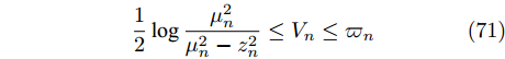
$$ \dot{V}_n\le-\chi_n^*V_n+\varepsilon_n^*,\;\;\forall t\in [0,t_f) $$ (70) 因此, 对
$ \forall t\in [0,t_f) $ , 有$$ \frac{1}{2}\log\frac{\mu_n^2}{\mu_n^2-z_n^{2}}\le V_n\le \varpi_n $$ (71) $$ \frac{\sigma_n\omega_{nl} }{2\gamma_n}\tilde{\vartheta}_n^2\le V_n\le \varpi_n\;\;\;\;\;\;\; $$ (72) 其中,
$\varpi_n = \max\{V_n(0),\dfrac{\varepsilon_n^*}{\chi_n^*}\}$ .由式(71)和式(72), 可得
$$ |z_n|\le \bar{\mu}_n = \mu_n\sqrt{1-\exp(-{2}\varpi_n)}<\mu_n\;\;\;\;\; $$ (73) $$ |\hat{\vartheta}_n|\le\sqrt{\bar{\vartheta}_n = \frac{2\gamma_n\varpi_n}{\sigma_n\omega_{nl}}}+\vartheta_n,\;\; \forall t\in [0,t_f) $$ (74) 故可推出, 对
$ \forall t\in [0,t_f) $ ,$ u $ 有界.由步骤 1 ~
$n $ 可知, 存在紧子集$\Xi' = [-\bar{\mu}_1,\bar{\mu}_1]\,\times \cdots\times [-\bar{\mu}_n, \bar{\mu}_n]\times [-\bar{\vartheta}_1,\bar{\vartheta}_1]\times\cdots\times[-\bar{\vartheta}_n,\bar{\vartheta}_n]\subset \Xi$ , 使得闭环系统在$ [0,t_f) $ 上存在唯一解$ {\boldsymbol{\eta}}(t)\in \Xi' $ . 根据引理1, 可得:$ t_f = +\infty $ , 即, 对$ \forall t \in [0,+\infty) $ ,$|z_i| < \mu_i$ ,$i = 1, \cdots,n$ .Part 3. 重复Part 2中的步骤1 ~ n, 可得
$x_1,\cdots, x_n$ ,$\alpha_1,\cdots,\alpha_{n-1}$ 和$ u $ 均有界,$ \forall t \in [0,+\infty) $ . 另外, 从式(54)可知, 通过减小$ \mu_1 $ 和$ \varpi_1 $ 可将输出跟踪误差$ z_1 $ 收敛到任意小的残差集. □注 4. 不同于文献[20-25]中提出的控制方案, 本文采用积分反推技术和障碍李雅普诺夫方法解决了高阶非线性系统中幂次未知和系统函数不确定的问题, 且所设计控制策略不依赖于未知幂次的上界信息.
3. 仿真算例
为了验证本文所提控制算法的有效性与通用性, 考虑如下两个高阶非线性系统
$$ {\Sigma _1}:\left\{ \begin{aligned} &{{{\dot x}_1} = {f_{1,{\Sigma _1}}} + {g_{1,{\Sigma _1}}}{{[{x_2}]}^{{p_1}}}}\\ &{{{\dot x}_2} = {f_{2,{\Sigma _1}}} + {g_{2,{\Sigma _1}}}{{[u]}^{{p_2}}}}\\ &{y = {x_1}} \end{aligned} \right. $$ (75) $$ {\Sigma _2}:\left\{ \begin{aligned} &{{{\dot x}_1} = {f_{1,{\Sigma _2}}} + {g_{1,{\Sigma _2}}}{{[{x_2}]}^{{p_1}}}}\\ &{{{\dot x}_2} = {f_{2,{\Sigma _2}}} + {g_{2,{\Sigma _2}}}{{[u]}^{{p_2}}}}\\ &{y = {x_1}} \end{aligned} \right. $$ (76) 其中,
$p_1 = {5}/{3}$ ,$p_2 ={7}/{3}$ ,$ f_{1,\Sigma_1} = x_1\cos (t) $ ,$g_{1,\Sigma_1} = 3+ 0.5\sin (t)$ ,$f_{2,\Sigma_1} = x_1+2\sin (x_1x_2)$ ,$g_{2,\Sigma_1} = 2+ 0.1\sin (t)$ ,$f_{1,\Sigma_2} \;= \;(0.5x_1\; +\; 1)\cos (t)$ ,$g_{1,\Sigma_2} = 2 + 0.1\sin (t)$ ,$f_{2,\Sigma_2} = \cos (x_1 )\exp(2x_2\sin (x_1 )) + x_1x_2\sin (t)$ ,$g_{2,\Sigma_2} = 1$ , 期望参考信号$y_r(t) = \dfrac{\pi}{2}(1 - \exp( -0.1t^2)) \sin (t)$ .在仿真中, 系统
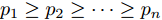
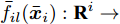
$ \Sigma_i $ 和自适应参数$ \hat{\vartheta}_i $ 的初始值设置为$ [x_1(0),x_2(0)]^{\rm{T}} = [-0.5,0.4]^{\rm{T}} $ ,$ \hat{\vartheta}_i(0) = 0 $ ,$i = 1,2$ . 控制器参数$ k_1 = 2 $ ,$ k_2 = 1 $ ,$ \mu_1 = 4 $ ,$ \mu_2 = 2 $ ,$ \sigma_1 = 3 $ ,$ \sigma_2 = 2 $ ,$ \gamma_1 = 2 $ ,$ \gamma_2 = 3 $ ,$ \delta_1 = \delta_2 = 0.01 $ 和$ \lambda_1 = \lambda_2 = 0.002 $ , 其中,$ \mu_1 = 4>|z_1(0)| = 0.5 $ ,$\mu_2 = 2 > |z_2(0)| = {106}/{315}$ . 系统$ \Sigma_1 $ 和$ \Sigma_2 $ 的仿真结果如图2 ~ 4所示. 图2刻画了输出跟踪误差$ y-y_r $ 的变化情况, 图3给出系统的控制信号$ u $ , 图4描述了自适应参数$ \hat{\vartheta}_1 $ 和$ \hat{\vartheta}_2 $ . 从仿真结果可以看出, 本文所提自适应控制策略既能使系统$ \Sigma_1 $ 和$ \Sigma_2 $ 的输出跟踪误差收敛到原点附近的较小邻域内, 又能确保闭环系统的所有信号有界.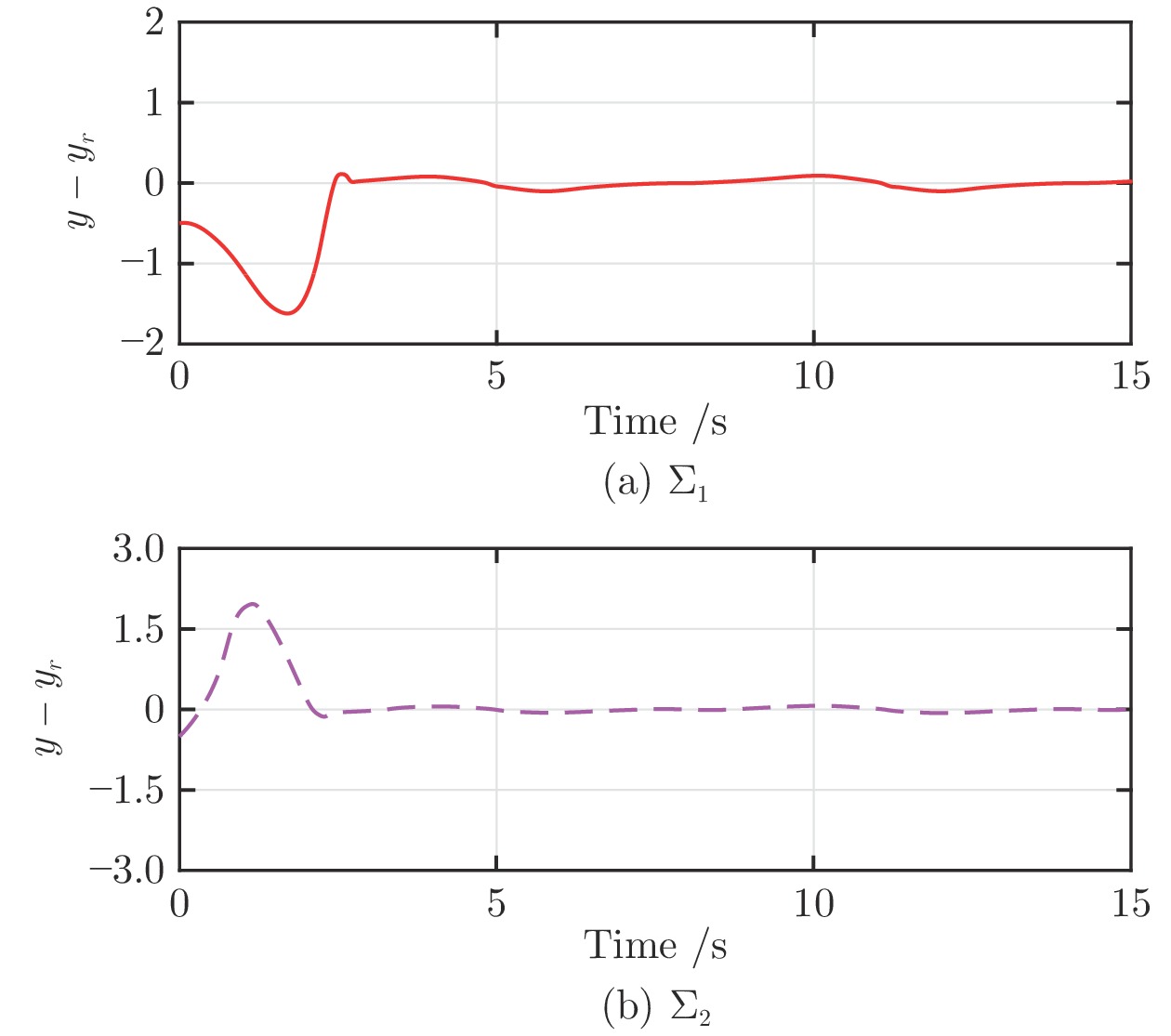 图 2 系统
$\Sigma_1$ 和$\Sigma_2$ 的输出跟踪误差$y-y_r$ Fig. 2 Output tracking errors$y-y_r$ of systems$\Sigma_1$ and$\Sigma_2$ 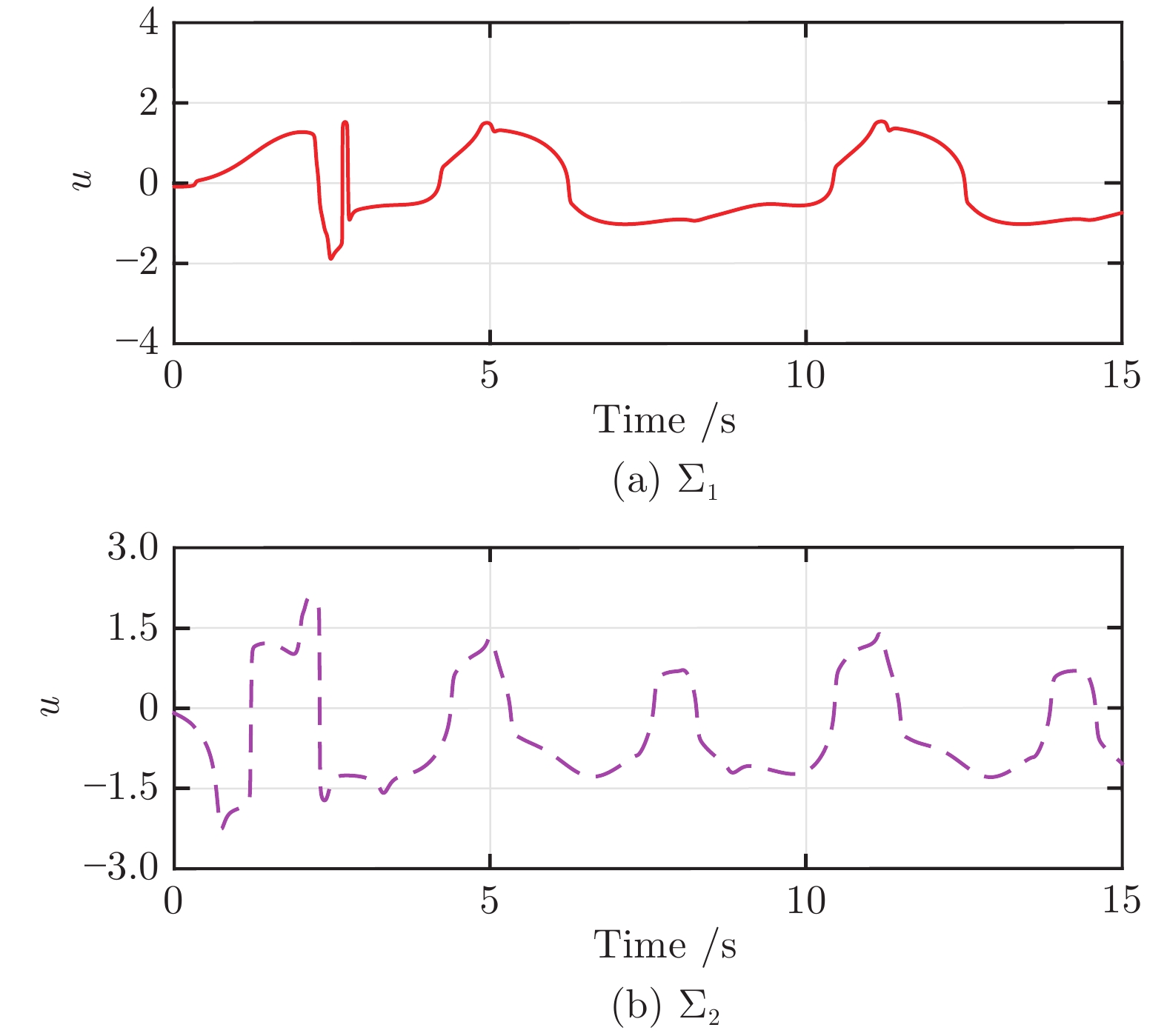 图 3 系统
$\Sigma_1$ 和$\Sigma_2$ 的控制信号$u$ Fig. 3 Control signals$u$ of systems$\Sigma_1$ and$\Sigma_2$  图 4 系统
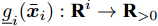
$\Sigma_1$ 和$\Sigma_2$ 的自适应参数$\hat{\vartheta}_1$ 和$\ \hat{\vartheta}_2$ Fig. 4 Adaptive parameters$\hat{\vartheta}_1$ and$\hat{\vartheta}_2$ of systems$\Sigma_1$ and$\Sigma_2$ 为进一步验证本文控制算法的幂次无关特性, 在系统初始值与控制器参数不变的条件下, 对具有不同幂次
$ p_1 $ 和$ p_2 $ 的系统$ \Sigma_1 $ 进行仿真测试. 仿真结果如图5和图6所示. 图5为系统$ \Sigma_1 $ 在不同幂次$ p_1 $ 和$ p_2 $ 条件下的输出跟踪误差$ y-y_r $ , 图6为相应的控制信号$ u $ . 仿真结果表明, 在不同幂次条件下, 该控制器仍然可以保证闭环系统获得良好的控制性能. 图 5 系统
$\Sigma_1$ 在不同幂次下的跟踪误差$y-y_r$ Fig. 5 Output tracking errors$y-y_r$ of system$\Sigma_1$ under various powers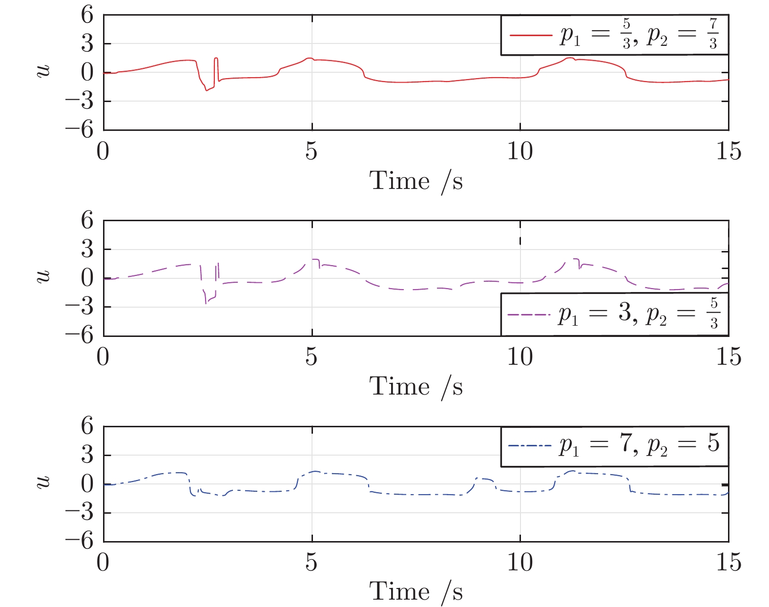 图 6 系统
$\Sigma_1$ 在不同幂次下的控制信号$u$ Fig. 6 Control signals$u$ of system$\Sigma_1$ under various powers4. 结束语
针对一类具有未知幂次的高阶不确定非线性系统, 提出了一种基于障碍李雅普诺夫函数的自适应控制算法. 在无需知晓系统函数先验知识的条件下, 所提控制算法有效克服了系统幂次未知与模型不确定带来的技术挑战. 该算法的显著特点是所设计的自适应控制器均与系统幂次无关. 最后, 仿真结果验证了本文控制算法的有效性与通用性.
今后的研究方向包括将本文所提方法推广到具有未知幂次的高阶非线性系统的输出反馈控制设计[34]. 此外, 为验证本文方法的实用性, 将本文所提控制策略应用于实际系统[35]亦是我们未来研究的目标.
-
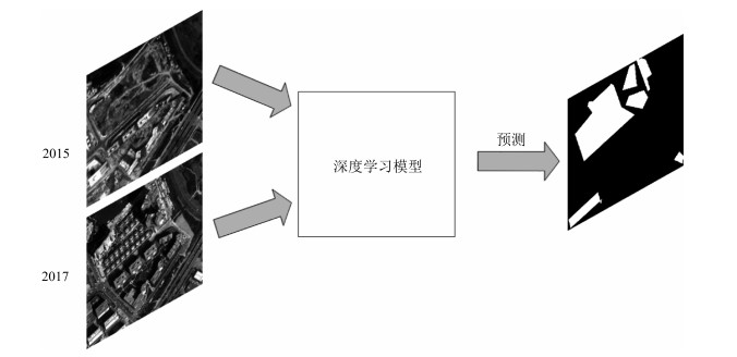
图 1 一种端到端的建筑物变化检测概览图
Fig. 1 An overview of end-to-end architecture of building change detection
图 4 减少拼接区域色差效果图
Fig. 4 The result after the color difference of stitching blocks was sup-pressed

图 10 FlowS-Unet与现有方法的定性比较
Fig. 10 A quality comparison of FlowS-Unet and previous methods
表 1 FlowS-Unet与现有方法的性能比较
Table 1 The performance comparison of FlowS-Unet
序号 方法 F1分数(后处理前/后) 时间(s) 1 FlowS-Unet 0.933/0.943 62 2 FCN 0.858/0.873 50 3 U-Net 0.898/0.913 59 4 人工标注 1.000 18 000  下载: 导出CSV
表 2 多尺度与单尺度训练及预测的F1分数比较
Table 2 The F1 score comparison between multi-scale cross and single-scale training and testing
训练尺度(像素) 预测尺度(像素) F1分数(后处理前/后) 224 224 0.903/0.923 256 256 0.909/0.928 288 288 0.913/0.931 320 320 0.911/0.932 224 0.933/0.939 256 0.938/0.943 多尺度 288 0.939/0.945 320 0.939/0.944 多尺度平均 0.942/0.946
下载: 导出CSV
表 3 FlowS-Unet与其他队伍的F1分数比较
Table 3 The F1 score comparison of FlowS-Unet and other teams
名次 初赛 复赛 决赛 第1名 0.890 0.914 0.861 第2名(FlowS-Unet) 0.903 0.877 0.840 第3名 0.867 0.898 0.800 第4名 0.706 0.870 0.842 第5名 0.879 0.936 0.823
下载: 导出CSV
-
[1] Beumier C, Idrissa M. Building change detection from uniform regions. In: Proceedings of the 17th Iberoamerican Congress Pattern Recognition, Image Analysis, Computer Vision, and Applications. Buenos Aires, Argentina: Springer, 2012. 648-655 [2] Turker M, Sumer E. Building-based damage detection due to earthquake using the watershed segmentation of the post-event aerial images. International Journal of Remote Sensing, 2008, 29(11): 3073-3089 doi: 10.1080/01431160701442096 [3] Huang X, Zhang L P, Zhu T T. Building change detection from multitemporal high-resolution remotely sensed images based on a morphological building index. IEEE Journal of Selected Topics in Applied Earth Observations and Remote Sensing, 2014, 7(1): 105-115 doi: 10.1109/JSTARS.2013.2252423 [4] 周则明, 孟勇, 黄思训, 胡宝鹏.基于能量最小化的星载SAR图像建筑物分割方法.自动化学报, 2016, 42(2): 279-289 doi: 10.16383/j.aas.2016.c150460Zhou Ze-Ming, Meng Yong, Huang Si-Xun, Hu Bao-Peng. Building segmentation of spaceborne SAR images based on energy minimization. Acta Automatica Sinica, 2016, 42(2): 279-289 doi: 10.16383/j.aas.2016.c150460 [5] 李炜明, 吴毅红, 胡占义.视角和光照显著变化时的变化检测方法研究.自动化学报, 2009, 35(5): 449-461 doi: 10.3724/SP.J.1004.2009.00449Li Wei-Ming, Wu Yi-Hong, Hu Zhan-Yi. Urban change detection under large view and illumination variations. Acta Automatica Sinica, 2009, 35(5): 449-461 doi: 10.3724/SP.J.1004.2009.00449 [6] 田昊, 杨剑, 汪彦明, 李国辉.基于先验形状约束水平集模型的建筑物提取方法.自动化学报, 2010, 36(11): 1502-1511 doi: 10.3724/SP.J.1004.2010.01502Tian Hao, Yang Jian, Wang Yan-Ming, Li Guo-Hui. Towards automatic building extraction: Variational level set model using prior shape knowledge. Acta Automatica Sinica, 2010, 36(11): 1502-1511 doi: 10.3724/SP.J.1004.2010.01502 [7] Liu B, Tang K, Liang J. A bottom-up/top-down hybrid algorithm for model-based building detection in single very high resolution SAR image. IEEE Geoscience and Remote Sensing Letters, 2017, 14(6): 926-930 doi: 10.1109/LGRS.2017.2687946 [8] Lukashevich P, Zalessky B, Belotserkovsky A. Building detection on aerial and space images. In: Proceedings of the 2017 International Conference on Information and Digital Technologies (IDT). Zilina, Slovakia: IEEE, 2017. 246-251 [9] 施文灶, 毛政元.基于图分割的高分辨率遥感影像建筑物变化检测研究.地球信息科学学报, 2016, 18(3): 423-432 http://d.old.wanfangdata.com.cn/Periodical/dqxxkx201603017Shi Wen-Zao, Mao Zheng-Yuan. The research on building change detection from high resolution remotely sensed imagery based on graph-cut segmentation. Journal of Geo-Information Science, 2016, 18(3): 423-432 http://d.old.wanfangdata.com.cn/Periodical/dqxxkx201603017 [10] Krizhevsky A, Sutskever I, Hinton G E. ImageNet classification with deep convolutional neural networks. In: Proceedings of the 25th International Conference on Neural Information Processing Systems. Nevada, USA: Curran Associates Inc., 2012. 1097-1105 [11] Simonyan K, Zisserman A. Very deep convolutional networks for large-scale image recognition. In: Proceedings of the 3rd International Conference on Learning Representations. San Diego, California, USA, 2015. 1-14 %arXiv: 1409.1556, 2014. [12] Long J, Shelhamer E, Darrell T. Fully convolutional networks for semantic segmentation. In: Proceedings of the 2015 IEEE Conference on Computer Vision and Pattern Recognition (CVPR). Boston, MA, USA: IEEE, 2015. 3431 -3440 [13] Yuan J Y. Automatic building extraction in aerial scenes using convolutional networks. arXiv: 1602.06564, 2016. [14] Ronneberger O, Fischer P, Brox T. U-Net: Convolutional networks for biomedical image segmentation. In: Proceedings of the 18th Medical Image Computing and Computer-Assisted Intervention. Munich, Germany: Springer, 2015. 234-241 [15] Hariharan B, Arbeláez B, Girshick R, Malik J. Hypercolumns for object segmentation and fine-grained localization. In: Proceedings of the 2015 IEEE Conference on Computer Vision and Pattern Recognition (CVPR). Boston, MA, USA: IEEE, 2015. 447-456 [16] Dosovitskiy A, Fischer P, Ilg E, Häusser P, Hazirbas C, Golkov V, et al. FlowNet: Learning optical flow with convolutional networks. In: Proceedings of the 2015 IEEE International Conference on Computer Vision (ICCV). Santiago, Chile: IEEE, 2015. 2758-2766 [17] 陈文康.基于深度学习的农村建筑物遥感影像检测.测绘, 2016, 39(5): 227-230 doi: 10.3969/j.issn.1674-5019.2016.05.010Chen Wen-Kang. Remote sensing image detection of rural buildings based on deep learning algorithm. Surveying and Mapping, 2016, 39(5): 227-230 doi: 10.3969/j.issn.1674-5019.2016.05.010 [18] Silberman N, Sontag D, Fergus R. Instance segmentation of indoor scenes using a coverage loss. In: Proceedings of the 13th European Conference on Computer Vision. Zurich, Switzerland: Springer, 2014. 616-631 [19] Farabet C, Couprie C, Najman L, LeCun Y. Learning hierarchical features for scene labeling. IEEE Transactions on Pattern Analysis and Machine Intelligence, 2013, 35(8): 1915- 1929 doi: 10.1109/TPAMI.2012.231 [20] Zhang A, Liu X M, Gros A, Tiecke T. Building detection from satellite images on a global scale. arXiv: 1707.08952, 2017. [21] Ghaffarian S, Ghaffarian S. Automatic building detection based on supervised classification using high resolution Google earth images. In: Proceedings of the 2014 ISPRS Technical Commission Ⅲ Symposium. Zurich, Switzerland: ISPRS, 2014. 101-106 [22] Shu Z, Hu X Y, Sun J. Center-point-guided proposal generation for detection of small and dense buildings in aerial imagery. IEEE Geoscience and Remote Sensing Letters, 2018, 15(7): 1100-1104 doi: 10.1109/LGRS.2018.2822760 [23] Yang H L, Lunga D, Yuan J Y. Toward country scale building detection with convolutional neural network using aerial images. In: Proceedings of the 2017 IEEE International Geoscience and Remote Sensing Symposium (IGARSS). Fort Worth, TX, USA: IEEE, 2017. 870-873 [24] Sun L, Tang Y Q, Zhang L P. Rural building detection in high-resolution imagery based on a two-stage CNN model. IEEE Geoscience and Remote Sensing Letters, 2017, 14(11): 1998-2002 doi: 10.1109/LGRS.2017.2745900 [25] Vakalopoulou M, Bus N, Karantzalos K, Paragios N. Integrating edge/boundary priors with classification scores for building detection in very high resolution data. In: Proceedings of the 2017 IEEE International Geoscience and Remote Sensing Symposium (IGARSS). Fort Worth, TX, USA: IEEE, 2017. 3309-3312 [26] Canny J. A computational approach to edge detection. IEEE Transactions on Pattern Analysis and Machine Intelligence, 1986, PAMI-8(6): 679-698 doi: 10.1109/TPAMI.1986.4767851 [27] 卫亚星, 王莉雯.遥感图像增强方法分析.测绘与空间地理信息, 2006, 29(2): 4-7 doi: 10.3969/j.issn.1672-5867.2006.02.002Wei Ya-Xing, Wang Li-Wen. Analysis of enhancement methods about satellite images. Geomatics and Spatial Information Technology, 2006, 29(2): 4-7 doi: 10.3969/j.issn.1672-5867.2006.02.002 [28] Cai B L, Xu X M, Jia K, Qing C M, Tao D C. DehazeNet: An end-to-end system for single image haze removal. IEEE Transactions on Image Processing, 2016, 25(11): 5187-5198 doi: 10.1109/TIP.2016.2598681 [29] Glorot X, Bordes A, Bengio Y. Deep sparse rectifier neural networks. Journal of Machine Learning Research, 2011, 15: 315-323%In: Proceedings of the 14th International Conference on Artificial Intelligence and Statistics. Fort Lauderdale, USA: JMLR W & CP, 2011. 315-323 http://d.old.wanfangdata.com.cn/Periodical/zdhxb201606009 [30] Ioffe S, Szegedy C. Batch normalization: Accelerating deep network training by reducing internal covariate shift. In: Proceedings of the 32nd International Conference on Machine Learning. Lille, France: JMLR, 2015. 448-456 [31] Zeiler M D, Krishnan D, Taylor G W, Fergus R. Deconvolutional networks. In: Proceedings of the 2010 IEEE Computer Society Conference on Computer Vision and Pattern Recognition. San Francisco, CA, USA: IEEE, 2010. 2528- 2535 [32] Srivastava N, Hinton G, Krizhevsky A, Sutskever I, Salakhutdinov R. Dropout: A simple way to prevent neural networks from overfitting. Journal of Machine Learning Research, 2014, 15(1): 1929-1958 http://d.old.wanfangdata.com.cn/Periodical/kzyjc200606005 [33] Lin T Y, Dollár P, Girshick R, He K M, Hariharan B, Belongie S. Feature pyramid networks for object detection. In: Proceedings of the 2017 IEEE Conference on Computer Vision and Pattern Recognition (CVPR). Honolulu, USA: IEEE, 2017. 936-944 [34] Kingma D P, Ba J. Adam: A method for stochastic optimization. In: Proceedings of the 3rd International Conference on Learning Representations. San Diego, CA, USA: 2015. 1-15 期刊类型引用(9)
1. 尹宏伟,杭雨晴,胡文军. 融合异常检测与区域分割的高效K-means聚类算法. 郑州大学学报(工学版). 2024(03): 80-88 .  百度学术
百度学术2. 黄鹤,黄佳慧,刘国权,王会峰,高涛. 采用混合策略联合优化的模糊C-均值聚类信息熵点云简化算法. 西安交通大学学报. 2024(07): 214-226 . 百度学术3. 高瑞贞,王诗浩,王皓乾,张京军,李志杰. 基于图注意力机制的三维点云感知. 中国测试. 2024(07): 155-162 . 百度学术4. 邢建平,殷煜昊. 基于三维重建外点剔除的船舶航迹自适应修正. 舰船科学技术. 2024(14): 162-165 . 百度学术5. 梁循,李志莹,蒋洪迅. 基于图的点云研究综述. 计算机研究与发展. 2024(11): 2870-2896 . 百度学术6. 黄鹤,温夏露,杨澜,王会峰,高涛,茹锋. 基于疯狂捕猎秃鹰算法的K均值互补迭代聚类优化. 浙江大学学报(工学版). 2023(11): 2147-2159 . 百度学术7. 胡建平,刘凯,郭新宇,吴升,温维亮. 自适应加权算子结合主曲线提取玉米叶片点云骨架. 农业工程学报. 2022(02): 166-174 . 百度学术8. 任彪,陆玲. 基于PCL三维点云花瓣分割与重建. 现代电子技术. 2022(12): 149-154 . 百度学术9. 吴艳娟,王健,王云亮. 基于骨架提取算法的作物茎秆识别与定位方法. 农业机械学报. 2022(11): 334-340 . 百度学术其他类型引用(15)
-


 下载:
下载:


计量
- 文章访问数: 2437
- HTML全文浏览量: 397
- PDF下载量: 322
- 被引次数: 24
