

-
摘要: 针对K2算法过度依赖节点序和节点序搜索算法评价节点序效率较低的问题, 提出一种基于节点块序列约束的局部贝叶斯网络结构搜索算法, 该算法首先通过评分定向构建定向支撑树结构, 在此基础上构建节点块序列, 然后利用节点块序列确定每个节点的潜在父节点集, 通过搜索每个节点的父节点集构建网络结构, 最后对该结构进行非法结构修正得到最优贝叶斯网络结构.利用标准网络将算法与几种不同类型的改进算法进行对比分析, 验证该算法的有效性.Abstract: The performance of the K2 algorithm depends on node ordering heavily. The Bayesian learning algorithm based on node order search needs to evaluate the quality of the node sequence by K2 algorithm, resulting in the problem of low efficiency in large and medium-sized networks. In this paper, a new Bayesian structure learning algorithm is proposed to solve the BN structure learning problem by searching local Bayesian network structure construction using node chunk sequence constraints. The algorithm firstly constructs a directional maximum weight spanning tree structure by using score orientation and generates the node chunk sequence by this structure. Then, the node chunk sequence is used to determine the potential parent node set of each node. The network structure is built by searching the parent node set of each node, and the structure is modified by illegal structure to get the optimal Bayesian network structure. Finally, some experiments are designed to evaluate the performance of the proposed algorithm, in which the standard network is used to compare the algorithm with several different improved algorithms to verify the effectiveness of the algorithm. The results indicate that the proposed algorithm is worthy of being studied in the field of BNs construction.
-
Key words:
- Bayesian network structure learning /
- directional maximum weight spanning tree /
- the node chunk sequence /
- K2 algorithm
-
在工业生产和社会生活中, 存在着大量的复杂系统, 如非线性耦合机械系统[1]、超临界机组[2]等. 这些复杂系统线性化时通常包含了不可控模态, 给其控制器设计与分析带来了挑战. 在过去十几年里, 这类称之为高阶非线性系统的自适应控制问题吸引了很多研究者的关注. Lin等在文献[3-4]中提出了一种新的构造性设计框架−增加幂次积分法, 有效解决了高阶非线性系统的镇定与实际跟踪问题. 借助于这一方法, 文献[5-19]研究了不同条件下高阶不确定非线性系统的自适应控制问题, 取得了一系列研究成果. 值得指出的是, 上述绝大多数研究结果都要求系统的幂次信息完全已知. 然而, 在一些实际应用中, 由于控制系统本身与周围环境存在着各种不确定因素, 使得系统的幂次信息可能无法精确获取. 因此, 进一步探讨具有未知幂次的高阶非线性系统的控制器设计是很有意义并值得研究的问题.
针对具有未知幂次的高阶非线性系统, 文献[20-21]采用改进的增加幂次积分法, 分别给出了状态反馈和输出反馈控制算法. 然而, 这些算法没有考虑系统函数的不确定性, 且需要假设系统的幂次上界信息已知. 文献[22]结合增加幂次积分技术和自适应控制方法, 解决了具有未知幂次和不确定参数的高阶非线性系统的自适应控制问题. 最近, 针对一类具有未知时变幂次的高阶非线性系统, 文献[23]利用障碍李雅普诺夫方法给出了满足全状态约束条件的自适应控制方案. 但文献[22-23]所提控制方案仍然要求系统幂次的上界已知. 为去除这一假设条件, 文献[24]采用增加幂次积分技术和逻辑切换方法, 设计了一种全局切换自适应镇定方案. 该方案的不足在于切换控制信号是非光滑的, 可能会引起抖振问题, 从而激发系统中的高频未建模动态. 为此, 文献[25]利用动态增益法, 提出了一种光滑自适应状态反馈控制器, 但这种控制器仅适用于相对阶为2的非线性系统.
基于以上讨论, 本文研究了一类具有未知幂次的高阶不确定非线性系统的自适应跟踪控制问题. 结合积分反推技术和障碍李雅普诺夫函数, 提出了一种新颖的自适应状态反馈控制策略. 本文所得到的控制策略具有如下优点: 1) 采用对数型障碍李雅普诺夫函数[26-27]解决了系统幂次未知与模型不确定带来的技术难题; 2) 所提出的自适应控制策略中没有包含虚拟控制律的导数信息, 避免了积分反推法中的“计算膨胀”问题; 3) 所设计控制器能够确保闭环系统的所有信号一致有界. 最后, 仿真结果验证了本文理论结果的有效性.
本文采用如下符号:
$ {\bf{R}} $ ,${\bf{R}}_{\geq{{0}}}$ ,${\bf{R}}_{ > {{0}}}$ 分别表示实数、非负实数和正实数集合.$ {{\bf{R}}}^n $ 表示$ n $ 维实向量集合.$ {\rm{sign}}(s) $ 表示变量$ s $ 的符号函数. 对任意正常数$ q $ , 定义$ [s]^q = {\rm{sign}}(s)|s|^q $ .${\bf{Q}}_{{\rm{odd}}}^{\ge 1}$ 表示分子和分母都是正奇整数的所有有理数的集合.1. 问题描述与预备知识
1.1 问题描述
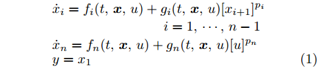
考虑如下高阶不确定非线性系统
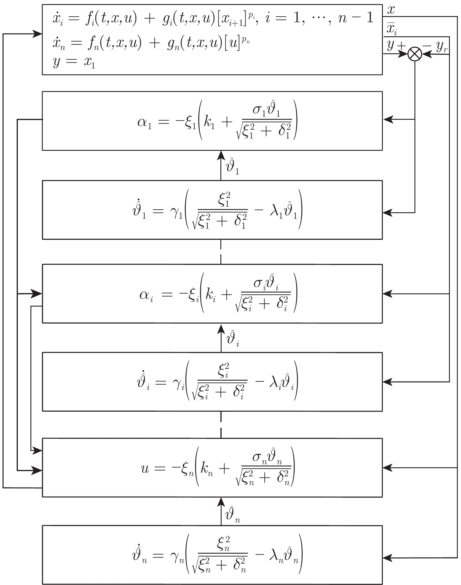
$$ \begin{split} & \dot{x}_i = f_i(t,{\boldsymbol{x}},u)+g_i(t,{\boldsymbol{x}},u)[x_{i+1}]^{p_i}\\ &\qquad\qquad\qquad\;\;\;\;\quad i = 1,\cdots,n-1\\ &\dot{x}_n = f_n(t,{\boldsymbol{x}},u)+g_n(t,{\boldsymbol{x}},u)[u]^{p_n}\\& y = x_1 \end{split} $$ (1) 其中,
${\boldsymbol{x}} = [x_1,\cdots,x_n]^{\rm{T}}\in {{\bf{R}}}^n$ 是系统的状态向量, 初始值${\boldsymbol{x}}(0) = [x_1(0),\cdots,x_n(0)]^{\rm{T}}$ ,$\bar{{\boldsymbol{x}}}_i = [x_1,\cdots,x_i]^{\rm{T}}\in {{\bf{R}}}^i$ ,$i = 1,\cdots,n$ ;$ u \in {{\bf{R}}} $ 和$ y \in {{\bf{R}}} $ 分别是控制输入和系统输出;$ p_i\in {\bf{Q}}_{{\rm{odd}}}^{\ge 1} $ ,$i = 1,\cdots,n$ 是系统(1)的未知幂次. 系统函数$ f_i, g_i:{{\bf{R}}}_{\ge0}\times {{\bf{R}}}^n\times {{\bf{R}}}\rightarrow {{\bf{R}}} $ ,$i = 1,\cdots,n$ 在$ t $ 上分段连续, 且关于$ {\boldsymbol{x}} $ 和$ u $ 满足局部Lipschitz条件. 本文的控制目标是设计自适应控制器$ u $ , 使得系统输出$ y $ 跟踪期望轨迹$ y_r $ , 同时确保闭环系统的所有信号皆有界.注 1. 不同于文献[20-25]中的研究结果, 本文中系统幂次无需满足
$ p_1\ge p_2\ge \cdots\ge p_n $ .假设 1. 存在未知的连续函数
$\bar{f}_{il}(\bar{{\boldsymbol{x}}}_i) : {{\bf{R}}}^{i}\rightarrow {{\bf{R}}}_{\geq0}$ ,$ \underline{g}_i(\bar{{\boldsymbol{x}}}_i): {{\bf{R}}}^{i}\rightarrow {{\bf{R}}}_{>0} $ 和$ \bar{g}_i(\bar{{\boldsymbol{x}}}_i): {{\bf{R}}}^{i}\rightarrow {{\bf{R}}}_{>0} $ , 满足$$ |f_i(t,{\boldsymbol{x}},u)|\le \sum\limits_{l = 1}^{j_i}|x_{i+1}|^{q_{il}}\bar{f}_{il}(\bar{{\boldsymbol{x}}}_i) $$ (2) $$ 0<\underline{g}_i(\bar{{\boldsymbol{x}}}_i)\le g_i(t,{\boldsymbol{x}},u)\le \bar{g}_i(\bar{{\boldsymbol{x}}}_i) $$ (3) 其中,
$i = 1,\cdots,n$ ,$l = 1,\cdots,j_i$ ,$ j_i $ 为有限正整数,$ q_{il} $ 为满足$ 0\le q_{i1}<q_{i2}<\cdots<q_{ij_i}<p_i $ 的正常数.注 2. 假设1表明了本文所提控制算法无需知晓系统函数
$ g_i(t,{\boldsymbol{x}},u) $ ,$ f_i(t,{\boldsymbol{x}},u) $ 及相应的界函数$ \underline{g}_i(\bar{{\boldsymbol{x}}}_{i}) $ ,$ \bar{g}_i(\bar{{\boldsymbol{x}}}_{i}) $ ,$ \bar{f}_{il}(\bar{{\boldsymbol{x}}}_i) $ 的解析表达式.假设 2. 期望轨迹
$ y_r $ 为连续可微函数, 且存在未知正常数$ B_r $ , 满足$$ |y_r(t)|+|\dot{y}_r(t)|\le B_r,t\ge 0 $$ (4) 1.2 预备知识
引理 1[28]. 考虑初值问题
$$ \dot{\boldsymbol{\eta}}_r(t) = h_r(t,{\boldsymbol{\eta}}_r),\; {\boldsymbol{\eta}}_r(0) = {\boldsymbol{\eta}}^0_r\in \Xi_r $$ (5) 其中,
$h_r:{{\bf{R}}}_{\ge0}\times \Xi_r\rightarrow {{\bf{R}}}^{{N}}$ 在$ t $ 上分段连续, 且关于$ {\boldsymbol{\eta}}_r $ 满足局部Lipschitz条件,$\Xi_r\subset {{\bf{R}}}^{{N}}$ 为非空开子集.$ {\boldsymbol{\eta}}_r(t) $ 是初值问题(5)在最大存在区间$ [0,t'_f) $ 上的解,$ t'_f<+\infty $ . 设$ \Xi'_r $ 是$ \Xi_r $ 的紧子集, 则存在$t_s\in [0,t'_f)$ , 使得$ {\boldsymbol{\eta}}_r(t_s)\not\in\Xi'_r $ .引理 2[29]. 对任意
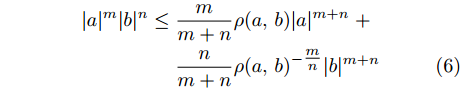
$ a\in {{\bf{R}}} $ ,$ b \in {{\bf{R}}} $ ,$ m\in {{\bf{R}}}_{>0} $ ,$ n\in {{\bf{R}}}_{>0} $ 和函数$ \rho(a,b)>0 $ , 下列不等式成立$$\begin{split} |a|^m|b|^n \le\;& \frac{m}{m+n}\rho(a,b)|a|^{m+n}\;+\\&\frac{n}{m+n}\rho(a,b)^{-\tfrac{m}{n}}|b|^{m+n} \end{split}$$ (6) 引理 3[29-30]. 对任意
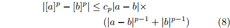
$ p\ge 1 $ ,$ a\in {{\bf{R}}} $ ,$ b \in {{\bf{R}}} $ , 下列不等式成立$$ \|a|^{p}-|b|^{p}|\le |[a]^{p}-[b]^{p}| \hspace{37pt} $$ (7) $$ \begin{split} \,|[a]^{p}-[b]^{p}|\le\; &c_{p}|a-b|\times\\ &(|a-b|^{{p}-1}+|b|^{{p}-1}) \end{split} $$ (8) $$ |a|^{p}+|b|^{p}\le(|a|+|b|)^{p} \hspace{45pt}$$ (9) 其中,
$ c_{p} = 2^{p-2}+2 $ .引理 4[31]. 对任意
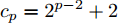
$ \delta\in {{\bf{R}}}_{>0} $ 和$ \xi \in {{\bf{R}}} $ , 下列不等式成立$$ 0\le |\xi|-\frac{\xi^2}{\sqrt{\xi^2+\delta^2}}<\delta $$ (10) 引理 5[32]. 对满足
$ 0\le d<c $ 的$ c\in {{\bf{R}}} $ 和$ d\in {{\bf{R}}} $ , 下列不等式成立$$ \log\frac{c}{c-d} \le \frac{d}{c-d} $$ (11) 2. 自适应跟踪控制策略
本节设计了一种基于障碍李雅普诺夫函数的自适应跟踪控制器, 并给出了闭环系统的稳定性证明.
2.1 自适应控制器设计
定义如下误差坐标变换
$$ z_1 = x_1-y_r $$ (12) $$ z_i = x_i-\alpha_{i-1},\;i = 2,\cdots,n $$ (13) 其中,
$ \alpha_{i-1} $ 是第$ i-1 $ 步的虚拟控制律.步骤
$ {\boldsymbol{i}} $ ${\boldsymbol{(i = 1,\cdots,n-1)}}$ . 选取正常数$ \mu_i $ 满足$ \mu_i>|z_i(0)| $ , 设计第$ i $ 步虚拟控制律和自适应律为$$ \alpha_i = -\xi_i\left(k_i+\frac{\sigma_i\hat{\vartheta}_i}{\sqrt{\xi_i^2+\delta_i^2}}\right) $$ (14) $$ \dot{\hat{\vartheta}}_i = \gamma_i\left(\frac{\xi_i^2}{\sqrt{\xi_i^2+\delta_i^2}}-\lambda_i\hat{\vartheta}_i\right) $$ (15) 其中,
$\xi_i = \dfrac{z_i}{\mu_i^2-z_i^{2}}$ ,$ \hat{\vartheta}_i $ 是$ \vartheta_i $ 的估计值,$ \hat{\vartheta}_i(0)\ge 0 $ ,$ k_i $ ,$ \sigma_i $ ,$ \gamma_i $ 和$ \lambda_i $ 为正常数.步骤 n. 选取正常数
$ \mu_n $ 满足$ \mu_n>|z_n(0)| $ , 设计实际控制律和自适应律为$$ u = -\xi_n\left(k_n+\frac{\sigma_n\hat{\vartheta}_n}{\sqrt{\xi_n^2+\delta_n^2}}\right) $$ (16) $$ \dot{\hat{\vartheta}}_n = \gamma_n\left(\frac{\xi_n^2}{\sqrt{\xi_n^2+\delta_n^2}}-\lambda_n\hat{\vartheta}_n\right) $$ (17) 其中,
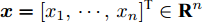
$\xi_n = \dfrac{z_n}{\mu_n^2-z_n^{2}}$ ,$ \hat{\vartheta}_n $ 是$ \vartheta_n $ 的估计值且满足,$\hat{\vartheta}_n(0)\ge 0$ ,$ k_n $ ,$ \sigma_n $ ,$ \gamma_n $ 和$ \lambda_n $ 为正常数.上述自适应控制器的设计过程如图1所示.
注 3. 如式(14) ~ (17)所示, 本文提出的自适应反推控制策略不依赖于系统幂次
$ p_i $ 及其上界信息, 且无需知晓系统函数$ f_i(t,{\boldsymbol{x}},u) $ ,$ g_i(t,{\boldsymbol{x}},u) $ 及相应的界函数$ \bar{f}_{il}(\bar{{\boldsymbol{x}}}_i) $ ,$ \underline{g}_i(\bar{{\boldsymbol{x}}}_{i}) $ ,$ \bar{g}_i(\bar{{\boldsymbol{x}}}_{i}) $ 的解析表达式. 同时, 该控制策略未包含虚拟控制律$ \alpha_i $ 的导数, 消除了积分反推法中“计算膨胀”问题.2.2 稳定性分析
在给出闭环系统的稳定性分析之前, 先引入如下命题.
命题 1. 对式(14) ~ (17)的
$\hat{\vartheta}_1,\cdots,\hat{\vartheta}_n, \alpha_1,\cdots, \alpha_{n-1}$ 和$ u $ , 下列陈述成立i)
$ \hat{\vartheta}_i(t)\ge 0 $ ,$i = 1,\cdots,n$ .ii)
$\xi_i[\alpha_i]^{p_i} = -|\xi_i||\alpha_i|^{p_i} \le 0, \xi_n [u]^{p_n} = -|\xi_n| |u|^{p_n}$ ,$i = 1,\cdots,n-1$ .证明. i) 由于
$\dfrac{\xi_i^2}{\sqrt{\xi_i^2+\delta_i^2}}\ge 0$ 和$ \hat{\vartheta}_i(0)\ge 0 $ , 根据式(15)和式(17), 可直接推出$ \hat{\vartheta}_i(t)\ge 0 $ ,$i = 1,\cdots,n$ .ii) 根据式(14)和式(16),
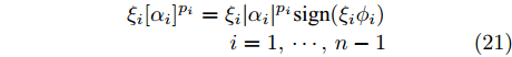
$ \alpha_i $ ,$i = 1,\cdots,n-1$ 和$ u $ 改写为$$ \alpha_i = \xi_i\phi_i,i = 1,\cdots,n-1 $$ (18) $$ u = \xi_n\phi_n\hspace{74pt} $$ (19) 其中,
$$ \phi_i = -k_i-\frac{\sigma_i\hat{\vartheta}_i}{\sqrt{\xi_i^2+\delta_i^2}},\;\;i = 1,\cdots,n $$ (20) 从而, 有
$$ \begin{split} \xi_i[\alpha_i]^{p_i} =&\; \xi_i|\alpha_i|^{p_i}{\rm{sign}}(\xi_i\phi_i)\\& \quad i = 1,\cdots,n-1\end{split} $$ (21) $$ \xi_n [u]^{p_n} = \xi_n |u|^{p_n}{\rm{sign}}(\xi_n\phi_n) $$ (22) 另外, 由于
$ \hat{\vartheta}_i(t)\ge 0 $ ,$i = 1,\cdots,n$ , 从式(20)易知$ \phi_i\le 0 $ ,$i = 1,\cdots,n$ , 进而可得${\rm{sign}}(\xi_i\phi_i) = -{\rm{sign}}(\xi_i)$ ,$i = 1,\cdots,n$ . 故$$ \begin{split} \xi_i[\alpha_i]^{p_i} =&\; -|\xi_i||\alpha_i|^{p_i}\le 0\\ & i = 1,\cdots,n-1 \end{split}$$ (23) $$ \xi_n [u]^{p_n} = -|\xi_n| |u|^{p_n}\le 0 $$ (24) □
本文主要结论可总结为如下定理.
定理 1. 对满足假设1和假设2的高阶不确定非线性系统(1), 在任意初始条件
$ {\boldsymbol{x}}(0) $ 下, 控制器(16)以及自适应律(15)和(17)保证了闭环系统的所有信号一致有界, 并且输出跟踪误差可以收敛到残差为任意小的残差集.证明. 本证明共分为3部分. 首先, 证明由系统(1), 控制器(16), 自适应律(15)和(17)组成的闭环系统在最大存在区间
$ [0,t_f) $ 上存在唯一解${\pmb\eta}(t) = [z_1(t),\cdots,z_n(t),\hat{\vartheta}_1(t),\cdots,\hat{\vartheta}_n(t)]^{\rm{T}}$ . 然后, 采用反证法证明$ t_f = +\infty $ . 最后, 实现本文控制目标.Part 1. 根据式(14)和式(16), 虚拟控制律
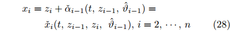
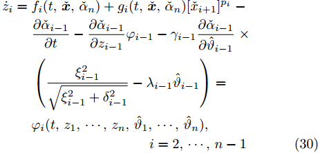
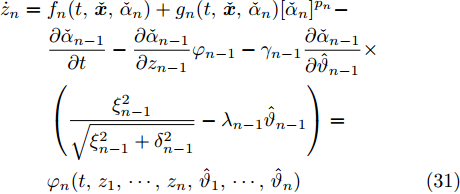
$\alpha_1,\cdots, \alpha_{n-1}$ , 实际控制律$ u $ 以及系统状态$x_1,\cdots,x_n$ 可写为$$ \alpha_i = \check{\alpha}_i(z_i,\hat{\vartheta}_i),i = 1,\cdots,n-1 $$ (25) $$ u = \check{\alpha}_n(z_n,\hat{\vartheta}_n) $$ (26) $$ x_1 = z_1+y_r= \check{x}_1(t,z_1) $$ (27) $$ \begin{split} x_i =\; & z_i+\check{\alpha}_{i-1}(t,z_{i-1},\hat{\vartheta}_{i-1})=\\ & \check{x}_i(t,z_{i-1},z_i,\;\hat{\vartheta}_{i-1}),i = 2,\cdots,n \end{split} $$ (28) 因此, 由式(1)和式(14)
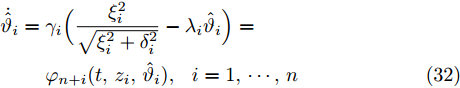
$ \sim $ (17)组成的闭环系统可改写为$$ \begin{split} \dot{z}_1 =\;& f_1(t,\check{{\boldsymbol{x}}},\check{\alpha}_n)+g_1(t,\check{{\boldsymbol{x}}},\check{\alpha}_n)[\check{x}_2]^{p_1}-\dot{y}_r=\\ &\varphi_1(t,z_1,\cdots,z_n,\hat{\vartheta}_1,\cdots,\hat{\vartheta}_n) \end{split} $$ (29) $$ \begin{split} \dot{z}_i = \;& f_i(t,\check{{\boldsymbol{x}}},\check{\alpha}_n)+g_i(t,\check{{\boldsymbol{x}}},\check{\alpha}_n)[\check{x}_{i+1}]^{p_i}\;-\\ &\frac{\partial \check{\alpha}_{i-1}}{\partial t}-\frac{\partial \check{\alpha}_{i-1}}{\partial z_{i-1}}\varphi_{i-1}-\gamma_{i-1}\frac{\partial \check{\alpha}_{i-1}}{\partial \hat{\vartheta}_{i-1}}\;\times\\ &\left(\frac{\xi_{i-1}^2}{\sqrt{\xi_{i-1}^2+\delta_{i-1}^2}}-\lambda_{i-1}\hat{\vartheta}_{i-1}\right)=\\ & \varphi_i(t,z_1,\cdots,z_n,\hat{\vartheta}_1,\cdots,\hat{\vartheta}_n),\\ &\qquad\qquad\qquad\qquad\;\; i = 2,\cdots,n-1 \end{split}$$ (30) $$ \begin{split} \dot{z}_n =\; &f_n(t,\check{{\boldsymbol{x}}},\check{\alpha}_n)+g_n(t,\check{{\boldsymbol{x}}},\check{\alpha}_n)[\check{\alpha}_n]^{p_n}-\\ &\frac{\partial \check{\alpha}_{n-1}}{\partial t}-\frac{\partial \check{\alpha}_{n-1}}{\partial z_{n-1}}\varphi_{n-1}-\gamma_{n-1}\frac{\partial \check{\alpha}_{n-1}}{\partial \hat{\vartheta}_{n-1}}\times\\ &\left(\frac{\xi_{n-1}^2}{\sqrt{\xi_{n-1}^2+\delta_{n-1}^2}}-\lambda_{n-1}\hat{\vartheta}_{n-1}\right)=\\& \varphi_n(t,z_1,\cdots,z_n,\hat{\vartheta}_1,\cdots,\hat{\vartheta}_n) \end{split}$$ (31) $$ \begin{split} \dot{\hat{\vartheta}}_i =\;& \gamma_i\Big(\frac{\xi_i^2}{\sqrt{\xi_i^2+\delta_i^2}}-\lambda_i\hat{\vartheta}_i\Big)=\\ & \varphi_{n+i}(t,z_i,\hat{\vartheta}_i),\;\;i = 1,\cdots,n \end{split} $$ (32) 其中,
$\check{{\boldsymbol{x}}} = [\check{x}_1,\cdots,\check{x}_n]^{\rm{T}}\in {{\bf{R}}}^n$ .定义开集
$$ \Xi = \underbrace{(-\mu_1,\mu_1)\times\cdots\times(-\mu_n,\mu_n)}_n\times {{\bf{R}}}^n $$ 由于
$\mu_i > |z_i(0)|$ ,$i = 1,\cdots,n$ , 可知${\boldsymbol{\eta}}(0) = [z_1(0), \cdots, z_n(0),\hat{\vartheta}_1(0),\cdots,\hat{\vartheta}_n(0)]^{\rm{T}}\in \Xi$ . 同时, 由于期望参考信号$ y_r $ 及其导数$ \dot{y}_r $ 有界, 函数$ f_i, g_i $ ,$i = 1,\cdots, n$ 在$ t $ 上分段连续, 且关于$ {\boldsymbol{x}} $ 和$ u $ 满足局部Lipschitz条件, 可推得$ \varphi_i:{{\bf{R}}}_{\ge0}\times \Xi\rightarrow {{\bf{R}}} $ 在$ t $ 上分段连续, 且关于$ {\boldsymbol{x}} $ 和$ u $ 满足局部Lipschitz条件. 根据微分方程解的存在唯一性定理[33], 对任意初始条件$ {\boldsymbol{\eta}}(0) $ , 闭环系统(29) ~ (32)在最大存在区间$ [0,t_f) $ 上存在唯一解${\boldsymbol{\eta}} = [z_1,\cdots,z_n,\hat{\vartheta}_1,\cdots,\hat{\vartheta}_n]^{\rm{T}}\in \Xi$ , 即, 对$\forall t\in [0,t_f)$ ,$ |z_i|<\mu_i $ ,$i = 1,\cdots,n$ .Part 2. 本部分采用反证法证明
$ t_f = +\infty $ . 为此, 不妨假设$ t_f<+\infty $ .考虑如下障碍李雅普诺夫函数[26]:
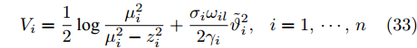
$$ V_i = \frac{1}{{2}}\log\frac{\mu_i^2}{\mu_i^2-z_i^{2}}+\frac{\sigma_i\omega_{il} }{2\gamma_i}\tilde{\vartheta}_i^2,\;\;i = 1,\cdots,n $$ (33) 其中,
$ \tilde{\vartheta}_i = \vartheta_i-\hat{\vartheta}_i $ ,$ \omega_{il} $ 是未知正常数.步骤
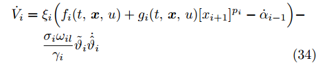
$ {\boldsymbol{i}} $ ${\boldsymbol{(i = 1,\cdots,n-1)}}$ .$ V_i $ 的导数为$$ \begin{split} \dot{V}_i = \;&\xi_i\Big(f_i(t,{\boldsymbol{x}},u)+g_i(t,{\boldsymbol{x}},u)[x_{i+1}]^{p_i}-\dot{\alpha}_{i-1}\Big)-\\ &\frac{\sigma_i\omega_{il} }{\gamma_i}\tilde{\vartheta}_i\dot{\hat{\vartheta}}_i \\[-10pt]\end{split}$$ (34) 其中,
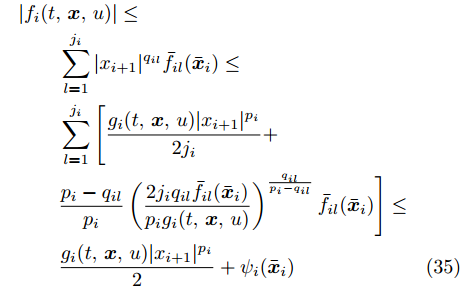
$ \alpha_0 = y_r $ .根据假设1和引理2, 下列不等式成立
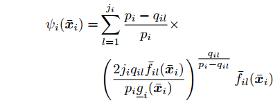
$$ \begin{split} &|f_i(t,{\boldsymbol{x}},u)|\le\\ &\qquad\sum\limits_{l = 1}^{j_i}|x_{i+1}|^{q_{il}}\bar{f}_{il}(\bar{{\boldsymbol{x}}}_i)\le\\ &\qquad\sum\limits_{l = 1}^{j_i}\Bigg[\frac{g_i(t,{\boldsymbol{x}},u)|x_{i+1}|^{p_i}}{2j_i}+\\ &\qquad\frac{p_i-q_{il}}{p_i}\left(\frac{2j_iq_{il}\bar{f}_{il}(\bar{{\boldsymbol{x}}}_i)}{p_ig_i(t,{\boldsymbol{x}},u)}\right)^{\frac{q_{il}}{p_i-q_{il}}}\bar{f}_{il}(\bar{{\boldsymbol{x}}}_i)\Bigg]\le\\ &\qquad\frac{g_i(t,{\boldsymbol{x}},u)|x_{i+1}|^{p_i}}{2}+\psi_i(\bar{{\boldsymbol{x}}}_i) \end{split} $$ (35) 其中,
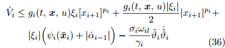
$$ \begin{split} \psi_i(\bar{{\boldsymbol{x}}}_i) =& \sum\limits_{l = 1}^{j_i}\frac{p_i-q_{il}}{p_i}\times\\ &\left(\frac{2j_iq_{il}\bar{f}_{il}(\bar{{\boldsymbol{x}}}_i)}{p_i\underline{g}_i(\bar{{\boldsymbol{x}}}_i)}\right)^{\tfrac{q_{il}}{p_i-q_{il}}}\bar{f}_{il}(\bar{{\boldsymbol{x}}}_i) \end{split}$$ 将式(35)代入式(34), 可得
$$ \begin{split} \dot{V}_i\le\; &g_i(t,{\boldsymbol{x}},u)\xi_i [x_{i+1}]^{p_i}+\frac{g_i(t,{\boldsymbol{x}},u)|\xi_i|}{2}|x_{i+1}|^{p_i}+\\& |\xi_i|\Big(\psi_i(\bar{{\boldsymbol{x}}}_i)+|\dot{\alpha}_{i-1}|\Big)-\frac{\sigma_i\omega_{il} }{\gamma_i}\tilde{\vartheta}_i\dot{\hat{\vartheta}}_i \\[-10pt]\end{split}$$ (36) 根据命题1, 可得
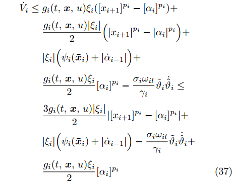
$$ \begin{split} \dot{V}_i\le \;&g_i(t,{\boldsymbol{x}},u)\xi_{i}([x_{i+1}]^{p_i}-[\alpha_{i}]^{p_i})+\\ &\frac{g_i(t,{\boldsymbol{x}},u)|\xi_i|}{2}\Big(|x_{i+1}|^{p_i}-|\alpha_{i}|^{p_i}\Big)+\\ &|\xi_i|\Big(\psi_i(\bar{{\boldsymbol{x}}}_i)+|\dot{\alpha}_{i-1}|\Big)+\\ &\frac{g_i(t,{\boldsymbol{x}},u)\xi_{i}}{2}[\alpha_i]^{p_i}-\frac{\sigma_i\omega_{il} }{\gamma_i}\tilde{\vartheta}_i\dot{\hat{\vartheta}}_i\le\\ &\frac{3g_i(t,{\boldsymbol{x}},u)|\xi_i|}{2}|[x_{i+1}]^{p_i}-[\alpha_{i}]^{p_i}|+\\ &|\xi_i|\Big(\psi_i(\bar{{\boldsymbol{x}}}_i)+|\dot{\alpha}_{i-1}|\Big)-\frac{\sigma_i\omega_{il} }{\gamma_i}\tilde{\vartheta}_i\dot{\hat{\vartheta}}_i+\\& \frac{g_i(t,{\boldsymbol{x}},u)\xi_{i}}{2}[\alpha_i]^{p_i} \end{split}$$ (37) 为了处理式(37)中的项
$ |\xi_i||[x_{i+1}]^{p_i}-[\alpha_{i}]^{p_i}| $ , 考虑以下两种情形.情形 1. 当
$ p_i = 1 $ 时. 由Part 1可得:$|z_{i+1}| < \mu_{i+1}$ ,$ \forall t\in [0,t_f) $ , 因而$$ \begin{split} &|\xi_i||[x_{i+1}]^{p_i}-[\alpha_{i}]^{p_i}|= |\xi_i||z_{i+1}|\le\\ &\qquad \mu_{i+1}|\xi_i|, \;\;\forall t\in [0,t_f) \end{split} $$ (38) 情形 2. 当
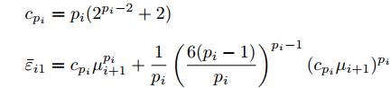
$ p_i>1 $ 时. 由引理2和引理3以及$|z_{i+1}| < \mu_{i+1}$ ,$ \forall t\in [0,t_f) $ , 可得$$\begin{split} &|\xi_i||[x_{i+1}]^{p_i}-[\alpha_{i}]^{p_i}|=\\ &\quad\; \; \; \; |\xi_i||[z_{i+1}+\alpha_{i}]^{p_i}-[\alpha_{i}]^{p_i}|\le\\ &\quad\; \; \; \; c_{p_i}|\xi_i|(\mu_{i+1}^{p_i}+\mu_{i+1}|\alpha_i|^{p_i-1})\le\\ &\quad\; \; \; \; |\xi_i|\Big(\frac{|\alpha_i|^{p_i}}{6}+\bar{\varepsilon}_{i1}\Big),\;\;\forall t\in [0,t_f) \end{split}$$ (39) 其中,
$$ \begin{split} &c_{p_i} = p_i(2^{p_i-2}+2)\\ &\bar{\varepsilon}_{i1} = c_{p_i}\mu_{i+1}^{p_i}+\frac{1}{p_i}\left(\frac{6(p_i-1)}{p_i}\right)^{p_i-1}(c_{p_i}\mu_{i+1})^{p_i} \end{split}$$ 综合情形1和情形2, 项
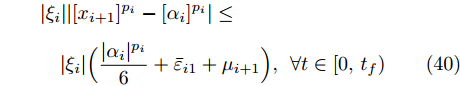
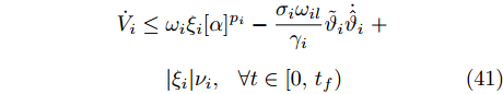
$ |\xi_i||[x_{i+1}]^{p_i}-[\alpha_{i}]^{p_i}| $ 放缩为$$ \begin{split} &|\xi_i||[x_{i+1}]^{p_i}-[\alpha_{i}]^{p_i}| \le\\ &\quad|\xi_i|\Big(\frac{|\alpha_i|^{p_i}}{6}+\bar{\varepsilon}_{i1}+\mu_{i+1}\Big),\;\forall t\in [0,t_f) \end{split} $$ (40) 将式(40)代入式(37)中, 并结合命题1, 易得
$$ \begin{split} \dot{V}_i\le\;&\omega_i\xi_{i}[\alpha]^{p_i}-\frac{\sigma_i\omega_{il} }{\gamma_i}\tilde{\vartheta}_i\dot{\hat{\vartheta}}_i\;+\\ &|\xi_i|\nu_i,\;\;\forall t\in [0,t_f) \end{split} $$ (41) 其中,
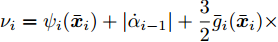
$\omega_i = \dfrac{\underline{g}_i(\bar{{\boldsymbol{x}}}_i)}{4}$ ,$\nu_i = \psi_i(\bar{{\boldsymbol{x}}}_i)+|\dot{\alpha}_{i-1}|+\dfrac{3}{2}\bar{g}_i(\bar{{\boldsymbol{x}}}_{i})\times (\bar{\varepsilon}_{i1}+ \mu_{i+1})$ .由Part 1可知, 对
$ \forall t\in [0,t_f) $ ,$ |z_j|<\mu_j $ ,$j = 1, \cdots, i$ . 同时, 依据假设1和假设2,$ y_r $ ,$ \dot{y}_r $ 有界, 且$ \bar{f}_{il} $ ,$ \underline{g}_i $ 和$ \bar{g}_i $ 为连续函数. 此外, 根据第$ i-1 $ 步设计, 可推知$x_1,\cdots,x_i$ ,$ \dot{\alpha}_{i-1} $ 有界,$ \forall t\in [0,t_f) $ . 因此, 运用极值定理, 对$ \forall t\in [0,t_f) $ , 有$$ 0< \omega_{il}\le \omega_i \, $$ (42) $$ 0\le \nu_i\le \nu_{im} $$ (43) 其中,
$ \omega_{il} $ 和$ \nu_{im} $ 为未知正常数.将式(42)和式(43)代入式(41)中, 有
$$ \begin{split} \dot{V}_i\le\;&\omega_{il}\xi_{i}[\alpha_i]^{p_i}-\frac{\sigma_i\omega_{il} }{\gamma_i}\tilde{\vartheta}_i\dot{\hat{\vartheta}}_i+\\ &\nu_{im}|\xi_i|,\;\;\forall t\in [0,t_f) \end{split} $$ (44) 通过式(14)和式(15), 并结合引理3, 可得
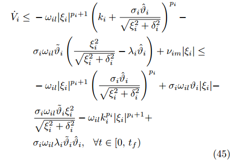
$$ \begin{split} \dot{V}_i\le\;&-\omega_{il}|\xi_{i}|^{p_i+1}\left(k_i+\frac{\sigma_i\hat{\vartheta}_i}{\sqrt{\xi_i^2+\delta_i^2}}\right)^{p_i}-\\& \sigma_i\omega_{il} \tilde{\vartheta}_i\left(\frac{\xi_i^2}{\sqrt{\xi_i^2+\delta_i^2}}-\lambda_i\hat{\vartheta}_i\right)+\nu_{im}|\xi_i|\le\\ &-\omega_{il} |\xi_{i}|^{p_i+1}\left(\frac{\sigma_i\hat{\vartheta}_i}{\sqrt{\xi_i^2+\delta_i^2}}\right)^{p_i}+\sigma_i\omega_{il} \vartheta_i|\xi_i|-\\ &\frac{\sigma_i\omega_{il} \tilde{\vartheta}_i\xi_i^2}{\sqrt{\xi_i^2+\delta_i^2}}-\omega_{il} k_i^{p_i}|\xi_{i}|^{p_i+1}+\\ &\sigma_i\omega_{il} \lambda_i\tilde{\vartheta}_i\hat{\vartheta}_i,\;\;\forall t\in [0,t_f) \end{split} $$ (45) 其中,
$\vartheta_i = \dfrac{\nu_{im}}{\sigma_i\omega_{il}}$ .根据引理2和引理4, 式(45)中的项
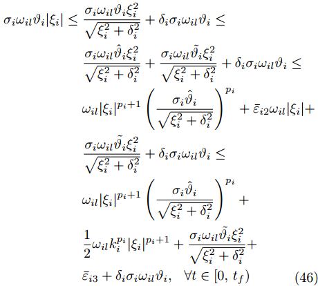
$ \sigma_i\omega_{il}\vartheta_i|\xi_i| $ 放缩为$$ \begin{split} \sigma_i\omega_{il} \vartheta_i|\xi_i|\le\;&\frac{\sigma_i\omega_{il} \vartheta_i\xi_i^2}{\sqrt{\xi_i^2+\delta_i^2}}+\delta_i\sigma_i\omega_{il} \vartheta_i\le\\ &\frac{\sigma_i\omega_{il} \hat{\vartheta}_i\xi_i^2}{\sqrt{\xi_i^2+\delta_i^2}}+\frac{\sigma_i\omega_{il} \tilde{\vartheta_i}\xi_i^2}{\sqrt{\xi_i^2+\delta_i^2}}+\delta_i\sigma_i\omega_{il} \vartheta_i\le\\& \omega_{il} |\xi_{i}|^{p_i+1}\left(\frac{\sigma_i\hat{\vartheta}_i}{\sqrt{\xi_i^2+\delta_i^2}}\right)^{p_i}+\bar{\varepsilon}_{i2}\omega_{il} |\xi_i|+\\ &\frac{\sigma_i\omega_{il} \tilde{\vartheta_i}\xi_i^2}{\sqrt{\xi_i^2+\delta_i^2}}+\delta_i\sigma_i\omega_{il} \vartheta_i\le\\ & \omega_{il} |\xi_{i}|^{p_i+1}\left(\frac{\sigma_i\hat{\vartheta}_i}{\sqrt{\xi_i^2+\delta_i^2}}\right)^{p_i}+\\ &\frac{1}{2}\omega_{il} k_i^{p_i}|\xi_{i}|^{p_i+1}+\frac{\sigma_i\omega_{il} \tilde{\vartheta_i}\xi_i^2}{\sqrt{\xi_i^2+\delta_i^2}}+\\ &\bar{\varepsilon}_{i3}+\delta_i\sigma_i\omega_{il} \vartheta_i,\;\;\forall t\in [0,t_f) \\[-10pt]\end{split} $$ (46) 其中,
$$ \begin{split} &{{\bar \varepsilon }_{i2}} = \left\{ {\begin{array}{*{20}{l}} {0,}&{{p_i} = 1}\\ {\dfrac{{{p_i} - 1}}{{{p_i}}}{{\left(\dfrac{1}{{{p_i}}}\right)}^{\tfrac{1}{{{p_i} - 1}}}},}&{{p_i} > 1} \end{array}} \right.\\ &{{\bar \varepsilon }_{i3}} = \left\{ {\begin{array}{*{20}{l}} {0,}&{{{\bar \varepsilon }_{i2}} = 0}\\ {\dfrac{{{{\bar \varepsilon }_{i2}}{\omega _{il}}{p_i}}}{{{p_i} + 1}}{{\left(\dfrac{{2{{\bar \varepsilon }_{i2}}}}{{k_i^{{p_i}}({p_i} + 1)}}\right)}^{\tfrac{1}{{{p_i}}}}}},&{{{\bar \varepsilon }_{i2}} > 0} \end{array}} \right. \end{split}$$ 由式(45)和式(46), 可得
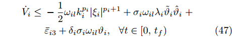
$$\begin{split} \dot{V}_i\le\; &-\frac{1}{2}\omega_{il} k_i^{p_i}|\xi_{i}|^{p_i+1}+\sigma_i\omega_{il} \lambda_i\tilde{\vartheta}_i\hat{\vartheta}_i\;+\\ &\bar{\varepsilon}_{i3}+\delta_i\sigma_i\omega_{il} \vartheta_i,\;\;\forall t\in [0,t_f) \end{split} $$ (47) 依据引理2和引理5, 以及Young不等式, 则有
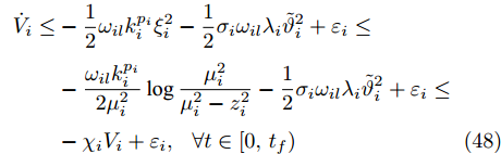
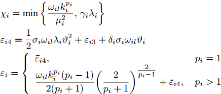
$$ \begin{split} \dot{V}_i\le&-\frac{1}{2}\omega_{il} k_i^{p_i}\xi_{i}^2-\frac{1}{2}\sigma_i\omega_{il} \lambda_i\tilde{\vartheta}_i^2+\varepsilon_i\le\\ &-\frac{\omega_{il} k_i^{p_i}}{2\mu_i^2}\log\frac{\mu_i^2}{\mu_i^2-z_i^{2}}-\frac{1}{2}\sigma_i\omega_{il} \lambda_i\tilde{\vartheta}_i^2+\varepsilon_i\le\\ &-\chi_iV_i+\varepsilon_i,\;\;\forall t\in [0,t_f) \end{split}$$ (48) 其中,
$$ \begin{split} &{\chi _i} = \min \left\{ \frac{{{\omega _{il}}k_i^{{p_i}}}}{{\mu _i^2}},{\gamma _i}{\lambda _i}\right\} \\ &{{\bar \varepsilon }_{i4}} = \frac{1}{2}{\sigma _i}{\omega _{il}}{\lambda _i}\vartheta _i^2 + {{\bar \varepsilon }_{i3}} + {\delta _i}{\sigma _i}{\omega _{il}}{\vartheta _i}\\ &{\varepsilon _i} = \left\{ \begin{array}{*{20}{l}} {{{\bar \varepsilon }_{i4}},}&{{p_i} = 1}\\ {\dfrac{{{\omega _{il}}k_i^{{p_i}}({p_i} - 1)}}{{2({p_i} + 1)}}{{\left(\dfrac{2}{{{p_i} + 1}}\right)}^{\tfrac{2}{{{p_i} - 1}}}} + {{\bar \varepsilon }_{i4}},}&{{p_i} > 1} \end{array} \right. \end{split} $$ 因此, 存在正常数
$ \chi_i^* $ 和$ \varepsilon_i^* $ 满足$$ 0<\chi_i^*\le\chi_i $$ (49) $$ 0<\varepsilon_i\le\varepsilon_i^* $$ (50) 由式(48) ~ (50), 可得
$$ \dot{V}_i\le-\chi_i^*V_i+\varepsilon_i^*,\;\forall t\in [0,t_f) $$ (51) 因此, 对
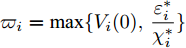
$ \forall t\in [0,t_f) $ 中, 有$$ \frac{1}{2}\log\frac{\mu_i^2}{\mu_i^2-z_i^{2}}\le V_i\le \varpi_i $$ (52) $$ \frac{\sigma_i\omega_{il} }{2\gamma_i}\tilde{\vartheta}_i^2\le V_i\le \varpi_i\;\; \qquad $$ (53) 其中,
$\varpi_i = \max\{V_i(0),\dfrac{\varepsilon_i^*}{\chi_i^*}\}$ .从式(52)和式(53), 可得
$$ |z_i|\le\bar{\mu}_i = \mu_i\sqrt{1-\exp(-{2}\varpi_i)}<\mu_i $$ (54) $$ |\hat{\vartheta}_i|\le\bar{\vartheta}_i = \sqrt{\frac{2\gamma_i\varpi_i}{\sigma_i\omega_{il}}}+\vartheta_i,\;\forall t\in [0,t_f) $$ (55) 进而可推出, 对
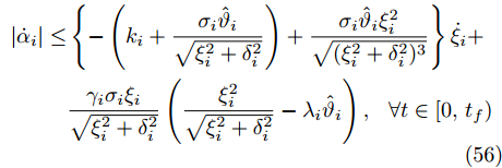
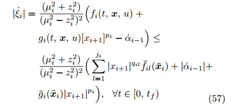
$ \forall t\in [0,t_f) $ ,$ \alpha_i $ 和$ x_{i+1} $ 有界. 接着, 对$ \alpha_i $ 和$ \xi_i $ 分别求导, 可得$$ \begin{split}|\dot{\alpha}_i|\le&\left\{-\left(k_i+\frac{\sigma_i\hat{\vartheta}_i}{\sqrt{\xi_i^2+\delta_i^2}}\right)+\frac{\sigma_i\hat{\vartheta}_i\xi_i^2}{\sqrt{(\xi_i^2+\delta_i^2)^3}}\right\}\dot{\xi}_i+\\ & \frac{\gamma_i\sigma_i\xi_i}{\sqrt{\xi_i^2+\delta_i^2}}\left(\frac{\xi_i^2}{\sqrt{\xi_i^2+\delta_i^2}} -\lambda_i\hat{\vartheta}_i\right),\;\;\forall t\in [0,t_f) \end{split}$$ (56) $$ \begin{split} |\dot{\xi}_i| =\; &\frac{(\mu_i^2+z_i^2)}{(\mu_i^2-z_i^2)^2}\Big(f_i(t,{\boldsymbol{x}},u)\;+\\ &g_i(t,{\boldsymbol{x}},u)[x_{i+1}]^{p_i}-\dot{\alpha}_{i-1}\Big)\le\\ &\frac{(\mu_i^2+z_i^2)}{(\mu_i^2-z_i^2)^2}\Big(\sum\limits_{l = 1}^{j_i}|x_{i+1}|^{q_{il}}\bar{f}_{il}(\bar{{\boldsymbol{x}}}_i)+|\dot{\alpha}_{i-1}|+\\ &\bar{g}_i(\bar{{\boldsymbol{x}}}_{i})|x_{i+1}|^{p_i}\Big),\;\;\forall t\in [0,t_f)\\[-10pt] \end{split} $$ (57) 从式(56)和式(57)可知, 对
$ \forall t\in [0,t_f) $ ,$ \dot{\xi}_i $ 和$ \dot{\alpha}_i $ 亦有界.步骤
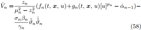
$ {\boldsymbol{n}} $ . 求$ V_n $ 的导数, 可得$$ \begin{split} \dot{V}_n =& \frac{z_n}{\mu_n^2-z_n^{2}}(f_n(t,{\boldsymbol{x}},u) + g_n(t,{\boldsymbol{x}},u)[u]^{p_n}-\dot{\alpha}_{n-1})-\\ &\frac{\sigma_n\beta_n}{\gamma_n}\tilde{\vartheta}_n\dot{\hat{\vartheta}}_n \\[-10pt]\end{split}$$ (58) 类似于式(35)的推导过程, 利用假设1和引理2, 可得
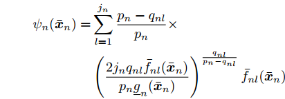
$$ |f_n(t,{\boldsymbol{x}},u)|\le \frac{1}{2}g_n(t,{\boldsymbol{x}},u)|u|^{p_n}+\psi_n(\bar{{\boldsymbol{x}}}_n) $$ (59) 其中,
$$ \begin{split} \psi_n(\bar{{\boldsymbol{x}}}_n) = &\sum\limits_{l = 1}^{j_n}\frac{p_n-q_{nl}}{p_n}\times\\ &\left(\frac{2j_nq_{nl}\bar{f}_{nl}(\bar{{\boldsymbol{x}}}_n)}{p_n\underline{g}_n(\bar{{\boldsymbol{x}}}_n)}\right)^{\frac{q_{nl}}{p_n-q_{nl}}}\bar{f}_{nl}(\bar{{\boldsymbol{x}}}_n) \end{split}$$ 由式(59)以及命题1, 可推得
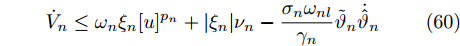
$$ \dot{V}_n\le\omega_n\xi_n[u]^{p_n}+|\xi_n|\nu_n-\frac{\sigma_n\omega_{nl} }{\gamma_n}\tilde{\vartheta}_n\dot{\hat{\vartheta}}_n $$ (60) 其中,
$\omega_n = \dfrac{\underline{g}_n(\bar{{\boldsymbol{x}}}_n)}{2}$ ,$ \nu_n = \psi_n(\bar{{\boldsymbol{x}}}_n)+|\dot{\alpha}_{n-1}| $ .由Part 1可知, 对
$ \forall t\in [0,t_f) $ ,$ |z_j|<\mu_j $ ,$j = 1, \cdots, n$ . 同时, 根据假设1和假设2,$ y_r $ 和$ \dot{y}_r $ 有界, 且$ \bar{f}_{nl} $ ,$ \underline{g}_n $ 和$ \bar{g}_n $ 连续. 此外, 由第$ n-1 $ 步设计可推得$x_1,\cdots, x_n$ ,$ \dot{\alpha}_{n-1} $ 有界,$ \forall t\in [0,t_f) $ . 因此, 运用极值定理, 对$ \forall t\in [0,t_f) $ , 有$$ 0< \omega_{nl}\le \omega_n $$ (61) $$ 0\le \nu_n\le \nu_{nm} $$ (62) 其中,
$ \omega_{nl} $ 和$ \nu_{nm} $ 为未知正常数.利用式(61)和式(62), 有
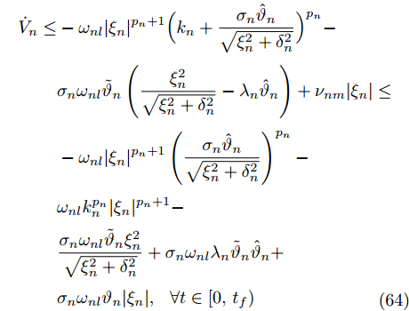
$$ \begin{split} \dot{V}_n\le\;&\omega_{nl}\xi_n[u]^{p_n}+\nu_{nm}|\xi_n|-\\& \frac{\sigma_n\omega_{nl} }{\gamma_n}\tilde{\vartheta}_n\dot{\hat{\vartheta}}_n,\;\;\forall t\in [0,t_f) \end{split} $$ (63) 根据式(16)和式(17)以及命题1和引理3, 可得
$$ \begin{split} \dot{V}_n\le&-\omega_{nl}|\xi_{n}|^{p_n+1}\Big(k_n+\frac{\sigma_n\hat{\vartheta}_n}{\sqrt{\xi_n^2+\delta_n^2}}\Big)^{p_n}-\\ &\sigma_n\omega_{nl} \tilde{\vartheta}_n\left(\frac{\xi_n^2}{\sqrt{\xi_n^2+\delta_n^2}}-\lambda_n\hat{\vartheta}_n\right)+\nu_{nm}|\xi_n|\le\\ & -\omega_{nl} |\xi_{n}|^{p_n+1}\left(\frac{\sigma_n\hat{\vartheta}_n}{\sqrt{\xi_n^2+\delta_n^2}}\right)^{p_n}-\\ &\omega_{nl} k_n^{p_n}|\xi_{n}|^{p_n+1}-\\ &\frac{\sigma_n\omega_{nl} \tilde{\vartheta}_n\xi_n^2}{\sqrt{\xi_n^2+\delta_n^2}}+\sigma_n\omega_{nl} \lambda_n\tilde{\vartheta}_n\hat{\vartheta}_n+\\ &\sigma_n\omega_{nl} \vartheta_n|\xi_n|,\;\;\forall t\in [0,t_f) \\[-10pt]\end{split}$$ (64) 其中,
$\vartheta_n = \dfrac{\nu_{nm}}{\sigma_n\omega_{nl}}$ .依据引理2和引理4, 式(64)中的项
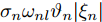
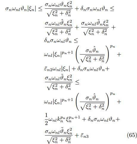
$ \sigma_n\omega_{nl}\vartheta_n|\xi_n| $ 放缩为$$ \begin{split} \sigma_n\omega_{nl} \vartheta_n|\xi_n|\le\;&\frac{\sigma_n\omega_{nl} \vartheta_n\xi_n^2}{\sqrt{\xi_n^2+\delta_n^2}}+\delta_n\sigma_n\omega_{nl} \vartheta_n\le\\ & \frac{\sigma_n\omega_{nl} \hat{\vartheta}_n\xi_n^2}{\sqrt{\xi_n^2+\delta_n^2}}+\frac{\sigma_n\omega_{nl} \tilde{\vartheta}_n\xi_n^2}{\sqrt{\xi_n^2+\delta_n^2}}\;+\\ &\delta_n\sigma_n\omega_{nl} \vartheta_n\le\\ &\omega_{nl} |\xi_n|^{p_n+1}\left(\frac{\sigma_n\hat{\vartheta}_n}{\sqrt{\xi_n^2+\delta_n^2}}\right)^{p_n}+\\ &\bar{\varepsilon}_{n2}\omega_{nl} |\xi_n|+\delta_n\sigma_n\omega_{nl}\vartheta_n+\\ &\frac{\sigma_n\omega_{nl} \tilde{\vartheta}_n\xi_n^2}{\sqrt{\xi_n^2+\delta_n^2}}\le\\ &\omega_{nl} |\xi_n|^{p_n+1}\left(\frac{\sigma_n\hat{\vartheta}_n}{\sqrt{\xi_n^2+\delta_n^2}}\right)^{p_n}+\\ &\frac{1}{2}\omega_{nl} k_n^{p_n}\xi_{n}^{p_n+1}+\delta_n\sigma_n\omega_{nl} \vartheta_n+\\ &\frac{\sigma_n\omega_{nl}\tilde{\vartheta}_n\xi_n^2}{\sqrt{\xi_n^2+\delta_n^2}}+\bar{\varepsilon}_{n3} \end{split} $$ (65) 其中,
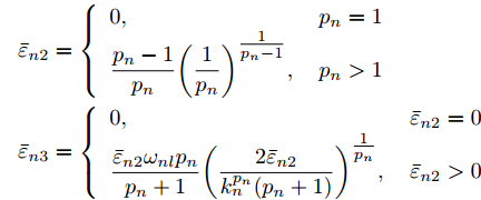
$$ \begin{split} &{{\bar \varepsilon }_{n2}} = \left\{ {\begin{array}{*{20}{l}} {0,}&{{p_n} = 1}\\ {\dfrac{{{p_n} - 1}}{{{p_n}}}{{\left(\dfrac{1}{{{p_n}}}\right)}^{\tfrac{1}{{{p_n} - 1}}}},}&{{p_n} > 1} \end{array}} \right.\\ &{{\bar \varepsilon }_{n3}} = \left\{ {\begin{array}{*{20}{l}} {0,}&{{{\bar \varepsilon }_{n2}} = 0}\\ {\dfrac{{{{\bar \varepsilon }_{n2}}{\omega _{nl}}{p_n}}}{{{p_n} + 1}}{{\left(\dfrac{{2{{\bar \varepsilon }_{n2}}}}{{k_n^{{p_n}}({p_n} + 1)}}\right)}^{\tfrac{1}{{{p_n}}}}},}&{{{\bar \varepsilon }_{n2}} > 0} \end{array}} \right. \end{split} $$ 将式(65)代入式(64)中, 得到
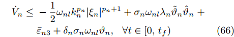
$$ \begin{split} \dot{V}_n\le\;&-\frac{1}{2}\omega_{nl} k_n^{p_n}|\xi_{n}|^{p_n+1}+\sigma_n\omega_{nl} \lambda_n\tilde{\vartheta}_n\hat{\vartheta}_n\;+\\ &\bar{\varepsilon}_{n3}+\delta_n\sigma_n\omega_{nl} \vartheta_n,\;\;\forall t\in [0,t_f) \end{split} $$ (66) 根据引理2和引理5, 以及Young不等式, 可得
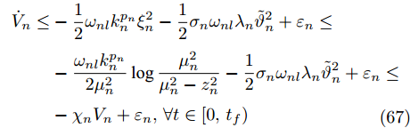
$$ \begin{split} \dot{V}_n\le&-\frac{1}{2}\omega_{nl} k_n^{p_n}\xi_{n}^2-\frac{1}{2}\sigma_n\omega_{nl} \lambda_n\tilde{\vartheta}_n^2+\varepsilon_n\le\\ &-\frac{\omega_{nl} k_n^{p_n}}{2\mu_n^2}\log\frac{\mu_n^2}{\mu_n^2-z_n^{2}}-\frac{1}{2}\sigma_n\omega_{nl} \lambda_n\tilde{\vartheta}_n^2+\varepsilon_n\le\\ &-\chi_nV_n+\varepsilon_n,\forall t\in [0,t_f) \\[-10pt]\end{split} $$ (67) 其中,
$$ \begin{split} &{\chi _n} = \min \left\{ \frac{{{\omega _{nl}}k_n^{{p_n}}}}{{\mu _n^2}},{\gamma _n}{\lambda _n}\right\} \\ &{{\bar \varepsilon }_{n4}} = \frac{1}{2}{\sigma _n}{\omega _{nl}}{\lambda _n}\vartheta _n^2 + {{\bar \varepsilon }_{n3}} + {\delta _n}{\sigma _n}{\omega _{nl}}{\vartheta _n}\\ &{\varepsilon _n} = \left\{ {\begin{array}{*{20}{l}} {{{\bar \varepsilon }_{n4}},}&{{p_n} = 1}\\ {\dfrac{{{\omega _{nl}}k_n^{{p_n}}({p_n} - 1)}}{{2({p_n} + 1)}}{{\left(\dfrac{2}{{{p_n} + 1}}\right)}^{\tfrac{2}{{{p_n} - 1}}}} + {{\bar \varepsilon }_{n4}},}&{{p_n} > 1} \end{array}} \right. \end{split} $$ 因此, 存在正常数
$ \chi_n^* $ 和$ \varepsilon_n^* $ , 使得$$ 0<\chi_n^*\le \chi_n $$ (68) $$ 0<\varepsilon_n\le\varepsilon_n^* \; $$ (69) 根据式(67) ~ (69), 可得
$$ \dot{V}_n\le-\chi_n^*V_n+\varepsilon_n^*,\;\;\forall t\in [0,t_f) $$ (70) 因此, 对
$ \forall t\in [0,t_f) $ , 有$$ \frac{1}{2}\log\frac{\mu_n^2}{\mu_n^2-z_n^{2}}\le V_n\le \varpi_n $$ (71) $$ \frac{\sigma_n\omega_{nl} }{2\gamma_n}\tilde{\vartheta}_n^2\le V_n\le \varpi_n\;\;\;\;\;\;\; $$ (72) 其中,
$\varpi_n = \max\{V_n(0),\dfrac{\varepsilon_n^*}{\chi_n^*}\}$ .由式(71)和式(72), 可得
$$ |z_n|\le \bar{\mu}_n = \mu_n\sqrt{1-\exp(-{2}\varpi_n)}<\mu_n\;\;\;\;\; $$ (73) $$ |\hat{\vartheta}_n|\le\sqrt{\bar{\vartheta}_n = \frac{2\gamma_n\varpi_n}{\sigma_n\omega_{nl}}}+\vartheta_n,\;\; \forall t\in [0,t_f) $$ (74) 故可推出, 对
$ \forall t\in [0,t_f) $ ,$ u $ 有界.由步骤 1 ~
$n $ 可知, 存在紧子集$\Xi' = [-\bar{\mu}_1,\bar{\mu}_1]\,\times \cdots\times [-\bar{\mu}_n, \bar{\mu}_n]\times [-\bar{\vartheta}_1,\bar{\vartheta}_1]\times\cdots\times[-\bar{\vartheta}_n,\bar{\vartheta}_n]\subset \Xi$ , 使得闭环系统在$ [0,t_f) $ 上存在唯一解$ {\boldsymbol{\eta}}(t)\in \Xi' $ . 根据引理1, 可得:$ t_f = +\infty $ , 即, 对$ \forall t \in [0,+\infty) $ ,$|z_i| < \mu_i$ ,$i = 1, \cdots,n$ .Part 3. 重复Part 2中的步骤1 ~ n, 可得
$x_1,\cdots, x_n$ ,$\alpha_1,\cdots,\alpha_{n-1}$ 和$ u $ 均有界,$ \forall t \in [0,+\infty) $ . 另外, 从式(54)可知, 通过减小$ \mu_1 $ 和$ \varpi_1 $ 可将输出跟踪误差$ z_1 $ 收敛到任意小的残差集. □注 4. 不同于文献[20-25]中提出的控制方案, 本文采用积分反推技术和障碍李雅普诺夫方法解决了高阶非线性系统中幂次未知和系统函数不确定的问题, 且所设计控制策略不依赖于未知幂次的上界信息.
3. 仿真算例
为了验证本文所提控制算法的有效性与通用性, 考虑如下两个高阶非线性系统
$$ {\Sigma _1}:\left\{ \begin{aligned} &{{{\dot x}_1} = {f_{1,{\Sigma _1}}} + {g_{1,{\Sigma _1}}}{{[{x_2}]}^{{p_1}}}}\\ &{{{\dot x}_2} = {f_{2,{\Sigma _1}}} + {g_{2,{\Sigma _1}}}{{[u]}^{{p_2}}}}\\ &{y = {x_1}} \end{aligned} \right. $$ (75) $$ {\Sigma _2}:\left\{ \begin{aligned} &{{{\dot x}_1} = {f_{1,{\Sigma _2}}} + {g_{1,{\Sigma _2}}}{{[{x_2}]}^{{p_1}}}}\\ &{{{\dot x}_2} = {f_{2,{\Sigma _2}}} + {g_{2,{\Sigma _2}}}{{[u]}^{{p_2}}}}\\ &{y = {x_1}} \end{aligned} \right. $$ (76) 其中,
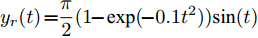
$p_1 = {5}/{3}$ ,$p_2 ={7}/{3}$ ,$ f_{1,\Sigma_1} = x_1\cos (t) $ ,$g_{1,\Sigma_1} = 3+ 0.5\sin (t)$ ,$f_{2,\Sigma_1} = x_1+2\sin (x_1x_2)$ ,$g_{2,\Sigma_1} = 2+ 0.1\sin (t)$ ,$f_{1,\Sigma_2} \;= \;(0.5x_1\; +\; 1)\cos (t)$ ,$g_{1,\Sigma_2} = 2 + 0.1\sin (t)$ ,$f_{2,\Sigma_2} = \cos (x_1 )\exp(2x_2\sin (x_1 )) + x_1x_2\sin (t)$ ,$g_{2,\Sigma_2} = 1$ , 期望参考信号$y_r(t) = \dfrac{\pi}{2}(1 - \exp( -0.1t^2)) \sin (t)$ .在仿真中, 系统
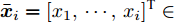
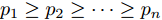
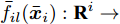
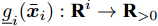
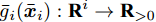
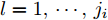
$ \Sigma_i $ 和自适应参数$ \hat{\vartheta}_i $ 的初始值设置为$ [x_1(0),x_2(0)]^{\rm{T}} = [-0.5,0.4]^{\rm{T}} $ ,$ \hat{\vartheta}_i(0) = 0 $ ,$i = 1,2$ . 控制器参数$ k_1 = 2 $ ,$ k_2 = 1 $ ,$ \mu_1 = 4 $ ,$ \mu_2 = 2 $ ,$ \sigma_1 = 3 $ ,$ \sigma_2 = 2 $ ,$ \gamma_1 = 2 $ ,$ \gamma_2 = 3 $ ,$ \delta_1 = \delta_2 = 0.01 $ 和$ \lambda_1 = \lambda_2 = 0.002 $ , 其中,$ \mu_1 = 4>|z_1(0)| = 0.5 $ ,$\mu_2 = 2 > |z_2(0)| = {106}/{315}$ . 系统$ \Sigma_1 $ 和$ \Sigma_2 $ 的仿真结果如图2 ~ 4所示. 图2刻画了输出跟踪误差$ y-y_r $ 的变化情况, 图3给出系统的控制信号$ u $ , 图4描述了自适应参数$ \hat{\vartheta}_1 $ 和$ \hat{\vartheta}_2 $ . 从仿真结果可以看出, 本文所提自适应控制策略既能使系统$ \Sigma_1 $ 和$ \Sigma_2 $ 的输出跟踪误差收敛到原点附近的较小邻域内, 又能确保闭环系统的所有信号有界.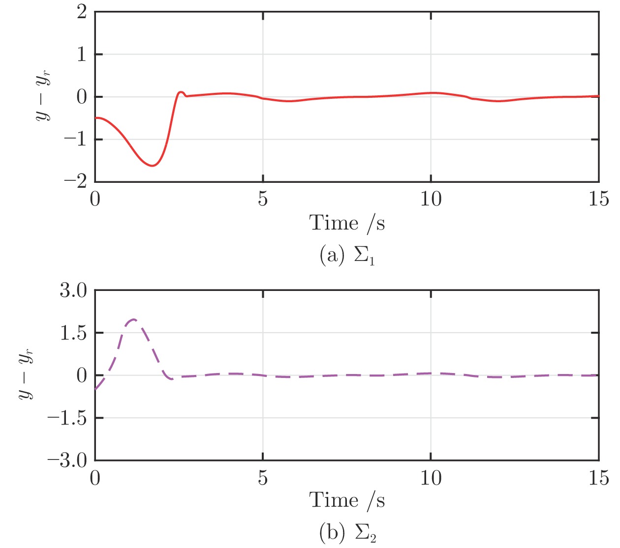 图 2 系统
$\Sigma_1$ 和$\Sigma_2$ 的输出跟踪误差$y-y_r$ Fig. 2 Output tracking errors$y-y_r$ of systems$\Sigma_1$ and$\Sigma_2$ 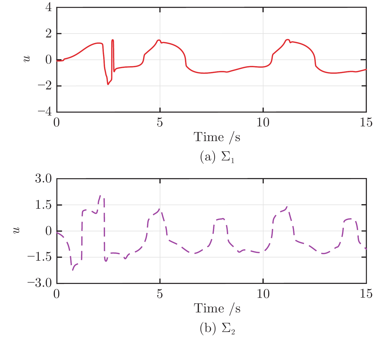 图 3 系统
$\Sigma_1$ 和$\Sigma_2$ 的控制信号$u$ Fig. 3 Control signals$u$ of systems$\Sigma_1$ and$\Sigma_2$  图 4 系统
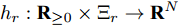
$\Sigma_1$ 和$\Sigma_2$ 的自适应参数$\hat{\vartheta}_1$ 和$\ \hat{\vartheta}_2$ Fig. 4 Adaptive parameters$\hat{\vartheta}_1$ and$\hat{\vartheta}_2$ of systems$\Sigma_1$ and$\Sigma_2$ 为进一步验证本文控制算法的幂次无关特性, 在系统初始值与控制器参数不变的条件下, 对具有不同幂次
$ p_1 $ 和$ p_2 $ 的系统$ \Sigma_1 $ 进行仿真测试. 仿真结果如图5和图6所示. 图5为系统$ \Sigma_1 $ 在不同幂次$ p_1 $ 和$ p_2 $ 条件下的输出跟踪误差$ y-y_r $ , 图6为相应的控制信号$ u $ . 仿真结果表明, 在不同幂次条件下, 该控制器仍然可以保证闭环系统获得良好的控制性能. 图 5 系统
$\Sigma_1$ 在不同幂次下的跟踪误差$y-y_r$ Fig. 5 Output tracking errors$y-y_r$ of system$\Sigma_1$ under various powers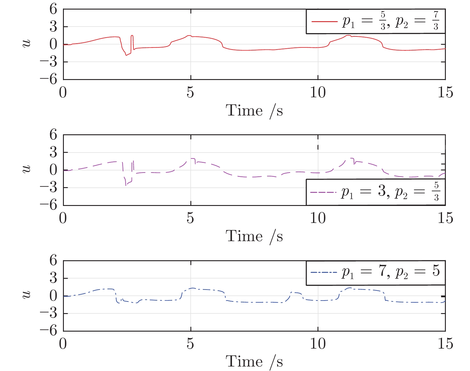 图 6 系统
$\Sigma_1$ 在不同幂次下的控制信号$u$ Fig. 6 Control signals$u$ of system$\Sigma_1$ under various powers4. 结束语
针对一类具有未知幂次的高阶不确定非线性系统, 提出了一种基于障碍李雅普诺夫函数的自适应控制算法. 在无需知晓系统函数先验知识的条件下, 所提控制算法有效克服了系统幂次未知与模型不确定带来的技术挑战. 该算法的显著特点是所设计的自适应控制器均与系统幂次无关. 最后, 仿真结果验证了本文控制算法的有效性与通用性.
今后的研究方向包括将本文所提方法推广到具有未知幂次的高阶非线性系统的输出反馈控制设计[34]. 此外, 为验证本文方法的实用性, 将本文所提控制策略应用于实际系统[35]亦是我们未来研究的目标.
-

图 1 由定向支撑树构建节点块序列的例子
Fig. 1 Example of constructing node chunk sequence by directional support tree

图 2 由节点块序列搜索潜在父节点集的简单例子
Fig. 2 A simple example of searching potential parent set by node chunk sequence
图 3 Alarm网络中不同算法精度对比
Fig. 3 Comparison of different algorithm accuracy in Alarm network
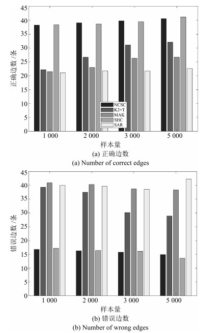
图 4 Insurance网络中不同算法精度对比
Fig. 4 Comparison of different algorithm accuracy in Insurance network
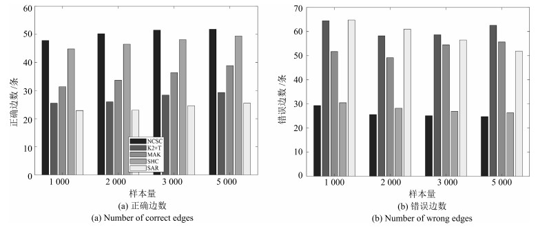
图 5 Hailfinder网络中不同算法精度对比
Fig. 5 Comparison of different algorithm accuracy in Hailfinder network
表 1 标准贝叶斯网络的参数
Table 1 Parameters of standard Bayesian networks
网络 节点数 边数 变量域 最大节点出入度 Alarm 37 46 2~4 6 Insurance 27 52 2~5 9 Hailfinder 56 66 2~11 17  下载: 导出CSV
表 2 标准贝叶斯网络结构平均BIC得分
Table 2 Average BIC score in standard Bayesian network structure
网络 1 000 2 000 3 000 5 000 Alarm -10 874.35 -20 382.51 -30 057.28 -48 056.66 Insurance -15 998.20 -30 103.21 -43 863.15 -73 069.35 Hailfinder -67 046.62 -126 837.31 -176 348.73 -279 766.12
下载: 导出CSV
表 3 NCSC算法与标准节点序的K2算法在Alarm网络中运行结果
Table 3 Results of NCSC algorithm and standard node sequence K2 algorithm in Alarm network
Alarm BIC Ext (s) 结构 C M R A W 1 000 NCSC -11 410.83 32.98±1.82 41.8 2.1 2.8 6.5 11.4 K2 -11 189.51 10.27±0.61 44.2 1.8 0 4.3 6.1 2 000 NCSC -20 791.86 42.14±1.88 41.7 1.9 2.2 6.2 10.3 K2 -20 605.99 11.53±0.47 44.5 1.5 0 2.7 4.2 3 000 NCSC -31 025.28 45.99±5.93 42.9 1.3 2.2 4.2 7.7 K2 -30 505.01 14.04±1.95 44.9 1.1 0 3.1 4.2 5 000 NCSC -49 812.61 56.25±2.13 43.2 1.2 1.1 4.7 7 K2 -49 235.77 16.51±0.74 45.1 1.0 0.0 3.1 4.1
下载: 导出CSV
表 4 NCSC算法与标准节点序的K2算法在Insurance网络中运行结果
Table 4 Results of NCSC algorithm and standard node sequence K2 algorithm in Insurance network
Insurance BIC Ext (s) 结构 C M R A W 1 000 NCSC -16 486.31 17.28±0.34 38.3 11.9 2.3 2.6 16.8 K2 -16 219.71 4.58±0.25 39.7 12.3 0 0.3 12.6 2 000 NCSC -30 756.3 19.61±1.13 39.1 10.7 2.4 3.2 16.3 K2 -30 544.86 5.11±0.31 42.2 9.8 0 0.5 10.3 3 000 NCSC -45 369.23 24.34±3.22 39.8 10.2 2.3 3.3 15.8 K2 -44 748.8 6.32±0.40 42.6 9.4 0 0.5 9.9 5 000 NCSC -73 566.77 29.92±2.91 40.6 9.4 2.3 3.2 14.9 K2 -73 148.28 7.68±0.45 43.8 8.2 0 0.6 8.8
下载: 导出CSV
表 5 NCSC算法与标准节点序的K2算法在Hailfinder网络中运行结果
Table 5 Results of NCSC algorithm and standard node sequence K2 algorithm in Hailfinder network
Insurance BIC Ext (s) 结构 C M R A W 1 000 NCSC -78 396.62 232.18±16.31 47.8 16.3 2.8 9.7 29.3 K2 -78 157.99 25.71±1.55 48.3 17.7 0 8.1 25.8 2 000 NCSC -131 604.2 250.58±7.94 50.2 13.9 1.6 10.1 25.6 K2 -130 945.5 30.22±1.51 51.6 14.4 0 9.1 23.5 3 000 NCSC -182 167.2 292.22±20.01 51.5 13.4 1.4 10.3 25.1 K2 -181 831.9 36.58±1.84 52.9 13.1 0 9.5 22.6 5 000 NCSC -283 288.4 356.14±16.77 51.8 12.8 1.8 10.1 24.7 K2 -282 937.2 43.37±1.83 53.5 12.5 0 9.9 22.4
下载: 导出CSV
表 6 五种算法在Alarm网络中运行时间(s)
Table 6 Running time of five algorithms in Alarm network (s)
Alarm 1 000 2 000 3 000 5 000 NCSC 32.98±1.82 42.14±1.88 45.99±2.04 56.25±2.13 K2+T 11.72±0.74 14.82±1.62 16.33±1.25 18.82±2.71 MAK 942.60±31.4 1 153.37±32.37 1 299.01±42.55 1 582.35±46.86 SHC 3 474.01±90.80 4 079.66±121.98 4 784.10±156.85 6 013.93±216.64 SAR 46.77±0.81 49.64±3.52 62.30±3.38 77.39±10.91
下载: 导出CSV
表 7 五种算法在Insurance网络中运行时间
Table 7 Running time of five algorithms in Insurance network (s)
Insurance 1 000 2 000 3 000 5 000 NCSC 17.28±0.34 19.61±1.13 24.34±3.22 29.92±2.91 K2+T 4.55±0.41 6.03±1.20 7.17±0.83 9.42±2.59 MAK 388.99±12.41 420.61±27.73 481.50±32.86 694.92±30.30 SHC 4 051.46±123.82 5 521.37±179.04 5 701.31±207.10 7 072.01±241.25 SAR 19.38±0.90 19.95±1.55 31.67±4.81 40.60±5.95
下载: 导出CSV
表 8 五种算法在Hailfinder网络中运行时间(s)
Table 8 Running time of five algorithms in Hailfinder network (s)
Hailflnder 1 000 2 000 3 000 5 000 NCSC 232.18±6.31 250.58±7.94 292.22±10.73 356.14±14.86 K2+T 28.54±0.92 32.82±0.93 39.21±1.16 49.38±1.76 MAK 2 203.76±61.58 2 611.30±66.94 3 100.82±96.87 3 854.99±120.45 SHC 18 273.69±468.55 23 500.71±318.11 29 255.29±380.52 35 785.38±420.00 SAR 229.07±7.82 264.35±15.53 307.52±12.35 362.27±20.55
下载: 导出CSV
-
[1] Tien I, Der Kiureghian A. Algorithms for Bayesian network modeling and reliability assessment of infrastructure systems. Reliability Engineering and System Safety, 2016, 156: 134-147 doi: 10.1016/j.ress.2016.07.022 [2] Gendelman R, Xing H M, Mirzoeva O K, Sarde P, Curtis C, Feiler H S, et al. Bayesian network inference modeling identifies TRIB1 as a novel regulator of cell-cycle progression and survival in cancer cells. Cancer Research, 2017, 77(7): 1575-1585 doi: 10.1158/0008-5472.CAN-16-0512 [3] Lee D, Pan R. A nonparametric Bayesian network approach to assessing system reliability at early design stages. Reliability Engineering and System Safety, 2018, 171: 57-66 doi: 10.1016/j.ress.2017.11.009 [4] Chaturvedi I, Ragusa E, Gastaldo P, Zunino R, Cambria E. Bayesian network based extreme learning machine for subjectivity detection. Journal of the Franklin Institute, 2018, 355(4): 1780-1797 doi: 10.1016/j.jfranklin.2017.06.007 [5] Khakzad N, Van Gelder P. Vulnerability of industrial plants to flood-induced natechs: a Bayesian network approach. Reliability Engineering and System Safety, 2018, 169: 403- 411 doi: 10.1016/j.ress.2017.09.016 [6] 刘建伟, 黎海恩, 罗雄麟.概率图模型学习技术研究进展.自动化学报, 2014, 40(6): 1025-1044 doi: 10.3724/SP.J.1004.2014.01025Liu Jian-Wei, Li Hai-En, Luo Xiong-Lin. Learning technique of probabilistic graphical models: a review. Acta Automatica Sinica, 2014, 40(6): 1025-1044 doi: 10.3724/SP.J.1004.2014.01025 [7] Contaldi C, Vafaee F, Nelson P C. Bayesian network hybrid learning using an elite-guided genetic algorithm. Artificial Intelligence Review, 2019, 52: 245-272 doi: 10.1007/s10462-018-9615-5 [8] Chow C, Liu C. Approximating discrete probability distributions with dependence trees. IEEE Transactions on Information Theory, 1968, 14(3): 462-467 doi: 10.1109/TIT.1968.1054142 [9] Koopman R, Wang S H. Mutual information based labelling and comparing clusters. Scientometrics, 2017, 111(2): 1157 -1167 doi: 10.1007/s11192-017-2305-2 [10] Pearl J. Probabilistic Reasoning in Intelligent Systems: Networks of Plausible Inference. San Francisco, CA: Morgan Kaufmann Publishers, 1988. [11] Jiang J K, Wang J Y, Yu H, Xu H J. Poison identification based on Bayesian network: a novel improvement on K2 algorithm via Markov blanket. In: Proceedings of the 2013 Advances in Swarm Intelligence. Lecture Notes in Computer Science. Berlin, Germany: Heidelberg: Springer, 2013. 173- 182 [12] Cooper G F, Herskovits E. A Bayesian method for the induction of probabilistic networks from data. Machine Learning, 1992, 9(4): 309-347 [13] Chen X W, Anantha G, Lin X T. Improving Bayesian network structure learning with mutual information-based node ordering in the K2 algorithm. IEEE Transactions on Knowledge and Data Engineering, 2008, 20(5): 628-640 doi: 10.1109/TKDE.2007.190732 [14] Ko S, Kim D W. An efficient node ordering method using the conditional frequency for the K2 algorithm. Pattern Recognition Letters, 2014, 40: 80-87 doi: 10.1016/j.patrec.2013.12.021 [15] Leray P, Francois O. BNT Structure Learning Package: Documentation and Experiments, Technical Report, Laboratoire PSI, 2006. [16] Faulkner E. K2GA: heuristically guided evolution of Bayesian network structures from data. In: Proceedings of the 2007 IEEE Symposium on Computational Intelligence and Data Mining. Honolulu, HI, USA: IEEE, 2007. 18-25 [17] Wu Y H, McCall J, Corne D. Two novel ant colony optimization approaches for Bayesian network structure learning. In: Proceedings of the 2010 IEEE Congress on Evolutionary Computation. Barcelona, Spain: IEEE, 2010. 1-7 [18] Aouay S, Jamoussi S, Ben Ayed Y. Particle swarm optimization based method for Bayesian network structure learning. In: Proceedings of the 5th International Conference on Modeling, Simulation, and Applied Optimization. Hammamet, Tunisia: IEEE, 2013. 1-6 [19] 刘浩然, 孙美婷, 李雷, 刘永记, 刘彬.基于蚁群节点寻优的贝叶斯网络结构算法研究.仪器仪表报, 2017, 38(1): 143-150 http://d.old.wanfangdata.com.cn/Periodical/yqyb201701019Liu Hao-Ran, Sun Mei-Ting, Li Lei, Liu Yong-Ji, Liu Bin. Study on Bayesian network structure learning algorithm based on ant colony node order optimization. Chinese Journal of Scientific Instrument, 2017, 38(1): 143-150 http://d.old.wanfangdata.com.cn/Periodical/yqyb201701019 [20] Malone B, Kangas K, Järvisalo M, Koivisto M, Myllymäki P. Empirical hardness of finding optimal Bayesian network structures: algorithm selection and runtime prediction. Machine Learning, 2018, 107(1): 247-283 doi: 10.1007/s10994-017-5680-2 [21] 王双成, 冷翠平, 李小琳.小数据集的贝叶斯网络结构学习.自动化学报, 2009, 35(8): 1063-1070 doi: 10.3724/SP.J.1004.2009.01063Wang Shuang-Cheng, Leng Cui-Ping, Li Xiao-Lin. Learning Bayesian network structure from small data set. Acta Automatica Sinica, 2009, 35(8): 1063-1070 doi: 10.3724/SP.J.1004.2009.01063 [22] Schwarz G. Estimating the dimension of a model. The Annals of Statistics, 1978, 6(2): 461-464 http://d.old.wanfangdata.com.cn/OAPaper/oai_doaj-articles_97aaabbf8da8b3a5ff9b5d690a7fdbc3 [23] Murphy K. The Bayes net toolbox for MATLAB. Computing Science and Statistics, 2001, 33: 1024-1034 http://www.researchgate.net/publication/2413249_The_Bayes_Net_Toolbox_for_Matlab [24] Wang J Y, Liu S Y. Novel binary encoding water cycle algorithm for solving Bayesian network structures learning problem. Knowledge-Based Systems, 2018, 150: 95-110 doi: 10.1016/j.knosys.2018.03.007 [25] 刘浩然, 吕晓贺, 李轩, 李世昭, 史永红.基于Bayesian改进算法的回转窑故障诊断模型研究.仪器仪表学报, 2015, 36(7): 1554- 1561 doi: 10.3969/j.issn.0254-3087.2015.07.014Liu Hao-Ran, Lv Xiao-He, Li Xuan, Li Shi-Zhao, Shi Yong-Hong. A study on the fault diagnosis model of rotary kiln based on an improved algorithm of Bayesian. Chinese Journal of Scientific Instrument, 2015, 36(7): 1554-1561 doi: 10.3969/j.issn.0254-3087.2015.07.014 [26] Liu H, Zhou S G, Lam W, Guan J H. A new hybrid method for learning Bayesian networks: separation and reunion. Knowledge-Based Systems, 2017, 121: 185-197 doi: 10.1016/j.knosys.2017.01.029 期刊类型引用(9)
1. 尹宏伟,杭雨晴,胡文军. 融合异常检测与区域分割的高效K-means聚类算法. 郑州大学学报(工学版). 2024(03): 80-88 .  百度学术
百度学术2. 黄鹤,黄佳慧,刘国权,王会峰,高涛. 采用混合策略联合优化的模糊C-均值聚类信息熵点云简化算法. 西安交通大学学报. 2024(07): 214-226 . 百度学术3. 高瑞贞,王诗浩,王皓乾,张京军,李志杰. 基于图注意力机制的三维点云感知. 中国测试. 2024(07): 155-162 . 百度学术4. 邢建平,殷煜昊. 基于三维重建外点剔除的船舶航迹自适应修正. 舰船科学技术. 2024(14): 162-165 . 百度学术5. 梁循,李志莹,蒋洪迅. 基于图的点云研究综述. 计算机研究与发展. 2024(11): 2870-2896 . 百度学术6. 黄鹤,温夏露,杨澜,王会峰,高涛,茹锋. 基于疯狂捕猎秃鹰算法的K均值互补迭代聚类优化. 浙江大学学报(工学版). 2023(11): 2147-2159 . 百度学术7. 胡建平,刘凯,郭新宇,吴升,温维亮. 自适应加权算子结合主曲线提取玉米叶片点云骨架. 农业工程学报. 2022(02): 166-174 . 百度学术8. 任彪,陆玲. 基于PCL三维点云花瓣分割与重建. 现代电子技术. 2022(12): 149-154 . 百度学术9. 吴艳娟,王健,王云亮. 基于骨架提取算法的作物茎秆识别与定位方法. 农业机械学报. 2022(11): 334-340 . 百度学术其他类型引用(15)
-


 下载:
下载:


计量
- 文章访问数: 1267
- HTML全文浏览量: 95
- PDF下载量: 127
- 被引次数: 24
