

-
摘要: 针对多机动目标追踪问题, 将交互式多模型(Interacting multiple model, IMM)思想与箱粒子标签多伯努利滤波器(Box-labeled multi-bernoulli filter, Box-LMB)相结合, 提出交互式箱粒子标签多伯努利滤波器(IMM-Box-LMB)算法.该算法首先通过扩展多目标状态, 引入模型匹配概率变量, 并利用量测信息在预测阶段更新模型匹配概率, 进而使用交互式多模型算法对每个箱粒子状态进行混合估计.其次, 在更新阶段提出二次收缩算法, 通过二次收缩算法使更新后的箱粒子具有更大的区间和存活概率, 也更加接近真实目标位置, 从而达到提升后续时刻箱粒子多样性的目的.仿真结果表明, 二次收缩算法能够有效地提升箱粒子的多样性.将二次收缩算法应用于IMM-Box-LMB算法, 能够在不同信噪比下稳定准确地估计机动目标的个数.相同条件下, 与匀速直线运动(Constant velocity, CV)模型下的Box-LMB算法相比, IMM-Box-LMB算法能够对多机动目标的数目以及状态进行更加有效的估计.Abstract: For the problem that the multiple maneuvering target tracking, an interacting multiple model box labeled multi-bernoulli (IMM-Box-LMB) filter is proposed. Firstly, by introducing the model matching probability variable, and using the measurement information to update it in the predictive stage of the IMM-Box-LMB filter, the interactive multiple model algorithm is used to estimate the state of each box particle. Secondly, put forward the quadratic contraction algorithm in the update stage of the filter. By using the quadratic contraction algorithm in the update stage of IMM-Box-LMB filter, the box particles will have greater interval and greater probability of survival after update, thus achieving the purpose to improve the diversity of the box particle. Simulation shows that the quadratic contraction algorithm can effectively improve the diversity of the box particle. Through using the quadratic contraction algorithm in the IMM-Box-LMB filter, the number of targets can be estimated stably and accurately under different clutter rates.In the same conditions, compared with the CV-Box-LMB algorithm, the IMM-BOX-LMB algorithm can estimate the cardinality and state of targets more effectively.
-
Key words:
- Multiple maneuvering target tracking /
- interacting multiple model /
- labeled multi-Bernoulli particle filter /
- box particle filter /
- contraction algorithm
-
滤波算法在定位、目标跟踪、导航和故障诊断等方面发挥着重要作用[1-3].然而, 单个传感器难以满足高精度、高容错性等要求, 因此, 多传感器融合估计技术应运而生.在过去的几十年里, 线性系统的融合估计理论已经有了一系列完整的理论基础[3].目前常用的信息融合估计方法主要包括两个基本的结构:集中式融合估计和分布式融合估计.集中式融合估计将所有传感器信息进行增广, 并基于增广的观测设计融合状态估计[4-5].该算法没有信息丢失, 当所有传感器没有故障时, 估计精度具有全局最优性, 可作为其他融合算法在精度上的衡量标准, 也是现在多传感器系统经常采用的融合方式之一[6-7].然而, 由于集中式融合算法计算量大, 在传感器数量较多的情况下, 集中式融合算法会导致整个系统实时性差.特别是当存在故障传感器时可能导致滤波器发散.分布式融合算法是把各个局部状态估计送入融合中心, 根据一定的融合准则进行加权得到融合估计[3, 8-9].分布式融合方式具有良好的鲁棒性, 计算量小且容错性强, 估计精度是局部最优、全局次优的.
加权观测融合算法根据加权最小二乘准则, 将集中式融合系统增广的高维观测进行压缩处理, 得到降维的观测, 基于降维观测设计的滤波器可以明显地减小计算负担.对于线性系统, 加权观测融合算法在最小方差意义下和集中式融合算法具有数值等价性, 因而具有重要的应用价值[10].然而, 绝大多数系统具有非线性特性, 例如, 大多数定位系统观测方程是在球面坐标系下建立的, 而估计和分析状态时往往又是在笛卡尔坐标系下进行的, 这使得观测方程具有某种非线性特性[6-7].
近些年, 基于贝叶斯估计框架和采样逼近的非线性滤波算法得到了广泛研究, 例如无迹Kalman滤波器(Unscented Kalman filer, UKF) [11-12]、容积滤波器(Cubature Kalman filer, CKF) [13-14]、粒子滤波器(Particle filter, PF) [15], 以及其他一些非线性滤波器[16].这些非线性滤波器都可以统一处理非线性滤波问题, 但各具优缺点. UKF与CKF具有相同的滤波精度, 区别在于粒子权值的计算上存在差异. PF在有充足粒子条件下具有较高的滤波精度, 精度普遍要高于UKF与CKF, 但是较大的计算负担成为了PF的一大缺点.事实上, 以上提到的滤波器都可以与本文提出的加权观测融合算法相结合, 形成加权观测融合滤波算法, 本文将以UKF滤波器为例, 给出一种非线性加权观测融合滤波算法.
非线性滤波算法的大量涌现表明了学者们对非线性问题的关注.涉及到非线性系统的融合方法也层出不穷[17-20].近年来, 有学者通过随机集、人工神经网络、模糊逻辑、粗糙集、D-S证据理论等非概率方法提出了非线性融合方法[21-23].这些方法可实现非线性系统的信息融合以及决策级融合, 但这些方法普遍存在信息丢失等情况, 所以这些算法不具有最优性或渐近最优性.文献[24]提出了一种在线性最小方差意义下最优非线性加权观测融合UKF滤波器.该算法要求传感器观测方程是相同的, 因此具有较大的局限性.文献[25]中, 基于Taylor级数和UKF, 提出了加权观测融合无迹Kalman滤波器.该算法可以统一处理非线性融合估计问题, 但该算法需要实时计算Taylor级数展开项系数, 这将带来一定的在线计算负担, 而且在展开点(状态预报)偏离过大, 或者Taylor级数展开项较少的时候, 滤波精度难以保证.
Gauss-Hermite逼近方法[26-28]可以通过固定点采样、Gauss函数和Hermite多项式逼近任意初等函数, 且具有较好的拟合效果.为了降低该逼近方法的计算负担, 本文采用了分段处理方法, 即将状态区间进行分段逼近, 并离线计算每段的加权系数矩阵.本文主要创新点及工作如下:首先, 利用分段的Gauss-Hermite逼近方法将系统观测方程统一处理, 得到近似的中介函数以及系数矩阵.进而基于此中介函数、系数矩阵以及加权最小二乘法, 提出了非线性加权观测融合算法.该融合算法可对增广的高维观测进行压缩降维, 为后续滤波等工作降低计算负担.最后, 结合UKF滤波算法, 提出了非线性加权观测融合UKF滤波算法(Weighted measurement fusion UKF, WMF-UKF).该算法可以处理非线性多传感器系统的融合估计问题.与集中式融合UKF (Centralized measurement fusion UKF, CMF-UKF)算法相比, WMF-UKF具有与之逼近的估计精度, 但计算量明显降低, 并且随着传感器数量的增加, 该算法在计算量上的优势将更加明显.本文为非线性多传感器系统信息融合估计提供了一个有效途径.在定位、导航、目标跟踪、通信和大数据处理等领域具有潜在应用价值[29-31].
1. 问题阐述
考虑一个非线性多传感器系统
$ \mathit{\boldsymbol{x}}(k + 1) = \mathit{\boldsymbol{f}}(\mathit{\boldsymbol{x}}(k),k) + \mathit{\boldsymbol{w}}(k) $
(1) $ \mathit{\boldsymbol{z}}^{(j)}(k)=\mathit{\boldsymbol{h}}^{(j)}(\mathit{\boldsymbol{x}}(k), k)+\mathit{\boldsymbol{v}}^{(j)}(k), j=1, 2..., L $
(2) 其中, f(·, ·)∈Rn为已知的非线性函数, x(k)∈Rn为k时刻系统状态, h(j)(·, ·)∈Rmj为已知的第j个传感器的观测函数, z(j)(k)∈Rmj为第j个传感器的观测, w(k)~ pwk(·)为状态噪声, v(j)(k)~ pvk(j)(·)为第j个传感器的观测噪声.假设w(k)和v(j)(k)是零均值、方差阵分别为Qw和R(j)且相互独立的白噪声, 即
$ \begin{array}{*{35}{l}} \text{E}\left\{ \left[ \begin{matrix} \mathit{\boldsymbol{w}}(\mathit{t}) \\ {{\mathit{\boldsymbol{v}}}^{(\mathit{j})}}(\mathit{t}) \\ \end{matrix} \right]\left[ \begin{matrix} {{\mathit{\boldsymbol{w}}}^{\text{T}}}(\mathit{k}) & {{\left( {{\mathit{\boldsymbol{v}}}^{(\mathit{l})}}(\mathit{k}) \right)}^{\text{T}}} \\ \end{matrix} \right] \right\}\text{=} \\ \left[ \begin{matrix} {{Q}_{\mathit{w}}} & \text{0} \\ \text{0} & {{R}^{(\mathit{j})}}{{\delta }_{\mathit{jl}}} \\ \end{matrix} \right]{{\delta }_{\mathit{tk}}} \\ \end{array} $
(3) 其中, E为均值号, 上标T为转置号, δtt=1, δtk=0~(t≠ k).
在传感器网络中, 传感器的能量是有限的, 为了节省能量, 假设分布在空间上的传感器之间没有通信, 传感器的观测数据通过网络传输给融合中心, 在融合中心对数据进行压缩和滤波处理.而在工程中经常遇到的未知参数问题[32-33]、相关性问题[34-35]、传感器分布及管理[36]等问题, 本文没有涉及.
本文将从集中式融合结构入手, 引出本文所提出的基于Gauss-Hermite逼近的加权观测融合方法.该融合方法将观测函数分解成Gauss函数和Hermite多项式的组合形式, 利用其系数矩阵对集中式融合系统观测方程进行降维, 得到一个维数较低的加权融合观测方程.对加权融合观测方程与状态方程形成的加权观测融合系统进行滤波器设计, 可获得与集中式融合逼近的估计精度, 并降低了集中式融合估计算法的计算量.
引理1 [4-5].对系统式(1)和式(2), 全局最优集中式融合系统的观测方程为:
$ \mathit{\boldsymbol{z}}^{(0)}(k)=\mathit{\boldsymbol{h}}^{(0)}(\mathit{\boldsymbol{x}}(k), k)+\mathit{\boldsymbol{v}}^{(0)}(k) $
(4) 其中
$ {{\mathit{\boldsymbol{z}}}^{(0)}}(k)={{[{{\mathit{\boldsymbol{z}}}^{(1)\text{T}}}(k),{{\mathit{\boldsymbol{z}}}^{(2)\text{T}}}(k),...,{{\mathit{\boldsymbol{z}}}^{(L)\text{T}}}(k)]}^{\text{T}}} $
(5) $ \begin{align} & {{\mathit{\boldsymbol{h}}}^{(0)}}(\mathit{\boldsymbol{x}}(k),k)=[{{\mathit{\boldsymbol{h}}}^{(1)\text{T}}}(\mathit{\boldsymbol{x}}(k),k),{{\mathit{\boldsymbol{h}}}^{(2)\text{T}}}(\mathit{\boldsymbol{x}}(k),k),..., \\ & \ \ \ \ \ \ \ \ \ \ \ \ \ \ \ \ \ \ \ \ \ \ \ \ \ \ \ \ \ \ \ \ \ \ \ \ \ \ \ \ \ \ \ \ \ {{\mathit{\boldsymbol{h}}}^{(L)\text{T}}}(\mathit{\boldsymbol{x}}(k),k){{]}^{\text{T}}} \\ \end{align} $
(6) $ {{\mathit{\boldsymbol{v}}}^{(0)}}(k)={{[{{\mathit{\boldsymbol{v}}}^{(1)\text{T}}}(k),{{\mathit{\boldsymbol{v}}}^{(2)\text{T}}}(k),...,{{\mathit{\boldsymbol{v}}}^{(L)\text{T}}}(k)]}^{\text{T}}} $
(7) 并且v(0)(k)的协方差矩阵由下式给出:
$ {{R}^{(0)}}=\text{diag}\left\{ {{R}^{(\text{1})}},{{R}^{(\text{2})}},...,{{R}^{(\mathit{L})}} \right\} $
(8) 其中Λ(*)T(k)=(Λ(*)(k))T(Λ=z, h, v), "diag{·}"表示对角阵.
对系统式(1)和式(4), 应用非线性滤波算法(例如扩展Kalman滤波器(Extended Kalman filter, EKF), UKF, CKF, PF等), 可得到相应的全局最优集中式融合非线性滤波器.但由于集中式融合的观测方程式(4)是观测增广扩维形成的, 使得基于该高维观测的估计算法的计算负担随着传感器数量的增加而迅速增加.因此, 找到等效的或者近似的融合方法来降低计算量是十分必要的.下面本文将解决非线性系统增广观测的降维问题.
定理1. 对系统式(1)和式(2), 若存在一个中介函数ψ(x(k), k)∈Rψ, 使得局部观测函数h(j)(x(k), k)~(j=1, 2, ..., L)满足h(j)(x(k), k)=H(j)ψ(x(k), k), 其中矩阵H(j)∈Rmj×ψ, 则加权观测融合系统的观测方程可由下式给出:
$ {{\mathit{\boldsymbol{z}}}^{(\text{I})}}(k)={{H}^{(\text{I})}}\psi (\mathit{\boldsymbol{x}}(k),k)+{{\mathit{\boldsymbol{v}}}^{(\text{I})}}(k) $
(9) 其中
$ {{\mathit{\boldsymbol{z}}}^{(\text{I})}}(k)={{({{M}^{\text{T}}}{{R}^{(0)-1}}M)}^{-1}}{{M}^{\text{T}}}{{R}^{(0)-1}}{{\mathit{\boldsymbol{z}}}^{(0)}}(k) $
(10) $ {\mathit{\boldsymbol{v}}^{({\rm{I}})}}(k) = {({M^{\rm{T}}}{R^{(0) - 1}}M)^{ - 1}}{M^{\rm{T}}}{R^{(0) - 1}}{\mathit{\boldsymbol{v}}^{(0)}}(k) $
(11) 其中, R(0)-1=(R(0))-1, 并且v(I)(k)的协方差矩阵为:
$ \textit{R}^{(\rm{I})}=(M^{\mathit{\boldsymbol{T}}}\textit{R}^{(0)-1}M)^{-1} $
(12) 其中, M (列满秩)和H(I)(行满秩)是H(0)=[H(1)T, H(2)T, ..., H(L)T]T(H(*)T=(H(*))T)的满秩分解矩阵:
$ \textit{H}^{(0)}=M\textit{H}^{\rm{(I)}} $
(13) 其中, M, H(I)可以用Hermite规范形得到[25].
证明. 由于M和H(I)为H(0)的满秩分解, 则有:
$ \begin{array}{*{20}{l}} {{\mathit{\boldsymbol{z}}^{(0)}}(k) = {H^{(0)}}\mathit{\boldsymbol{\psi }}(\mathit{\boldsymbol{x}}(k),k) + {\mathit{\boldsymbol{v}}^{(0)}}(k) = }\\ {\;\;\;\;\;\;\;\;\;\;\;\;M{H^{({\rm{I}})}}\mathit{\boldsymbol{\psi }}(\mathit{\boldsymbol{x}}(k),k) + {\mathit{\boldsymbol{v}}^{(0)}}(k)} \end{array} $
(14) 由于M为列满秩, 因而MTR(0)-1M为非奇异矩阵.令H(I)ψ(x(k), k)为观测对象, 应用加权最小二乘法, 则H(I)ψ(x(k), k)的最优Gauss-Markov估计为式(9)所示.
对加权观测融合系统式(1)和式(9), 应用非线性滤波算法, 可得到全局最优加权观测融合非线性滤波算法.
2. Gauss-Hermite逼近
本节将引入一种函数逼近方法, 该方法借由Gauss函数和Hermit多项式的组合形式逼近任意初等函数.通过此逼近方法, 可得到h(j)(x(k), k)的近似函数h(j)(x(k), k), 进而可将h(j)(x(k), k)统一转化为h(j)(x(k), k)=H(j)ψ(x(k), k)的形式, 其中, ψ(x(k), k)由Gauss函数和Hermit多项式构成, H(j)为系数矩阵.非线性多传感器系统观测函数经过转换, 将满足定理1中要求.
引理2[26].
设在区间[a, b]中存在一个点集$\{x'_i, i=1, \cdots, S\} $, 对于任意点$x'_i $存在$y_{i} $, 满足$y_{i}=y(x'_i) $, 其中$y(x) $是一个确定的函数.进而$y(x) $的近似函数$\overline{y}(x) $可由Gauss-Hermite折叠函数得出:
$ \begin{align} \overline{y}(x)=\,&\frac{1}{\gamma\sqrt{\pi}}\sum_{i=1}^Sy_{i}\Delta x_{i}\exp\left\{-\left(\frac{x-x'_i}{\gamma}\right)^{2}\right\} \cdot\notag\\ & f_{p}\left(\frac{x-x'_i}{\gamma}\right) \end{align} $
(15) 其中, $ \gamma$是一个与$\Delta x_{i}~(i=1, \cdots, S) $有关的常系数, , $f_{p}(u)~(p=0, 2, 4, \cdots) $为一系列Hermite多项式的组合:
$ f_{p}(u)=\sum\limits_{\rho=0}^pC_{\rho}H_{\rho}(u) $
(16) $ C_{\rho}=\frac{1}{2^{\rho}\rho!}H_{\rho}(0) $
(17) 其中, 是Hermite多项式[30].因此, $H_{\rho}(0) $为:
$ \begin{array}{l} {H_\rho }(0) = \left\{ {\begin{array}{*{20}{l}} {1,}&{\rho = 0}\\ {{2^q}{{( - 1)}^q}(2q - 1)!!,}&{\rho = 2q}\\ {0,}&{\rho = 2q + 1} \end{array},} \right.\\ \;\;\;\;\;\;\;\;\;\;\;\;\;\;\;\;\;\;\;\;\;\;\;\;\;\;\;\;\;\;\;\;\;\;\;\;\;q = 1,2, \cdots {\rm{ }} \end{array} $
(18) 由式(17)和式(18)有:
$ \begin{array}{*{20}{l}} {{C_\rho } = \left\{ {\begin{array}{*{20}{l}} {1,}&{\rho = 0}\\ {{{( - 1)}^q}\frac{{(2q - 1)!!}}{{{2^q}\left( {2q} \right)!}},}&{\rho = 2q}\\ {0,}&{\rho = 2q + 1} \end{array},} \right.}\\ {\;\;\;\;\;\;\;\;\;\;\;\;\;\;\;\;\;\;\;\;\;\;\;\;\;\;\;\;\;\;\;\;\;\;\;\;\;q = 1,2, \cdots } \end{array} $
(19) 其中, '!'表示阶乘, 双阶乘'm!!'表示不超过自然数m且与m有相同奇偶性的所有正整数的乘积.
注1. 对于多维情况, 假设${\rm{\{ }}{\mathit{\boldsymbol{X}}}'_i\in{\bf R}^{\textit{n}}\}\,(i=1,\cdots,S)$是一个采样集合, 对于集合中每一个点$\mathit{\boldsymbol{X}}'_i=[x'_{i_{1}},x'_{i_{2}},\cdots,x'_{i_{n}}] \,(a\leq x_{i_{\mu}}\leq x_{i+1_{\mu}}\leq b,\,\mu=1,\cdots,n)$存在点$\mathit{\boldsymbol{Y}}'_i(x'_{i_{1}},x'_{i_{2}},\cdots,x'_{i_{n}})=[y_{i_{1}},y_{i_{2}},\cdots,y_{i_{\xi}}]\,(\xi\geq1)$满足 $\mathit{\boldsymbol{Y}}'_i=\mathit{\boldsymbol{Y}}(\mathit{\boldsymbol{X}}'_i)$, 其中$\mathit{\boldsymbol{Y}}(\cdot)$ 是确定的多维函数.那么Gauss-Hermite折叠函数如下:
$ \begin{align} &\overline{\pmb Y}(x_{1},x_{2},\cdots,x_{n})=\sum_{i_{1}=1}^S\Delta x_{i_{1}}\sum_{i_{2}=1}^S\Delta x_{i_{2}}\cdots\notag\\&\quad\sum_{i_{n}=1}^S\Delta x_{i_{n}}\cdot \mathit{\boldsymbol{Y}}(x'_{i_{1}},x'_{i_{2}},\cdots,x'_{i_{n}})\prod_{\mu=1}^n \frac{1}{\gamma_{\mu}\sqrt{\pi}}\cdot\notag\\&\quad \exp\left\{-\left(\frac{x_{\mu}-x'_{i_{\mu}}}{\gamma_{\mu}}\right)^{2}\right\} f_{p}\left(\frac{x_{\mu}-x'_{i_{\mu}}}{\gamma_{\mu}}\right) \end{align} $
(20) 其中, $n$维函数$\overline{\pmb Y}(\cdot)$为函数$\mathit{\boldsymbol{Y}}(\cdot)$ 的近似函数.引理2给出了一种利用Gauss函数和Hermite多项式组合的逼近方法,该方法可以利用较少的函数项获得很好的逼近效果.如果将引理1中的 $\sum {_{{i_1} = 1}^S} \Delta {x_{{i_1}}}\sum {_{{i_2} = 1}^S} \Delta {x_{{i_2}}} \cdots \sum {_{{i_n} = 1}^S} \Delta {x_{{i_n}}}(1/{\gamma _\mu }\sqrt \pi )\exp \{ - {(({x_\mu } - {x'_{{i_\mu }}})/{\gamma _\mu })^2}\} {f_p}(({x_\mu } - {x'_{{i_\mu }}})/{\gamma _\mu })(i = 1, \cdots ,S;\mu = 1, \cdots ,n), $视为定理1中的中介函数 $\mathit{\boldsymbol{\psi }}(\mathit{\boldsymbol{x}}(k),k)$将$\mathit{\boldsymbol{Y}}(x'_{i_{1}},x'_{i_{2}},\cdots,x'_{i_{n}})$视为$\textit{H}^{(j)}$, 则定理1可以得以实施.
3. 基于Gauss-Hermite逼近的加权观测融合算法
由文献[26]和大量仿真试验表明, 在$p=0, 2, 4 $等情况下, 合理的选择和$\gamma_{\mu}~(i=1, \cdots, S;\mu=1, \cdots, n) $即可很好地逼近任意初等连续函数.本文选取, 则由式(18)和式(19)有$C_{2}=-1/4, \, H_{2}(u)=4u^{2}-2 $, 进而有$f_{2}(u)=1.5-u^{2} $.令
$ \varphi(\zeta)=\exp\{-\zeta^{2}\}f_{2}(\zeta) $
(21) 则有$\mathit{\boldsymbol{h}}^{(j)}\left(\mathit{\boldsymbol{x}}(k), k\right) $的近似函数$\overline{\mathit{\boldsymbol{h}}}^{(j)}\left(\mathit{\boldsymbol{x}}(k), k\right) $为:
$ \begin{align} &\overline{\mathit{\boldsymbol{h}}}^{(j)}(x_{1},x_{2},\cdots,x_{n})=\notag\\& (\pi)^{-\frac{n}{2}}(\gamma)^{-n}\sum_{i_{1}=1}^S \sum_{i_{2}=1}^S\cdots\sum_{i_{n}=1}^S\mathit{\boldsymbol{h}}^{(j)}(x'_{i_{1}}, x'_{i_{2}},\cdots,x'_{i_{n}})\cdot\notag\\& \prod_{\mu=1}^n\varphi\left(\frac{x_{\mu}-x'_{i_{\mu}}}{\gamma}\right) \end{align} $
(22) 定理2. 对系统式(1)和式(2), 基于Gauss-Hermite逼近的近似加权观测融合方程为:
$ {\mathit{\boldsymbol{\overline z}} ^{({\rm{I}})}}(k) = {\overline H ^{({\rm{I}})}}\mathit{\boldsymbol{\overline \psi }} (\mathit{\boldsymbol{x}}(k),k) + {\mathit{\boldsymbol{\overline v}} ^{({\rm{I}})}}(k) $
(23) 其中, $\mathit{\boldsymbol{\overline \psi }} (\mathit{\boldsymbol{x}}~(k), k) $如式(29)所示, $x_{\mu}~(\mu=1, \cdots, n) $是第$\mu $个状态变量, $x'_{i_{\mu}}~(i=1, \cdots, S;\mu=1, \cdots, n) $是第$\mu $个状态变量的第$i $个采样点. $\overline{H}^{(0)} $如式(30)所示, 其中是第$m $个观测方程的Gauss-Hermite拟合采样点, $S $是采样点的数量. $\overline{M} $和$\overline{H}^{(\rm{I})} $是$\overline{H}^{(0)} $的满秩分解矩阵, 是列满秩, 是行满秩, 且有.则有:
$ {\mathit{\boldsymbol{\overline z}} ^{({\rm{I}})}}(k) = {({\bar M^{\rm{T}}}{R^{(0) - 1}}\bar M)^{ - 1}}{\bar M^{\rm{T}}}{R^{(0) - 1}}{\mathit{\boldsymbol{z}}^{(0)}}(k) $
(24) $ {\mathit{\boldsymbol{\overline v}} ^{({\rm{I}})}}(k) = {({\bar M^{\rm{T}}}{R^{(0) - 1}}\bar M)^{ - 1}}{\bar M^{\rm{T}}}{R^{(0) - 1}}{\mathit{\boldsymbol{v}}^{(0)}}(k) $
(25) $\overline{\mathit{\boldsymbol{v}}}^{(\rm{I})}(k) $的协方差矩阵为:
$ {\overline R ^{({\rm{I}})}} = {({\bar M^{\rm{T}}}{R^{(0) - 1}}\bar M)^{ - 1}} $
(26) 证明. 利用式(22)将集中式融合系统观测方程式(6)进行近似, 得到近似的集中式融合观测方程:
$ \mathit{\boldsymbol{z}}^{(0)}(k)\approx \overline{\mathit{\boldsymbol{h}}}^{(0)}(\mathit{\boldsymbol{x}}(k), k)+\mathit{\boldsymbol{v}}^{(0)}(k) $
(27) 其中
$ \begin{array}{l} {\mathit{\boldsymbol{\overline h}} ^{(0)}}(\mathit{\boldsymbol{x}}(k),k) = \\ \qquad {\left[ {{{\mathit{\boldsymbol{\overline h}} }^{(1){\rm{T}}}}(\mathit{\boldsymbol{x}}(k),k), \cdots ,{{\mathit{\boldsymbol{\overline h}} }^{(L){\rm{T}}}}(\mathit{\boldsymbol{x}}(k),k)} \right]^{\rm{T}}} \end{array} $
(28) $ \overline{\mathit{\boldsymbol{h}}}^{(j)}(\cdot, \cdot)(j=1, \cdots, L)$如式(22)所示, 且${\mathit{\boldsymbol{\overline h}} ^{(j){\rm{T}}}}( \cdot , \cdot ) = {\left( {{{\mathit{\boldsymbol{\overline h}} }^{(j)}}( \cdot , \cdot )} \right)^{\rm{T}}} $.
将式(28)中的系数$\mathit{\boldsymbol{h}}^{j}(x'_{i_{1}}, x'_{i_{2}}, \cdots, x'_{i_{n}}) $与Gauss-Hermite函数$\varphi\big((x_{\mu}-x'_{i_{\mu}})/\gamma\big) $分离, 得到式(29)和式(30).利用定理1得到式(24)~式(26).
$ \mathit{\boldsymbol{\overline \psi }}(\mathit{\boldsymbol{x}}(k), k)=(\pi)^{-\frac{n}{2}}(\gamma)^{-n} \left[ \begin{array}{c} \prod\limits_{\mu=1}^{n} \varphi\left(\dfrac{x_{\mu}-x_{1_{\mu}}'}{\gamma}\right) \\ \prod\limits_{\mu=1}^{n-1}\varphi\left(\dfrac{x_{\mu}-x_{1_{\mu}}'}{\gamma}\right)\cdot \varphi\left(\dfrac{x_{n}-x_{2_{n}}'}{\gamma}\right)\\ \vdots \\ \prod\limits_{\mu=1}^{n-1}\varphi\left(\dfrac{x_{\mu}-x_{1_{\mu}}'}{\gamma}\right)\cdot \varphi\left(\dfrac{x_{n}-x_{S_{n}}'}{\gamma}\right)\\ \prod\limits_{\mu=1}^{n-2} \varphi\left(\dfrac{x_{\mu}-x_{1_{\mu}}'}{\gamma}\right)\cdot \varphi\left(\dfrac{x_{n-1}-x_{2_{n-1}}'}{\gamma}\right) \varphi\left(\dfrac{x_{n}-x_{1_{n}}'}{\gamma}\right)\\ \prod\limits_{\mu=1}^{n-2} \varphi\left(\dfrac{x_{\mu}-x_{1_{\mu}}'}{\gamma}\right)\cdot \varphi\left(\dfrac{x_{n-1}-x_{2_{n-1}}'}{\gamma}\right) \varphi\left(\dfrac{x_{n}-x_{2_{n}}'}{\gamma}\right)\\ \vdots \\ \prod\limits_{\mu=1}^{n-2} \varphi\left(\dfrac{x_{\mu}-x_{1_{\mu}}'}{\gamma}\right)\cdot \varphi\left(\dfrac{x_{n-1}-x_{2_{n-1}}'}{\gamma}\right) \varphi\left(\dfrac{x_{n}-x_{S_{n}}'}{\gamma}\right)\\ \vdots \\ \prod\limits_{\mu=1}^{n-1}\varphi\left(\dfrac{x_{\mu}-x_{S_{\mu}}'}{\gamma}\right)\cdot \varphi\left(\dfrac{x_{n}-x_{1_{n}}'}{\gamma}\right)\\ \prod\limits_{\mu=1}^{n-1}\varphi\left(\dfrac{x_{\mu}-x_{S_{\mu}}'}{\gamma}\right)\cdot \varphi\left(\dfrac{x_{n}-x_{2_{n}}'}{\gamma}\right)\\ \vdots \\ \prod\limits_{\mu=1}^{n} \varphi\left(\dfrac{x_{\mu}-x_{S_{\mu}}'}{\gamma}\right) \end{array} \right]_{S^{n}\times1} $
(29) $ \begin{array}{l} {{\bar H}^{(0)}} = \left[ {\begin{array}{*{20}{c}} {{\mathit{\boldsymbol{h}}^{(1)}}({x_{{1_1}^\prime }},{x_{{1_2}^\prime }}, \cdots ,{x_{{1_n}^\prime }})}&{{\mathit{\boldsymbol{h}}^{(1)}}({x_{{1_1}^\prime }},{x_{{1_2}^\prime }}, \cdots ,{x_{{2_n}^\prime }})}& \cdots &{{\mathit{\boldsymbol{h}}^{(1)}}({x_{{1_1}^\prime }},{x_{{1_2}^\prime }}, \cdots ,{x_{{S_n}^\prime }})}\\ {{\mathit{\boldsymbol{h}}^{(2)}}({x_{{1_1}^\prime }},{x_{{1_2}^\prime }}, \cdots ,{x_{{1_n}^\prime }})}&{{\mathit{\boldsymbol{h}}^{(2)}}({x_{{1_1}^\prime }},{x_{{1_2}^\prime }}, \cdots ,{x_{{2_n}^\prime }})}& \cdots &{{\mathit{\boldsymbol{h}}^{(2)}}({x_{{1_1}^\prime }},{x_{{1_2}^\prime }}, \cdots ,{x_{{S_n}^\prime }})}\\ \vdots & \vdots & \ddots & \vdots \\ {{\mathit{\boldsymbol{h}}^{(L)}}({x_{{1_1}^\prime }},{x_{{1_2}^\prime }}, \cdots ,{x_{{1_n}^\prime }})}&{{\mathit{\boldsymbol{h}}^{(L)}}({x_{{1_1}^\prime }},{x_{{1_2}^\prime }}, \cdots ,{x_{{2_n}^\prime }})}& \cdots &{{\mathit{\boldsymbol{h}}^{(L)}}({x_{{1_1}^\prime }},{x_{{1_2}^\prime }}, \cdots ,{x_{{S_n}^\prime }})} \end{array}} \right.\\ \;\;\;\;\;\;\;\;\;\;\;\;\;\;\;\;\;\;\;\;\;\;\;\;\;{\left. {\qquad \begin{array}{*{20}{c}} {{\mathit{\boldsymbol{h}}^{(1)}}({x_{{1_1}^\prime }},{x_{{1_2}^\prime }}, \cdots ,{x_{{2_{n - 1}}^\prime }},{x_{{1_n}^\prime }})}& \cdots &{{\mathit{\boldsymbol{h}}^{(1)}}({x_{{S_1}^\prime }},{x_{{S_2}^\prime }}, \cdots ,{x_{{S_n}^\prime }})}\\ {{\mathit{\boldsymbol{h}}^{(2)}}({x_{{1_1}^\prime }},{x_{{1_2}^\prime }}, \cdots ,{x_{{2_{n - 1}}^\prime }},{x_{{1_n}^\prime }})}& \cdots &{{\mathit{\boldsymbol{h}}^{(2)}}({x_{{S_1}^\prime }},{x_{{S_2}^\prime }}, \cdots ,{x_{{S_n}^\prime }})}\\ \vdots & \ddots & \vdots \\ {{\mathit{\boldsymbol{h}}^{(L)}}({x_{{1_1}^\prime }},{x_{{1_2}^\prime }}, \cdots ,{x_{{2_{n - 1}}^\prime }},{x_{{1_n}^\prime }})}& \cdots &{{\mathit{\boldsymbol{h}}^{(L)}}({x_{{S_1}^\prime }},{x_{{S_2}^\prime }}, \cdots ,{x_{{S_n}^\prime }})} \end{array}} \right]_{\sum {_{i = 1}^L{m_i} \times {S^n}} }} \end{array} $
(30) 注2. 定理2通过Gauss-Hermite逼近构建了一个近似的中介函数$\overline{{\psi}}(\mathit{\boldsymbol{x}}(k), k)$.它使得形如式(1)和式(2)的任意非线性多传感器系统的局部观测函数具有了定理1中所阐述的关系, 可使定理1得以实施.
注3. 如果状态范围过大, 拟合采样点数量会急剧增加, 导致计算量增加, 因此本文采取分段的处理方法.例如, 对一维状态系统, 可以将状态的范围划分成多个区间, 对二维状态系统, 可以将状态的范围分成若干小的区域.在每个区间或区域分别进行Gauss-Hermite逼近.逼近过程中形成的中介函数$\mathit{\boldsymbol{\overline \psi }} (\mathit{\boldsymbol{x}}(k), k)$, $\overline{H}^{(0)}$及其满秩分解矩阵$\overline{M}$和$\overline{H}^{(\rm{I})}$可离线计算, 在线调用, 减少了在线计算负担.
4. WMF-UKF算法
对加权观测融合系统式(1)和式(23), 应用非线性滤波算法(EKF、UKF、PF、CKF等), 可得加权观测融合非线性滤波算法.本文将以UKF为例, 给出一种基于Gauss-Hermite逼近和UKF滤波算法的非线性加权观测融合估计算法.
4.1 基于Gauss-Hermite逼近的WMF-UKF算法
本文UKF采样策略选用比例对称抽样, 即Sigma采样点可由式(31)计算.
$ \{ {\mathit{\boldsymbol{\chi }}_i}\}=\left[{\mathit{\boldsymbol{\overline x}} }, {\mathit{\boldsymbol{\overline x}} }+\sqrt{(n+\kappa)\textit{P}_{xx}}, {\mathit{\boldsymbol{\overline x}} }-\sqrt{(n+\kappa)\textit{P}_{xx}}\right], \notag\\ \qquad \qquad \qquad \qquad \qquad \qquad i=0, \cdots, 2n $
(31) 且有粒子权值如式(32)和式(33)所示.
$ W_i^m = \left\{ \begin{array}{l} \frac{\lambda }{{n + \kappa }},\;\;\;i = 0\\ \frac{1}{{2(n + \kappa )}},\;\;\;i \ne 0 \end{array} \right. $
(32) $ W_i^c = \left\{ \begin{array}{l} \frac{\lambda }{{n + \lambda }} + (1 - {\alpha ^2} + {\beta ^2}),\;\;\;\;i = 0\\ \frac{1}{{2(n + \lambda )}},\;\;\;\;\;\;\;\;\;\;\;\;\;\;\;\;\;\;\;\;i \ne 0 \end{array} \right. $
(33) 其中, $\alpha>0$是比例因子, $\lambda=\alpha^{2}(n+\kappa)-n$, $\kappa$是比例参数, 通常设置$\kappa=0$或者$\kappa=3-n, \, \beta=2$.下面给出WMF-UKF算法.
WMF-UKF算法. 对非线性系统式(1)和式(2), 基于定理2的WMF-UKF算法如下:
步骤1. 设置初始值
基于多传感器的观测数据$\mathit{\boldsymbol{z}}^{(j)}(0)\sim \mathit{\boldsymbol{z}}^{(j)}(k)~(j=1, 2, \cdots, L), $加权观测融合系统Sigma采样点可以计算为:
$ \begin{array}{l} \{ \mathit{\boldsymbol{\chi }}_i^{({\rm{I}})}(k|k)\} = [{\mathit{\boldsymbol{\widehat x}}^{({\rm{I}})}}(k|k),{\mathit{\boldsymbol{\widehat x}}^{({\rm{I}})}}(k|k) + \\ \sqrt {(n + \kappa )P_{xx}^{({\rm{I}})}(k|k)} ,{\mathit{\boldsymbol{\widehat x}}^{({\rm{I}})}}(k|k) - \sqrt {(n + \kappa )P_{xx}^{({\rm{I}})}(k|k)} {\rm{]}},\\ {\mkern 1mu} \qquad \qquad \qquad \qquad \qquad \qquad i = 0, \cdots ,2n \end{array} $
(34) 其中初值条件为:
$ {\mathit{\boldsymbol{\widehat x}}^{({\rm{I}})}}(0|0) = {\rm{E}}\left\{ {\mathit{\boldsymbol{x}}({\rm{0}})} \right\} $
(35) $ \begin{array}{l} P_{xx}^{({\rm{I}})}(0|0) = \\ {\rm{E}}\left\{ {\left( {\mathit{\boldsymbol{x}}({\rm{0}}){\rm{ - }}{{\mathit{\boldsymbol{\widehat x}}}^{({\rm{I}})}}({\rm{0|0}})} \right){{\left( {\mathit{\boldsymbol{x}}({\rm{0}}){\rm{ - }}{{\mathit{\boldsymbol{\widehat x}}}^{({\rm{I}})}}({\rm{0|0}})} \right)}^{\rm{T}}}} \right\} \end{array} $
(36) 步骤2. 预测方程
预测Sigma采样点:
$ \mathit{\boldsymbol{\chi }}_i^{({\rm{I}})}(k+1|k)=\mathit{\boldsymbol{f}}(\mathit{\boldsymbol{\chi }}_i^{({\rm{I}})}(k|k), k), \, i=0, \cdots, 2n $
(37) 状态预报:
$ {\mathit{\boldsymbol{\widehat x}}^{({\rm{I}})}}(k + 1|k) = \sum\limits_{i = 0}^{2n} {W_i^m} \mathit{\boldsymbol{\chi }}_i^{({\rm{I}})}(k + 1|k) $
(38) 状态预测误差方差阵:
$ \begin{array}{l} {P^{({\rm{I}})}}(k + 1|k) = \sum\limits_{i = 0}^{2n} {W_i^c} (\mathit{\boldsymbol{\chi }}_i^{({\rm{I}})}(k + 1|k) - \\ \qquad {\mathit{\boldsymbol{\widehat x}}^{({\rm{I}})}}(k + 1|k))(\mathit{\boldsymbol{\chi }}_i^{({\rm{I}})}(k + 1|k) - \\ \qquad {\mathit{\boldsymbol{\widehat x}}^{({\rm{I}})}}(k + 1|k){)^{\rm{T}}} + {Q_w} \end{array} $
(39) 观测预报Sigma采样点:
$ \mathit{\boldsymbol{z}}^{(\rm{I})}(k+1|k)=\overline{H}^{(\rm{I})}\mathit{\boldsymbol{\overline \psi }} (\mathit{\boldsymbol{\chi }}_i^{({\rm{I}})}(k+1|k), k+1), \notag\\ \qquad \qquad \qquad \qquad \qquad \qquad i=0, \cdots, 2n $
(40) 观测预报:
$ \mathit{\boldsymbol{z}}^{(\rm{I})}(k+1|k)=\sum\limits_{i=0}^{2n}W_{i}^{m}\mathit{\boldsymbol{z}}_{i}^{(\rm{I})}(k+1|k) $
(41) 观测预报误差方差阵:
$ \begin{align} &\qquad{P}_{zz}^{(\rm{I})}(k+1|k)=\sum_{i=0}^{2n}W_{i}^{c} \left(\mathit{\boldsymbol{z}}_{i}^{(\rm{I})}(k+1|k)-\right.\notag\\&\qquad \left.\hat{\mathit{\boldsymbol{z}}}^{(\rm{I})}(k+1|k)\right) \left(\mathit{\boldsymbol{z}}_{i}^{(\rm{I})}(k+1|k)- \hat{\mathit{\boldsymbol{z}}}^{(\rm{I})}(k+1|k)\right)^{\mathrm{T}} \end{align} $
(42) $ \textit{P}_{vv}^{(\rm{I})}(k+1|k)=\textit{P}_{zz}^{(\rm{I})}(k+1|k)+\overline{\textit{R}}^{(\rm{I})} $
(43) 其中, $\overline{\textit{R}}^{(\rm{I})}$由式(26)定义.
协方差矩阵由下式计算:
$ \begin{array}{l} P_{xz}^{({\rm{I}})}(k + 1|k) = \sum\limits_{i = 0}^{2n} {W_i^c} \left( {\mathit{\boldsymbol{\chi }}_i^{({\rm{I}})}(k + 1|k) - } \right.\\ \quad \left. {{{\mathit{\boldsymbol{\widehat x}}}^{({\rm{I}})}}(k + 1|k)} \right){\left( {\mathit{\boldsymbol{z}}_i^{({\rm{I}})}(k + 1|k) - {{\mathit{\boldsymbol{\widehat z}}}^{({\rm{I}})}}(k + 1|k)} \right)^{\rm{T}}} \end{array} $
(44) 步骤3. 更新方程
滤波增益由下式计算:
$ \textit{W}^{(\rm{I})}(k+1)=\textit{P}_{xz}^{(\rm{I})}(k+1|k)\textit{P}_{vv}^{(\rm{I})-1}(k+1|k) $
(45) 其中, $\textit{P}_{vv}^{(\rm{I})-1}(\cdot|\cdot)=\left(\textit{P}_{vv}^{(\rm{I})}(\cdot|\cdot)\right)^{-1}$, 且$k+1$时刻的状态估计为:
$ \begin{array}{l} {\mathit{\boldsymbol{\widehat x}}^{({\rm{I}})}}(k + 1|k + 1) = {\mathit{\boldsymbol{\widehat x}}^{({\rm{I}})}}(k + 1|k) + {W^{({\rm{I}})}}(k + 1) \cdot \\ \left( {{{\mathit{\boldsymbol{\overline z}} }^{({\rm{I}})}}(k + 1) - {{\mathit{\boldsymbol{\widehat z}}}^{({\rm{I}})}}(k + 1|k)} \right) \end{array} $
(46) 滤波误差协方差矩阵为:
$ \begin{array}{l} {P^{({\rm{I}})}}(k + 1|k + 1) = {P^{({\rm{I}})}}(k + 1|k) - {W^{({\rm{I}})}}(k + 1) \cdot \\ P_{vv}^{({\rm{I}})}(k + 1|k){W^{({\rm{I}}){\rm{T}}}}(k + 1) \end{array} $
(47) 其中, ${W^{({\rm{I}}){\rm{T}}}}( \cdot ) = {\left( {{W^{({\rm{I}})}}( \cdot )} \right)^{\rm{T}}} $.
4.2 WMF-UKF算法的时间复杂度分析
算法1中的式(45)出现了矩阵求逆运算, 因此该算法的时间复杂度由 $P_{vv}^{({\rm{I}}) - 1}(k + 1|k) $决定[37], 即WMF-UKF的时间复杂度为O(r3), 而CMF-UKF的时间复杂度为 ${\rm{O}}\left( {{{(\sum {_{i = 1}^L} {\mathit{m}_\mathit{i}})}^{\rm{3}}}} \right) $.由定理2知 $r \le \sum {_{i = 1}^L{m_i}} $, 所以WMF-UKF的时间复杂度小于CMF-UKF.
另外, 随着传感器数量$L$的增加, $\sum_{i=1}^{L}m_{i}$将不断增加.而在拟合采样点数$S$不改变的情况下, 由于$r\leq\min(\sum_{i=1}^{L}m_{i}, S^{n})$, 故$r$将保持在$S^{n}$ (或者更小)不改变.因此随着传感器数量的增加, WMF-UKF较CMF-UKF在计算量上的优势将更加明显.
本文提出的WMF-UKF所需要的融合参数矩阵$\overline{M}$和$\overline{H}^{(\rm{I})}$可事先离线计算备用, 不必在线计算.而文献[25]所用的Taylor级数方法需要根据预报值在线实时计算融合参数矩阵, 这将带来一定的在线计算负担.相比较之下, 本文提出的WMF-UKF在计算量上具有一定的优势.
5. 仿真例子
例1. 考虑一个带有4传感器的非线性系统[38]
$ \begin{array}{l} x\left( k \right) = \frac{{x\left( {k - 1} \right)}}{2} + \frac{{x\left( {k - 1} \right)}}{{\left( {1 + x{{\left( {k - 1} \right)}^2}} \right)}} + \\ \;\;\;\;\;\;\;\;\;\cos \left( {\frac{{k - 1}}{2}} \right) + w\left( k \right) \end{array} $
(48) $ z^{(j)}(k)=h^{(j)}(x(k), k)+v^{(j)}(k), \quad j=1, \cdots, 4 $
(49) 其中
$ \begin{array}{l} {h^{(1)}}(x(k),k) = \frac{4}{5}x(k) + \frac{1}{2}{x^2}(k) + \frac{3}{{10}}{\rm{exp}}\left( {\frac{{\mathit{x}(\mathit{k})}}{{\rm{3}}}} \right)\\ {\mathit{h}^{({\rm{2}})}}(x(k),k) = \frac{7}{{10}}x(k) + \frac{3}{5}{x^2}(k)\\ {h^{(3)}}(x(k),k) = 2x(k) + \frac{7}{{10}}{\rm{exp}}\left( {\frac{{\mathit{x}(\mathit{k})}}{{\rm{3}}}} \right)\\ {\mathit{h}^{({\rm{4}})}}(x(k),k) = \frac{3}{5}{x^2}(k) + \frac{4}{5}{\rm{exp}}\left( {\frac{{\mathit{x}(\mathit{k})}}{{\rm{3}}}} \right) \end{array} $
(50) $w(k)$和$v^{(j)}(k)~(j=1, \cdots, 4)$是相互独立的白噪声, 方差分别为: $\sigma^{2}_{w}=1^{2}$, $\sigma^{2}_{v1}=0.09^{2}$, $\sigma^{2}_{v2}=0.1^{2}$, $\sigma^{2}_{v3}=0.12^{2}$, $\sigma^{2}_{v4}=0.13^{2}$.状态初值为$x(0)=0$.由于状态$x(k)$介于$-1\sim4, $因此选取拟合采样点集为: $\{-2, -1, \cdots, 5\}$ (8个等间隔点), 相应的系数选取为: $\gamma=1$.选择$p=2$, 则中介函数为:
$ \begin{array}{l} \mathit{\boldsymbol{\overline \psi }} (x(k),k) = \left[ {{{\rm{e}}^{ - {{(x - {x_1})}^2}}}\left( {1.5 - {{(x - {x_1})}^2}} \right),} \right. \cdots ,\\ {\left. {{{\rm{e}}^{ - {{(x - {x_8})}^2}}}\left( {1.5 - {{(x - {x_8})}^2}} \right)} \right]^{\rm{T}}} \end{array} $
(51) 系数矩阵$H^{(0)}$, $M$和$H^{(\rm{I})}$分别为:
$ \begin{array}{l} {H^{(0)}} = \left[ {\begin{array}{*{20}{c}} {0.3126}&{ - 0.0480}&{0.1693}&{0.9697}\\ {0.5642}&{ - 0.0564}&0&{0.7334}\\ { - 2.0540}&{ - 0.8454}&{0.3949}&{1.6796}\\ {0.9088}&{0.4927}&{0.4514}&{0.7992} \end{array}} \right.\\ \left. {\begin{array}{*{20}{c}} {2.3607}&{4.3530}&{6.9610}&{10.2053}\\ {2.1439}&{4.2314}&{6.9960}&{10.4375}\\ {3.0260}&{4.4587}&{6.0118}&{7.7329}\\ {1.5561}&{2.7502}&{4.4204}&{6.6211} \end{array}} \right] \end{array} $
(52) $ \begin{equation} M=\left[ \begin{array}{cccc} 0.3126 & -0.0480 & 0.1693\\ 0.5642 & -0.0564 & 0 \\ -2.0540 & -0.8454 & 0.3949 \\ 0.9088 & 0.4927 & 0.4514 \end{array}\right] \end{equation} $
(53) $ \begin{array}{l} {H^{({\rm{I}})}} = \left[ {\begin{array}{*{20}{c}} {1.0000}&0&0&{1.0000}\\ 0&{1.0000}&0&{ - 3.0000}\\ 0&0&{1.0000}&{3.0318} \end{array}} \right.\\ \left. {\begin{array}{*{20}{c}} {3.0000}&{6.0000}&{10.0000}&{15.0000}\\ { - 8.0000}&{ - 15.0000}&{ - 24.0000}&{ - 35.0000}\\ {6.1397}&{10.3857}&{15.8562}&{22.6718} \end{array}} \right] \end{array} $
(54) 最后得到基于Gauss-Hermite逼近的WMF-UKF估计曲线和真实曲线如图 1所示.
本例采用$k$时刻累积均方误差(Accumulated mean square error, AMSE)[24, 39]作为衡量估计准确性的指标函数如式(55)所示.
$ {\rm{AMSE}}(\mathit{k}){\rm{ = }}\sum\limits_{\mathit{t}{\rm{ = 0}}}^\mathit{k} {\frac{{\rm{1}}}{\mathit{N}}} \sum\limits_{\mathit{i}{\rm{ = 1}}}^\mathit{N} {{{\left( {{\mathit{x}^\mathit{i}}(\mathit{t}){\rm{ - }}{{\mathit{\hat x}}^\mathit{i}}(\mathit{t}{\rm{|}}\mathit{t})} \right)}^{\rm{2}}}} $
(55) 其中, $x^{i}(t)$是$t$时刻第$i$次Monte Carlo实验的真实值, $\hat{x}^{i}(t|t)$是$t$时刻第$i$次Monte Carlo实验的估计值.独立进行20次Monte Carlo实验, 得到的AMSE曲线如图 2所示, 其中本例选取局部UKF估计AMSE曲线(Local filter 1~4, LF 1~4)、集中式融合UKF估计AMSE曲线(CMF-UKF)以及本文提出的加权观测融合UKF估计AMSE曲线(WMF-UKF)进行对比.由图 2可以看出CMF-UKF与WMF-UKF具有接近的估计精度, 而高于局部UKF.在计算量方面, 由于本文压缩后的观测为3维, 因此WMF-UKF滤波过程中的时间复杂度为$\rm O(3^{3})$.而集中式融合系统观测方程为4维, 因此时间复杂度为$\rm O(4^{3})$.因此, WMF-UKF计算量要低于CMF-UKF.
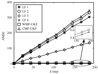 图 2 局部UKF, WMF-UKF以及CMF-UKF的AMSE曲线Fig. 2 AMSE curves of local UKF, WMF-UKF and CMF-UKF
例2. 考虑一个带有8传感器的平面跟踪系统, 在笛卡尔坐标下的状态方程和观测方程如下:
$ {\pmb x}(k+1)=\Phi{\pmb{x}}(k)+ \Gamma {\pmb w}(k) $
(56) $ \begin{array}{l} {\mathit{\boldsymbol{z}}^{(j)}}(k) = {\mathit{\boldsymbol{h}}^{(j)}}(\mathit{\boldsymbol{x}}(k),k) + \mathit{\boldsymbol{v}}_k^{(j)} = \\ \quad \left[ {\begin{array}{*{20}{c}} {\sqrt {{{(x(k) - {x_j})}^2} + {{(y(k) - {y_j})}^2}} }\\ {\arctan \left( {\frac{{y(k) - {y_j}}}{{x(k) - {x_j}}}} \right)} \end{array}} \right] + {\mathit{\boldsymbol{v}}^{(j)}}(k),{\mkern 1mu} \\ \qquad \qquad \qquad \qquad \quad j = 1, \cdots ,8 \end{array} $
(57) 其中, $\mathit{\boldsymbol{x}}(k)={{\left[ x(k)~~\dot{x}(k)~~y(k)~~\dot{y}(k) \right]}^{\text{T}}} $为状态变量, , , ${{\mathit{\boldsymbol{w}}}_{k}} $为零均值, 方差为$\textit{Q}_{w}^{2}={\rm{diag}}\{0.1^{2}, 0.1^{2}\}$的过程噪声.设8个传感器分别放置在4个地点, 其中$l_{1, 2}(5.5, 5)$, $l_{3, 4}(-5, 5.5)$, $l_{5, 6}(-5, -5)$, $l_{7, 8}(5.5, -5.5)$. ${\pmb v}^{(i)}(k)$, ${\pmb v}^{(j)}(k)\ (i\neq j)$互不相关, 且方差分别为.在仿真中, 设采样周期为$T=200\, \rm{ms}$, 状态初值为 $\mathit{\boldsymbol{x}}(0)={{[0\quad 0\quad 0\quad 0]}^{\text{T}}} $.
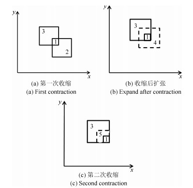
经测试, 本例选取Gauss-Hermite系数$\gamma=1.04$.为了减少计算量, 本例将目标移动范围划分成了16个1平方公里的子区域, 如图 3(a)所示.每个子区域采用以该区域为中心, 外扩2点的方法避免边缘拟合效果不良.以子区域7为例, 以点(0, 0), (0, 1), (1, 1)和(1, 0)所围区域为中心, 外扩2点得到该子区域的拟合采样点如图 3(b)所示.计算该区域的系数矩阵$\overline{H}^{(0)}$, $\overline{M}$和$\overline{H}^{(\rm{I})}$, 如图 3(c)所示.不难看出, 由于8个传感器位于4个点, 这里至少可以将16维的集中式融合观测方程 ${{\mathit{\boldsymbol{h}}}^{(0)}}(\mathit{\boldsymbol{x}}(k),k) $压缩成8维的加权观测融合方程.将16个区域对应的$\overline{M}$和$\overline{H}^{(\rm{I})}$与中介函数$\mathit{\boldsymbol{\overline \psi }} (\mathit{\boldsymbol{x}}(k), k)$离线计算存储并形成数据库.根据每时刻状态预报, 在数据库中选取相应的$\overline{M}$, $\overline{H}^{(\rm{I})}$以及$\mathit{\boldsymbol{\overline \psi }} (\mathit{\boldsymbol{x}}(k), k)$可减少在线计算负担.
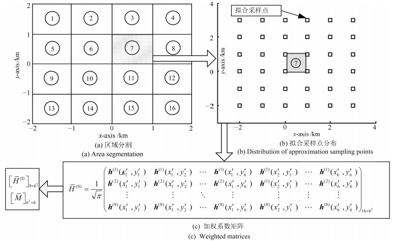 图 3 加权系数矩阵$\overline{M}$和$\overline{H}^{(\rm{I})}$的计算Fig. 3 Calculation of the weighted matrices $\overline{M}$ and $\overline{H}^{(\rm{I})}$
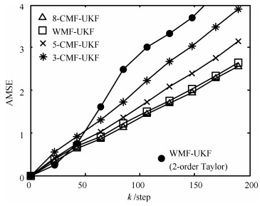
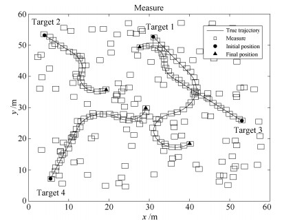
为了对比分析WMF-UKF的精度和计算量, 本文选取了8传感器集中式融合UKF(8-CMF-UKF), 5传感器集中式融合UKF(5-CMF-UKF)以及3传感器集中式融合UKF(3-CMF-UKF).传感器的选择原则是尽量的分散, 例如, 3-CMF-UKF选择的是1, 3和5传感器, 5-CMF-UKF选择的是1, 3, 5, 7和8传感器.各种融合系统的滤波跟踪轨迹曲线如图 4所示.
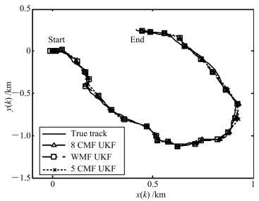 图 4 真实轨迹和WMF-UKF, 8-CMF-UKF和5-CMF-UKF的估计曲线Fig. 4 True and estimated tracks using WMF-UKF, 8-CMF-UKF and 5-CMF-UKF
本例采用$k$时刻位置$(x(k), y(k))$的累积均方误差(AMSE)作为指标函数, 如式(58)所示.
$ \begin{align} \rm{AMSE}(k)=\,&\sum_{t=0}^{k}\frac{1}{N}\sum_{i=1}^{N}\left((x^{i}(t)-\hat{x}^{i}(t|t)\right)^{2}+\notag\\ &\left(y^{i}(t)-\hat{y}^{i}(t|t))^{2}\right) \end{align} $
(58) 其中, $(x^{i}(t), y^{i}(t))$是$t$时刻第$i$次Monte Carlo实验的真实值, $(\hat{x}^{i}(t|t), \hat{y}^{i}(t|t))$是$t$时刻第$i$次Monte Carlo实验的估计值.独立进行20次Monte Carlo实验, 得到的AMSE曲线如图 5所示.
在精度方面, 由图 5可以看到AMSE由低到高依次是8-CMF-UKF, WMF-UKF, 5-CMF-UKF和3-CMF-UKF.实验说明, 随着传感器数量的增加, 集中式融合算法的精度不断提高, 而本文提出的WMF-UKF算法的精度接近全观测集中式融合8-CMF-UKF.
在计算量方面, 加权观测融合系统观测方程为8维, 因此时间复杂度为$\rm O(8^{3})$. 3传感器集中式融合系统观测方程为6维, 因此时间复杂度为$\rm O(6^{3})$. 5传感器集中式融合系统观测方程为10维, 因此时间复杂度为$\rm O(10^{3})$. 8传感器集中式融合系统观测方程为16维, 因此时间复杂度为$\rm O(16^{3})$.因此, 时间复杂度由高到低依次为: 8-CMF-UKF, 5-CMF-UKF, WMF-UKF和3-CMF-UKF.
此外, 为了比较分析, 本例应用文献[25]中的Taylor级数逼近方法得到的WMF-UKF的AMSE曲线也绘于图 5中, 这里我们采用2阶Taylor级数逼近.由于Taylor级数展开阶数以及展开点等原因, 使得其精度低于其他融合算法.而且与本文的不需要在线计算融合矩阵的WMF-UKF算法相比, 文献[25]的WMF-UKF (2-order Taylor)算法需要根据在线预报值实时计算融合参数矩阵, 因而具有更大的在线计算负担.
本例根据不同Hermite多项式$(p=0, 2, 4)$情形进行了仿真分析.经离线测试, 选取Gauss-Hermite系数分别为: $\gamma=0.83\, (p=0), \, \gamma=1.04(p=2), \, \gamma=1\, (p=4), \, $其他参数不变.得到Monte Carlo实验的AMSE曲线如图 6所示.图 6中可以看到, Hermite多项式的数量与函数逼近效果并无直接关系, 得到融合估值精度间也不存在渐近最优性.因此, 根据被逼近函数形式, 离线测试逼近函数效果, 对本文所提出WMF-UKF算法的精度起到非常关键的作用.
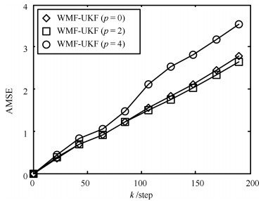 图 6 带不同Hermite多项式的WMF-UKF位置AMSE曲线Fig. 6 AMSE curves of WMF-UKFs with different Hermite polynomials for position
综上, 合理的选择Gauss-Hermite逼近函数以及相应的系数$\gamma$, 可使本文提出的WMF-UKF在精度方面接近集中式融合算法, 而减少计算量.
6. 结论
本文首先基于Gauss-Hermite逼近方法和加权最小二乘法, 提出了一种具有普适性的非线性加权观测融合算法.进而结合UKF算法, 提出了非线性加权观测融合UKF (WMF-UKF)算法.与CMF-UKF算法相比, WMF-UKF具有与之逼近的估计精度, 但计算量明显降低, 并且随着传感器数量的增加, 该算法在计算量上的优势将更加明显.本文通过仿真实例对比已有的相关算法, 说明了本算法的有效性.
-
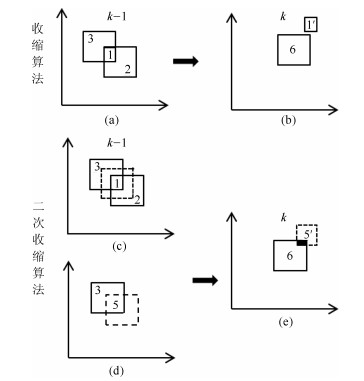
图 2 传统收缩算法和二次收缩算法下箱粒子状态更新
Fig. 2 The box particle state update by using the traditional contraction algorithm and the quadratic contraction algorithm, respectively

图 4 IMM-Box-LMB算法对目标状态估计与目标航迹跟踪效果
Fig. 4 True trajectories and estimates of targets using the IMM-Box-LMB algorithm
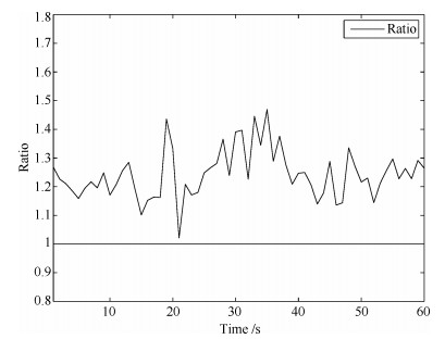
图 5 IMM-Box-LMB算法使用二次收缩算法和传统收缩算法更新之后的有效箱粒子数的比值(50 MC)
Fig. 5 Count the number of effective box particles for IMM-Box-LMB algorithm using the quadratic contraction algorithm and the traditional contraction algorithm, respectively, and then return to their ratio (50 MC)
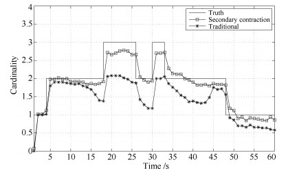
图 6 IMM-Box-LMB算法使用二次收缩算法和传统收缩算法对多机动目标的势估计(50 MC)
Fig. 6 Cardinality statistics returned by IMM-Box-LMB algorithm using the traditional contraction algorithm and the quadratic contraction algorithm, respectively (50 MC)

图 7 IMM-Box-LMB算法使用二次收缩算法和传统收缩算法之后(a) OSPA距离和OSPA成分(b)位置和(c)势估计$p = 1$, $c = 5$ (50 MC)
Fig. 7 The OSPA of IMM-Box-LMB algorithm using the traditional contraction algorithm and the quadratic contraction algorithm, respectively. (a) OSPA distance and OSPA components (b) localization component (c) cardinality component $p=1$, $c = 5$ (50MC)
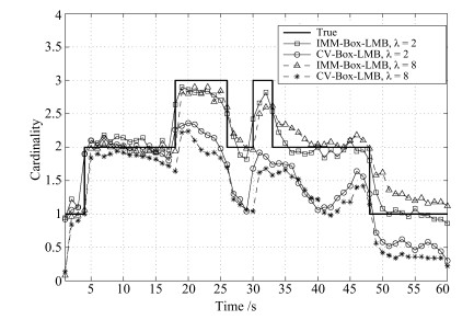
图 8 IMM-Box-LMB, CV-Box-LMB不同杂波率下目标个数估计(50 MC)
Fig. 8 IMM-Box-LMB, CV-Box-LMB cardinality estimates under different clutter rates (50 MC)
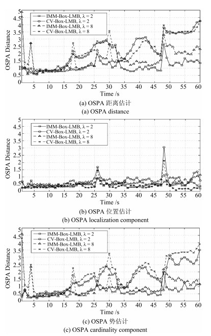
图 9 不同杂波率下IMM-Box-LMB算法和CV-Box-LMB算法OSPA距离(a)和OSPA成分位置(b)和势(c)估计$p = 1$, $c = 5$ (50 MC)
Fig. 9 Under different clutter rates, (a) The OSPA distance and OSPA components. (b) localization component (c) cardinality component $(p = 1, c = 5)$ using IMM-Box-LMB algorithm and CV-Box-LMB algorithm, respectively (50 MC)
-
[1] Blackman S S. Multiple hypothesis tracking for multiple target tracking. IEEE Aerospace and Electronic Systems Magazine, 2004, 19(1): 5-18 [2] Chang K C, Bar-Shalom Y. Joint probabilistic data association for multitarget tracking with possibly unresolved measurements and maneuvers. IEEE Transactions on Automatic Control, 1984, 29(7): 585-594 http://www.wanfangdata.com.cn/details/detail.do?_type=perio&id=6a84b10cd4663c41e72d499a60b0cf3d [3] Mahler R P S. Statistical Multisource-Multitarget Information Fusion. London: Artech House, 2007. 565-682 [4] Mahler R P S. Multitarget Bayes filtering via first-order multitarget moments. IEEE Transactions on Aerospace and Electronic Systems, 2003, 39(4): 1152-1178 http://www.wanfangdata.com.cn/details/detail.do?_type=perio&id=1de4826f6f0ff5b11dbc1832d7b3a490 [5] Mahler R. PHD filters of higher order in target number. IEEE Transactions on Aerospace and Electronic Systems, 2007, 43(4): 1523-1543 http://www.wanfangdata.com.cn/details/detail.do?_type=perio&id=e917996c66d0f95baad191a9741e30df [6] Mahler R P S. Statistical Multisource-Multitarget Information Fusion. London: Artech House, 2007. 110-120 [7] Vo B T, Vo B N, Cantoni A. The cardinality balanced multi-target multi-Bernoulli filter and its implementations. IEEE Transactions on Signal Processing, 2009, 57(2): 409-423 http://www.wanfangdata.com.cn/details/detail.do?_type=perio&id=61dfd7f286ae58058d68670341ea1672 [8] Vo B T, Vo B N. Labeled random finite sets and multi-object conjugate priors. IEEE Transactions on Signal Processing, 2013, 61(13): 3460-3475 [9] Vo B N, Vo B T, Phung D. Labeled random finite sets and the Bayes multi-target tracking filter. IEEE Transactions on Signal Processing, 2014, 62(24): 6554-6567 [10] Reuter S, Vo B T, Vo B N, Dietmayer K. The labeled multi-Bernoulli filter. IEEE Transactions on Signal Processing, 2014, 62(12): 3246-3260 [11] Papi F, Vo B N, Vo B T, Fantacci C, Beard M. Generalized labeled multi-Bernoulli approximation of multi-object densities. IEEE Transactions on Signal Processing, 2015, 63(20): 5487-5497 http://www.wanfangdata.com.cn/details/detail.do?_type=perio&id=69f387345082d430d7add445f6c3c32c [12] 邱昊, 黄高明, 左炜, 高俊.多模型标签多伯努利机动目标跟踪算法.系统工程与电子技术, 2015, 37(12): 2683-2688 http://www.wanfangdata.com.cn/details/detail.do?_type=perio&id=xtgcydzjs201512003Qiu Hao, Huang Gao-Ming, Zuo Wei, Gao Jun. Multiple model labeled multi-Bernoulli filter for maneuvering target tracking. Systems Engineering and Electronics, 2015, 37(12): 2683-2688 http://www.wanfangdata.com.cn/details/detail.do?_type=perio&id=xtgcydzjs201512003 [13] 袁常顺, 王俊, 向洪, 孙进平.基于VB近似的自适应$\delta$-GLMB滤波算法.系统工程与电子技术, 2017, 39(2): 237-243Yuan Chang-Shun, Wang Jun, Xiang Hong, Sun Jin-Ping. Adaptive $\delta$-GLMB filtering algorithm based on VB approximation. Systems Engineering and Electronics, 2017, 39(2): 237-243 [14] 朱书军, 刘伟峰, 崔海龙.基于广义标签多伯努利滤波的可分辨群目标跟踪算法.自动化学报, 2017, 43(12): 2178-2189 doi: 10.16383/j.aas.2017.c160334Zhu Shu-Jun, Liu Wei-Feng, Cui Hai-Long. Multiple resolvable groups tracking using the GLMB filter. Acta Automatica Sinica, 2017, 43(12): 2178-2189 doi: 10.16383/j.aas.2017.c160334 [15] Reuter S, Scheel A, Dietmayer K. The multiple model labeled multi-Bernoulli filter. In: Proceedings of the 18th International Conference on Information Fusion. Washington, DC, USA: IEEE, 2015. 1574-1580 [16] Abdallah F, Gning A, Bonnifait P. Box particle filtering for nonlinear state estimation using interval analysis. Automatica, 2008, 44(3): 807-815 http://www.wanfangdata.com.cn/details/detail.do?_type=perio&id=4f54944c69790e29fab9581937904202 [17] Jaulin L, Kieffer M, Didrit O, Walter É. Applied Interval Analysis. London: Springer, 2001. 11-43 [18] Luc Jaulin. Computing minimal-volume credible sets using interval analysis; application to bayesian estimation. IEEE Transactions on Signal Processing, 2006, 54(9): 3632-3636 http://www.wanfangdata.com.cn/details/detail.do?_type=perio&id=0c257c984c945138181d145de20b15b5 [19] 苗雨, 宋骊平, 姬红兵.箱粒子广义标签多伯努利滤波的目标跟踪算法.西安交通大学学报, 2017, 51(10): 107-112 http://www.wanfangdata.com.cn/details/detail.do?_type=perio&id=xajtdxxb201710018Miao Yu, Song Li-Ping, Ji Hong-Bing. Target tracking method with box-particle generalized label multi-Bernoulli filtering. Journal of Xi'an Jiaotong University, 2017, 51(10): 107-112 http://www.wanfangdata.com.cn/details/detail.do?_type=perio&id=xajtdxxb201710018 [20] 魏帅, 冯新喜, 王泉, 鹿传国.基于箱粒子滤波的鲁棒标签多伯努利跟踪算法.兵工学报, 2017, 38(10): 2062-2068 http://www.wanfangdata.com.cn/details/detail.do?_type=perio&id=bgxb201710024Wei Shuai, Feng Xin-Xi, Wang Quan, Lu Chuan-Guo. Robust labeled multi-Bernoulli tracking algorithm based on box particle filtering. Acta Armamentarii, 2017, 38(10): 2062-2068 http://www.wanfangdata.com.cn/details/detail.do?_type=perio&id=bgxb201710024 [21] Mazor E, Averbuch A, Bar-Shalom Y, Dayan J. Interacting multiple model methods in target tracking: a survey. IEEE Transactions on Aerospace and Electronic Systems, 1998, 34(1): 103-123 [22] Ristic B, Arulampalam S, Gordon N. Beyond the Kalman Filter: Particle Filters for Tracking Applications. London: Artech House, 2004. 24-28 [23] Boers Y, Driessen J N. Interacting multiple model particle filter. IEE Proceedings - Radar, Sonar and Navigation, 2003, 150(5): 344-349 [24] Ristic B, Vo B N, Clark D, Vo B T. A metric for performance evaluation of multi-target tracking algorithms. IEEE Transactions on Signal Processing, 2011, 59(7): 3452-3457 期刊类型引用(0)
其他类型引用(2)
-


 下载:
下载:
 下载:
下载:
计量
- 文章访问数: 1275
- HTML全文浏览量: 152
- PDF下载量: 147
- 被引次数: 2
