

-
摘要: 张量指数函数已经广泛应用于工程领域.本文得到了一种有效的张量广义逆, 并以此为基础构造了广义逆张量Padé逼近的一种$\varepsilon$-算法.该算法可以编程实施递推的计算, 其特点是, 在计算过程中, 不必计算张量的乘积, 也不必计算张量的逆.给出的计算张量指数函数的数值实验显示, 将本文的方法与目前通常使用的截断法进行比较, 在不降低逼近阶的条件下, $\varepsilon$-算法能很好地降低计算复杂度, 尤其是在张量的维数比较大的时候.
-
关键词:
- 张量指数函数 /
- 广义逆张量Padé逼近 /
- 张量$\varepsilon$-算法 /
- 张量指数函数的截断法
Abstract: Tensor exponent functions have been widely used in engineering. In this paper, an effective tensor generalized inverse is obtained, and based on it, an $\varepsilon$-algorithm of generalized inverse tensor Padéapproximation is presented. The algorithm can be programmed to implement recursive calculations, which are characterized by the fact that it is not necessary to calculate the product of the tensors in the calculation nor to calculate the inverse of tensors. The numerical experiment of calculating tensor exponential function shows that compared with the commonly used truncation method, the $\varepsilon$-algorithm can reduce computational complexity well without reducing the approximation order, especially when the dimension of tensor is relatively large.-
Key words:
- Tensor exponential functions /
- generalized inverse tensor Pad$\acute{e}$ approximation /
- tensor $\varepsilon$-algorithm /
- truncation method
1) 本文责任编委 黎铭 -
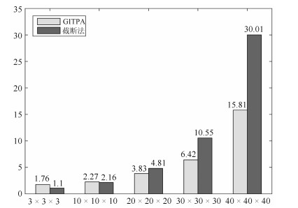
图 1 不同维数下两种算法运行时间直方图(s)
Fig. 1 The time-consuming comparison histogram of two algorithms in different dimensions (s)
表 1 $[\frac{4}{4}]$型GITPA-算法数值实验
Table 1 The numerical experiment of $[\frac{4}{4}]$ type GITPA-algorithm
$x$ $(1, 2, 1)$ $(2, 2, 1)$ $(1, 2, 2)$ $(2, 2, 2)$ $ RES $ 0.2 $E$值 0.08766299 0.87955329 0.12044671 -0.08766299 $5.69\times10^{-13}$ $A$值 0.08766327 0.87955283 0.12044717 -0.08766327 0.4 $E$值 0.15420167 0.78130960 0.21869040 -0.15420167 $3.74\times10^{-10}$ $A$值 0.15420895 0.78129804 0.21870196 -0.15420895 0.6 $E$值 0.20408121 0.70078192 0.29921808 -0.20408121 $1.40\times10^{-8}$ $A$值 0.20412606 0.70071136 0.29928864 -0.20412606 0.8 $E$值 0.24081224 0.63444735 0.36555265 -0.24081224 $1.63\times10^{-7}$ $A$值 0.24096630 0.63420702 0.36579298 -0.24096630 1 $E$值 0.26715410 0.57953894 0.42046106 -0.26715410 $1.01\times10^{-6}$ $A$值 0.26753925 0.57894247 0.42105753 -0.26753925  下载: 导出CSV
表 2 算法1和算法2的数值实验比较
Table 2 The numerical experiment comparison of Algorithm 1 and Algorithm 2
$[\frac{j+2k}{2k}]$ 张量$\varepsilon$-算法 $n_{\rm{max}}$ $\sum^{n_{\rm{max}}}_{n=0}\frac{1}{n!}\mathcal{A}^nt^n $ $a_{121}$ $a_{221}$ $a_{122}$ $a_{222}$ $a_{121}$ $a_{221}$ $a_{122}$ $a_{222}$ $[\frac{2}{2}]$ 0.4235 0.3513 0.6487 -0.4235 1 1.0000 -0.3333 1.3333 -1.0000 $[\frac{4}{4}]$ 0.3049 0.4141 0.5859 -0.3049 2 -0.3333 1.0556 -0.0556 0.3333 $[\frac{6}{6}]$ 0.3098 0.4068 0.5932 -0.3098 3 0.7222 -0.0062 1.0062 -0.7222 - - - - 4 0.1049 0.6116 0.3884 -0.1049 - - - - 5 0.3931 0.3234 0.6766 -0.3931 - - - - 6 0.2810 0.4355 0.5645 -0.2810 - - - - 7 0.3184 0.3981 0.6019 -0.3184 - - - - 8 0.3075 0.4090 0.5910 -0.3075 - - - - 9 0.3103 0.4062 0.5938 -0.3103 - - - - 10 0.3097 0.4069 0.5931 -0.3097 - - - - 11 0.3098 0.4067 0.5933 -0.3098 - - - - 12 0.3098 0.4068 0.5932 -0.3098
下载: 导出CSV
表 3 算法1和算法2的计算复杂度分析
Table 3 The analysis of computational complexity of Algorithm 1 and Algorithm 2
计算一次 $\varepsilon$-算法: $[\frac{6}{6}]$型 截断法:取13项 复杂度 计算 计算 $t$-积运算 $l^3n^2$ 5 11 数乘运算 $l^2n$ 21 12 范数运算 $l^2n$ 21 0 总和 $5l^3n^2+42l^2n$ $11l^3n^2+12l^2n$
下载: 导出CSV
表 4 不同维数下两种算法的运行时间表(s)
Table 4 The consuming time of two algorithms in different dimensions (s)
张量维数 张量$\varepsilon$-算法运行时间 截断法运行时间 $ 3~\times ~3\times ~3$ 1.755262 1.103832 $10\times 10\times 10$ 2.272663 2.164860 $20\times 20\times 20$ 3.831094 4.805505 $30\times 30\times 30$ 6.419004 10.545785 $40\times 40\times 40$ 15.814063 30.012744
下载: 导出CSV
-
[1] 陈伟宏, 安吉尧, 李仁发, 李万里.深度学习认知计算综述.自动化学报, 2017, 43(11): 1886-1897 doi: 10.16383/j.aas.2017.c160690Chen Wei-Hong, An Ji-Yao, Li Ren-Fa, Li Wan-Li. Review on deep-learning-based cognitive computing. Acta Automatica Sinica, 2017, 43(11): 1886-1897 doi: 10.16383/j.aas.2017.c160690 [2] 王守辉, 于洪涛, 黄瑞阳, 马青青.基于模体演化的时序链路预测方法.自动化学报, 2016, 42(5): 735-745 doi: 10.16383/j.aas.2016.c150526Wang Shou-Hui, Yu Hong-Tao, Huang Rui-Yang, Ma Qing-Qing. A temporal link prediction method based on motif evolution. Acta Automatica Sinica, 2016, 42(5): 735-745 doi: 10.16383/j.aas.2016.c150526 [3] 胡扬, 张东波, 段琪.目标鲁棒识别的抗旋转HDO局部特征描述.自动化学报, 2017, 43(4): 665-673 doi: 10.16383/j.aas.2017.c150837Hu Yang, Zhang Dong-Bo, Duan Qi. An improved rotation-invariant HDO local description for object recognition. Acta Automatica Sinica, 2017, 43(4): 665-673 doi: 10.16383/j.aas.2017.c150837 [4] 林洪彬, 邵艳川, 王伟.二维解析张量投票算法研究.自动化学报, 2016, 42(3): 472-480 doi: 10.16383/j.aas.2016.c150339Lin Hong-Bin, Shao Yan-Chuan, Wang Wei. The 2D analytical tensor voting algorithm. Acta Automatica Sinica, 2016, 42(3): 472-480 doi: 10.16383/j.aas.2016.c150339 [5] Batselier K, Chen Z M, Wong N. A tensor network Kalman filter with an application in recursive MIMO Volterra system identification. Automatica, 2017, 84: 17-25 http://www.wanfangdata.com.cn/details/detail.do?_type=perio&id=c6be6022161902761f946caca86046f8 [6] Liu X D, Yu Y, Li Z, Iu H H C, Fernando T. An efficient algorithm for optimally reshaping the TP model transformation. IEEE Transactions on Circuits and Systems Ⅱ: Express Briefs, 2017, 64(10): 1187-1191 [7] Lee C S. Human action recognition using tensor dynamical system modeling. In: Proceedings of the 2017 IEEE Conference on Computer Vision and Pattern Recognition Workshops. Honolulu, HI, USA: IEEE, 2017. 1935-1939 [8] Koniusz P, Cherian A, Porikli F. Tensor representations via kernel linearization for action recognition from 3D skeletons. In: Proceedings of European Conference on Computer Vision. Cham, Switzerland: Springer, 2016. 37-53 [9] De Souza Neto E A. The exact derivative of the exponential of an unsymmetric tensor. Computer Methods in Applied Mechanics and Engineering, 2001, 190(18-19): 2377-2383 http://www.wanfangdata.com.cn/details/detail.do?_type=perio&id=33736cc2a5a29e32d5f7eec4a2ef5aaa [10] de Souza Neto E A, Perić D, Owen D R J. Computational Methods for Plasticity: Theory and Applications. United Kingdom: Wiley, 2008. [11] Kolda T G, Bader B W. Tensor decompositions and applications. SIAM Review, 2009, 51(3): 455-500 http://d.old.wanfangdata.com.cn/NSTLQK/NSTL_QKJJ0211023807/ [12] Kilmer M E, Braman K, Hao N, Hoover R C. Third-order tensors as operators on matrices: a theoretical and computational framework with applications in imaging. SIAM Journal on Matrix Analysis and Applications, 2013, 34(1): 148-172 [13] Kilmer M E, Martin C D, Perrone L. A Third-order Generalization of the Matrix SVD as a Product of Third-order Tensors. Tech. Report TR-2008-4, Tufts University, USA, 2008 [14] Graves-Morris P R. Vector valued rational interpolants I. Numerische Mathematik, 1983, 41(3): 331-348 http://d.old.wanfangdata.com.cn/Periodical/sxyjypl200803028 [15] Gu C Q. Generalized inverse matrix Padé approximation on the basis of scalar products. Linear Algebra and its Applications, 2001, 322(1-3): 141-167 [16] Gu C Q. A practical two-dimensional thiele-type matrix Padé approximation. IEEE Transactions on Automatic Control, 2003, 48(12): 2259-2263 [17] 顾传青.关于矩阵指数的Padé逼近新算法.自动化学报, 1999, 25(1): 94-99 http://www.aas.net.cn/article/id/16737Gu Chuan-Qing. New algorithm for matrix exponentials by Padé approximation. Acta Automatica Sinica, 1999, 25(1): 94-99 http://www.aas.net.cn/article/id/16737 [18] Gu Chuan-Qing. Matrix $\varepsilon$-algorithm and $\eta$-algorithm for Samelson inverse and application to matrix exponentials. Journal on Numerical Methods and Computer Applications, 1999, 20(3): 223-230 -

 下载:
下载:

计量
- 文章访问数: 2699
- HTML全文浏览量: 638
- PDF下载量: 124
- 被引次数: 0
