

-
摘要: 在作为人工智能核心技术的机器学习领域,强化学习是一类强调机器在与环境的交互过程中进行学习的方法,其重要分支之一的自适应评判技术与动态规划及最优化设计密切相关.为了有效地求解复杂动态系统的优化控制问题,结合自适应评判,动态规划和人工神经网络产生的自适应动态规划方法已经得到广泛关注,特别在考虑不确定因素和外部扰动时的鲁棒自适应评判控制方面取得了很大进展,并被认为是构建智能学习系统和实现真正类脑智能的必要途径.本文对基于智能学习的鲁棒自适应评判控制理论与主要方法进行梳理,包括自学习鲁棒镇定,自适应轨迹跟踪,事件驱动鲁棒控制,以及自适应H∞控制设计等,并涵盖关于自适应评判系统稳定性、收敛性、最优性以及鲁棒性的分析.同时,结合人工智能、大数据、深度学习和知识自动化等新技术,也对鲁棒自适应评判控制的发展前景进行探讨.Abstract: In the machine learning field, the core technique of artificial intelligence, reinforcement learning is a class of strategies focusing on learning during the interaction process between machine and environment. As an important branch of reinforcement learning, the adaptive critic technique is closely related to dynamic programming and optimization design. In order to effectively solve optimal control problems of complex dynamical systems, the adaptive dynamic programming approach was proposed by combining adaptive critic, dynamic programming with artificial neural networks and has been attracted extensive attention. Particularly, great progress has been obtained on robust adaptive critic control design with uncertainties and disturbances. Now, it has been regarded as a necessary outlet to construct intelligent learning systems and achieve true brain-like intelligence. This paper presents a comprehensive survey on the learning-based robust adaptive critic control theory and methods, including self-learning robust stabilization, adaptive trajectory tracking, event-driven robust control, and adaptive H∞ control design. Therein, it covers a general analysis for adaptive critic systems in terms of stability, convergence, optimality, and robustness. In addition, considering novel techniques such as artificial intelligence, big data, deep learning, and knowledge automation, it also discusses future prospects of robust adaptive critic control.
-
Key words:
- Adaptive critic control /
- intelligent learning /
- neural networks /
- robust control /
- uncertain systems
-
人工智能的发展规划已经上升到国家战略层面, 成为建设科技强国和引领未来的重要技术.备受瞩目的AlphaGo [1]就是人工智能和深度学习技术[2-3]相结合的产物, 其中, 局势评估与落棋位置选择是AlphaGo取得成功的关键环节.人工神经网络[4]的深度学习能力, 树搜索以及强化学习技术[5]三者的融合, 确保程序运行中评估的准确性和决策的最优性.最近, 新版程序AlphaGo Zero [6]的出现更被认为是深度强化学习技术的运用典范.
机器学习是人工智能的核心技术, 它是使计算机具有智能的根本途径.作为机器学习领域的重要分支, 强化学习关注机器在与环境的交互中进行智能学习.它研究智能体如何在环境中采取行动, 以最大限度地增加累计奖励或尽量减少惩罚, 其中涉及到最优化思想.事实上, 对于模仿自然和设计自动控制系统的兴趣, 促使人们利用有限资源实现所需的最优性能, 从而使得控制系统达到一定意义下的最优效果.动态规划是一种求解最优化问题的有效计算技术, 通过倒序搜索并利用最优性原理得到最优策略[7-8].然而, 状态和控制维数增大时导致的"维数灾"问题[7], 对于动态系统模型的依赖和倒序搜索与实时控制的矛盾, 极大地限制了该方法的应用范围.虽然如此, 动态规划与强化学习却是密切相关的, 并为理解强化学习思想提供了必要的基础.在强化学习的众多算法中, 有一类自适应评判方法, 它以执行-评判结构为基本框架, 执行组件产生控制行为(或控制律), 评判组件评估该控制行为的价值.自适应评判, 动态规划和神经网络相结合, 产生了用于求得近似最优解的自适应/近似动态规划(Adaptive/approximate dynamic programming, ADP)方法.该方法由Werbos博士首先提出[9-11], 其核心思想是基于自适应评判的优化, 并被认为是实现真正类脑智能的必要途径[11].它的基本结构中有三个组成部分, 即评判模块、模型模块和执行模块, 通常都通过神经网络来实现, 分别执行评估、预测和决策的功能[12-14].应当指出, 同神经网络一样, 模糊逻辑也可以用来提供智能学习能力.在ADP方法体系中, 自适应评判融合强化学习提供学习机制, 动态规划蕴含最优性原理提供理论基础, 神经网络作为函数逼近器提供实现手段.特别地, 它是一种基于数据驱动的方法, 具有在线学习与正序求解的能力.在人工智能、类脑智能、大数据、云计算、物联网等新技术不断涌现的背景下, 具有强大自学习能力的ADP, 符合知识自动化的潮流, 已经成为一种极有发展前景的智能优化技术.
利用ADP方法进行智能优化决策的基础是最优控制设计.关于线性系统的最优调节器设计, 在控制理论和控制工程界已经有很多成熟的方法.然而, 对于一般的非线性系统, 获得Hamilton-Jacobi-Bellman (HJB)方程的解析解并不是一件容易的事情.此类系统的最优控制设计相当困难, 但是却相当重要, 因此引起了人们的广泛重视.其中, 逐次逼近法[15-17]通过寻找HJB方程的近似解来克服这一困难, 并与ADP方法密切相关.简单来说, ADP是一种基于智能学习思想的新兴方法, 可以为复杂动态系统提供有效的优化控制解决方案[9-17].在过去的二十年中, ADP在求解离散时间和连续时间系统的自适应最优控制问题中得到了广泛的应用, 例如文献[18-33].近年来的综述文献和学术专著, 如文献[34-42], 在理论、设计、分析和应用等层面对该领域的研究工作进行了总结.如今, 基于数据驱动的控制设计已经成为控制理论和控制工程领域的研究热点[43-44], ADP能够促进基于数据的决策与优化控制研究, 并有利于人工智能和计算智能技术的发展.
在有关ADP方法的现有结果中, 大多数是在不考虑被控对象不确定性的前提下得到的.但是, 实际中的控制系统总是受着模型不确定性, 外界扰动或其他变化的影响.我们在控制器设计过程中必须考虑这些因素, 以避免闭环系统性能的恶化, 提高被控系统的鲁棒性能.关于不确定系统的鲁棒控制问题, 控制学者们已经取得了很多研究成果, 如文献[45-50]和其中的参考文献.在文献[49-50]中, 作者通过设计标称系统的最优控制器处理鲁棒控制问题.这是在两种控制问题之间建立有效联系的一项重要结果, 但是并没有给出详细的设计步骤, 也很难处理一般的非线性系统.文献[51-52]提出基于HJB方程的非线性系统鲁棒控制器设计方法, 但是求解过程是离线进行的, 而且没有充分讨论闭环系统的稳定性.
近几年来, 利用自适应评判思想进行鲁棒控制设计逐渐成为ADP领域的研究热点之一, 有很多方法陆续被提出, 这里统称为鲁棒自适应评判控制(Robust adaptive critic control).一种基本的做法是进行问题转换, 以建立鲁棒性和最优性之间的密切关系[53-62].在这些文献中, 闭环系统一般满足最终一致有界稳定.这些结果充分表明, ADP方法适用于不确定环境下的复杂非线性系统鲁棒控制设计.由于以前的许多ADP文献并不关注控制器的鲁棒性能, 鲁棒自适应评判控制的出现, 极大地扩大了ADP方法的使用范围.随后, 考虑到在处理系统不确定项方面的共性, 结合ADP和滑模控制技术的自学习优化方法, 为鲁棒自适应评判控制提供了一个新的研究方向[63].另外, 鲁棒ADP方法[64-68], 是该领域的又一重要成果.文献[65]给出了线性和非线性系统鲁棒ADP方法的研究综述.值得一提的是, 鲁棒ADP方法在电力系统中的应用受到了特别关注[64-68].一般而言, 基于鲁棒ADP的控制器不仅能够镇定原始的不确定系统, 而且使得系统在不含有动态不确定性的情况下也能达到最优.总之, 鲁棒自适应评判控制, 包含了关于系统稳定性、收敛性、最优性、鲁棒性的讨论, 在不确定环境下复杂系统的智能学习控制领域扮演着重要角色.本文从一般的自适应评判设计引入主题, 以解决不确定环境下的鲁棒镇定问题为出发点, 着重分析鲁棒自适应评判控制设计的主要方法, 并探讨相关领域的发展趋势.
在本文中, ${\bf R}$代表所有实数集. ${\bf R}^n$表示由所有$n$-维实向量组成的欧氏空间. ${{\bf R}}^{n\times m}$是所有$n\times m$实矩阵组成的空间. $\|\cdot\|$表示在${ \bf R}^n$上的向量范数或者在${{\bf R}}^{n\times m}$上的矩阵范数. $I_{n}$代表$n \times n$维单位矩阵. $\lambda_{\max}(\cdot)$和$\lambda_{\min}(\cdot)$分别表示矩阵的最大和最小特征值. $\text{diag}\{a_{1}, a_{2}, \cdots, a_{n}\}$表示由各元素构成的对角矩阵.令$\Omega$是${{\bf R}}^{n}$的一个紧集, 而$\Omega_{u}$是${\bf R}^m$的一个紧集, 并且$\mathcal{A}(\Omega)$是$\Omega$上所有容许控制律(定义见文献[16-17, 22, 28])的集合. $\rho$是效用函数中对应于不确定项的参数. $\mathcal{L}_{2}[0, \infty)$表示函数空间, 其中元素的Lebesgue积分有界. $\varrho$是$\mathcal{L}_{2}$-增益性能水平. $i$是策略学习算法中的迭代指标, $j$是事件触发机制下的采样时刻. ${\bf N} = \{0, 1, 2, \cdots\}$表示所有非负整数的集合. "${\rm T}$"代表转置操作且$\nabla (\cdot):=\partial (\cdot)/\partial x$是梯度操作符.
1. 基于学习的自适应评判控制设计
本部分包括基本的问题描述与设计思路, 神经网络实现与系统稳定性分析, 以及关于改进自适应评判学习机制的讨论.
1.1 问题描述与设计思路
考虑一类控制输入具有仿射形式的连续时间非线性系统
$$ \begin{align} \label{Eq55004} \dot{x}(t)=f(x(t))+g(x(t))u(t) \end{align} $$ (1) 其中, $x(t)\in \Omega \subset{\bf R}^n$是状态向量, $u(t) \in \Omega_{u} \subset {\bf R}^m$是控制向量.系统函数$f(\cdot)$和$g(\cdot)$可微且$f(0)=0$.令在$t=0$时的初始状态为$x(0)=x_{0}$, 且$x=0$是被控系统的一个平衡点.假设系统函数$f(x)$在属于${\bf R}^n$并且包含原点的集合$\Omega$上是Lipschitz连续的.一般地, 我们假设非线性动态系统(1)能控.
针对有限时域上的无折扣最优控制问题, 令
$$ \begin{align}\label{Eq55013} U(x(t), u(t))=Q(x(t))+u^{\rm T}(t)Ru(t) \end{align} $$ (2) 表示效用函数, 其中$Q(x) \geq 0$为标量函数, $R =R^{\rm T} > 0$为$m$-维方阵, 并且定义代价函数为
$$ \begin{align} \label{Eq55005} J(x(t), u(t))=\int_{t}^{\infty}U(x(\tau), u(\tau))\text{d}\tau \end{align} $$ (3) 为了描述简洁, 文中的代价函数$J(x(t), u(t))$可被写成$J(x(t))$或$J(x)$.我们通常关心的代价函数是从$t=0$开始, 因此记做$J(x(0))=J(x_{0})$.如果考虑含有折扣因子$\gamma$ ($\gamma \geq 0$)的情形, 代价函数通常为
$$ \begin{align} \label{Eq68002} J(x(t), u)=\int_{t}^{\infty}{\rm e}^{-\gamma(\tau-t)}U(x(\tau), u(\tau))\text{d}\tau \end{align} $$ (4) 这里的指数折扣项${\rm e}^{-\gamma(\tau-t)}$与研究离散时间系统最优控制时常用的折扣因子(如文献[18])有着类似的功能.
在最优控制问题中, 我们通过设计最优反馈控制律$u(x)$, 使得代价函数(3)达到最小.对于任意一个容许控制律$u(x)\in \mathcal{A}(\Omega)$, 若代价函数(3)连续可微, 则非线性Lyapunov方程为
$$ \begin{align} \label{Eq55023} 0 = U(x, u(x))+(\nabla J(x))^{\rm T}[f(x)+g(x)u(x)] \end{align} $$ (5) 且$J(0)=0$.如果考虑折扣因子的影响, 该方程变为
$$ \begin{align} \label{EQ68003} 0 = U(x, u)-\gamma J(x)+(\nabla J(x))^{\rm T}(f+gu) \end{align} $$ (6) 定义系统(1)的Hamiltonian为
$$ \begin{align} H(x, &\ u(x), \nabla J(x))= U(x, u(x))+\nonumber\\&\ (\nabla J(x))^{\rm T} [f(x)+g(x)u(x)] \end{align} $$ (7) 利用Bellman最优性原理, 最优代价函数
$$ \begin{align}\label{Eq55011} J^{*}(x)= \min\limits_{u \in \mathcal{A}(\Omega)}\int_{t}^{\infty}U(x(\tau), u(\tau))\text{d}\tau \end{align} $$ (8) 满足HJB方程$\min_{u \in \mathcal{A}(\Omega)}H(x, u(x), \nabla J^{*}(x))=0$.基于最优控制理论, 最优状态反馈控制律为
$$ \begin{align} \label{Eq55006} u^{*}(x) =-\frac{1}{2}R^{-1}g^{\rm T}(x) \nabla J^{*}(x) \end{align} $$ (9) 使用最优控制表达式(9), HJB方程转化为如下形式
$$ \begin{align} \label{Eq55007} 0= &\ U(x, u^{*}(x))+(\nabla J^{*}(x))^{\rm T}[f(x)+g(x)u^{*}(x)]=\nonumber\\&H(x, u^{*}(x), \nabla J^{*}(x)) \end{align} $$ (10) 其中, $J^{*}(0)=0$.需要指出, 为了简洁与一致, 本文对于效用函数$U$, 代价函数$J$, 以及Hamiltonian函数$H$等符号的使用, 针对不同问题不做明显区分, 具体意义在相应的问题描述中可以得知.
如果已知最优代价函数的值, 最优控制律就可以直接求得, 也就是说方程(10)是可解的.然而, 实际情况并非如此.因为很难得到连续时间HJB方程(10)的解析解, 所以获取一般非线性系统的最优控制律(9)并不容易.这就激发人们进行迭代算法的研究, 如提出经典的策略迭代.首先, 构造代价函数序列$\{J^{(i)}(x)\}$和控制序列$\{u^{(i)}(x)\}$, 然后, 从一个初始容许控制律开始进行逐次迭代.策略迭代算法包括基于式(5)的策略评估和基于式(9)的策略更新[5], 而且能够最终收敛到最优代价函数和最优控制律, 即当$i \to \infty$时, $J^{(i)}(x)\to J^{*}(x)$且$u^{(i)}(x)\to u^{*}(x)$.这种收敛性证明已经在文献[17]和里面的参考文献中给出.尽管如此, 得到Lyapunov方程的精确解仍然是困难的.于是, 人们提出一类近似方法来克服这一难题[34-39, 41-42].这就促使基于ADP方法的神经控制设计的产生与发展.除此之外, 上述迭代过程往往依赖系统的动态信息$f(x)$和$g(x)$.事实上, 近年来出现的一些方法已经放松了这一要求, 如积分策略迭代算法[28]、神经网络辨识方法[55]和探测信号方法[66], 而且关于这一主题的研究还在进一步深入.这也符合数据驱动控制与学习系统设计的发展趋势.
1.2 神经网络实现与稳定性分析
在自适应评判设计中, 往往需要构建不同类型的神经网络.虽然具体实施过程中可能涉及多种模块, 比如模型网络[18]和执行网络[18, 22], 但是, 评判网络是最重要的模块.不同的模块配置反映控制器设计者的不同目标.其中, 具有单一评判网络结构的处理方法, 主要强调设计过程的简易性[53, 56].
在神经网络实现中, 我们考虑通用逼近性质, 将最优代价函数$J^{*}(x)$在紧集$\Omega$上表示为
$$ \begin{align}\label{Eq49002} J^{*}(x)=\omega_{c}^{\rm T}\sigma_{c}(x)+\varepsilon_{c}(x) \end{align} $$ (11) 其中, $\omega_{c}\in {\bf R}^{l_c}$是理想的权值向量, $l_c$是隐含层神经元个数, $\sigma_{c}(x)\in {\bf R}^{l_c}$是激活函数, $\varepsilon_{c}(x)\in {\bf R}$是重构误差.对于一般的非线性情形, 理想权值向量$\omega_{c}$和重构误差$\varepsilon_{c}$是未知的, 但均有界.易知, 最优代价函数的梯度是$\nabla J^{*}(x)=(\nabla \sigma_{c}(x))^{\rm T}\omega_{c}+\nabla \varepsilon_{c}(x) $.由于理想权值是未知的, 我们构建一个评判神经网络
$$ \begin{align} \label{Eq55019}\hat{J}^{*}(x)=\hat{\omega}_{c}^{\rm T}\sigma_{c}(x) \end{align} $$ (12) 来逼近最优代价函数, 其中$\hat{\omega}_{c}\in {\bf R}^{l_c}$表示估计的权值向量.类似地, 梯度向量为$\nabla \hat{J}^{*}(x)=(\nabla \sigma_{c}(x))^{\rm T}\hat{\omega}_{c} $.
需要指出的是, 评判网络的具体结构往往通过实验选择, 并根据工程经验和直觉确定, 需要在控制精度和计算复杂度之间进行权衡[17].
考虑反馈表达式(9)和神经网络表达式(11), 最优控制律可以写成与权值相关的形式
$$ \begin{align} \label{Eq36009} u^*(x) = -\frac{1}{2}R^{-1} g^{\rm T} (x) \big[(\nabla \sigma_{c}(x))^{\rm T} \omega_{c} + \nabla \varepsilon_{c}(x)\big] \end{align} $$ (13) 利用评判网络(12), 近似的最优反馈控制函数为
$$ \begin{align} \label{Eq55008} \hat{u}^*(x)=-\frac{1}{2}R^{-1}g^{\rm T}(x)(\nabla \sigma_{c}(x))^{\rm T}\hat{\omega}_{c} \end{align} $$ (14) 基于神经网络描述, 近似的Hamiltonian为
$$ \begin{align}\label{Eq0221} \hat H (x, &\ \hat{u}^*(x), \nabla \hat{J}^{*}(x)) = U(x, \hat{u}^*(x))+ \nonumber\\ &\ \hat \omega_c^{\rm T}\nabla \sigma_c(x) [f(x)+g(x)\hat{u}^*(x)] \end{align} $$ (15) 根据式(10)和式(15)定义误差量$e_c=\hat H (x, \nabla \hat{J}^{*}(x)) -H(x, \nabla J^{*}(x))$, 也即$e_{c} = \hat H (x, \hat{u}^*(x), \nabla \hat{J}^{*}(x))$成立.为了训练评判网络使得目标函数$E_{c}=0.5e_{c}^{2}$最小化, 一般采用经典的梯度下降法:
$$ \begin{align} \label{Eq55001} \dot{\hat{\omega}}_{c}=-\alpha_{c}\bigg(\frac{\partial E_{c}}{\partial \hat{\omega}_{c}}\bigg) \end{align} $$ (16) 来调整权值向量, 其中, 常数$\alpha_{c}>0$是学习率标量.这里, 通常会引入一个与$l_c$-维向量$\phi = {\partial e_{c}}/{\partial \hat \omega_c} $相关的归一化正项, 以改善学习效果.在引入折扣因子时, 会出现一个与之相关的项$-\gamma\sigma_{c}(x)$, 从而影响梯度下降法的学习过程.进一步地, 定义理想权值与其估计值之间的误差为$\tilde \omega_c= \omega_c-\hat \omega_c$, 则有$\dot{\tilde \omega}_c= -\dot{\hat \omega}_c$, 由此展开可以得到评判网络的权值误差动态.
在自适应评判设计中, 我们旨在确定评判网络的权值参数以近似最优的代价函数.正如传统自适应控制的要求[46], 在自适应评判控制中, 也需要满足一定的持续激励条件.进而, 根据文献[22], 如果近似最优控制律由式(14)给出, 同时评判网络的权值按照式(16)进行训练, 则闭环系统状态向量和评判网络权值误差都将最终一致有界稳定.进一步地, 可以得到:近似最优控制律$\hat{u}^*(x)$能够收敛到其最优值$u^{*}(x)$的一个小邻域内, 而且这个邻域可以通过设定相关参数(如评判网络学习率)使其任意小.
1.3 改进评判网络学习准则
传统的自适应评判控制设计常常依赖初始稳定控制律.但是, 在实际控制工程中, 往往难以获得初始稳定控制律[22, 55, 66-67], 这在一定程度上缩小了ADP方法的应用范围.一般来说, 需要通过试错的办法, 选择一个初始的权值向量来创建一个初始的稳定控制, 然后开始训练过程.否则, 一个不稳定的控制律可能导致闭环系统不稳定.这激励人们努力放宽对于初始条件的限制[26, 54, 69-71].这一重要思想来源于文献[69], 它采用分段函数来减少初始条件和检测稳定性, 但理论证明比较复杂.于是, 我们针对传统的自适应评判框架, 增加一个额外的强化模块, 以改进评判网络学习准则, 实现在线优化调节, 同时能够简化理论分析[58, 72-73].在具体的神经网络实施过程中, 通过选取合适形式的Lyapunov函数$J_{s}(x)$, 例如$J_{s}(x)=0.5x^{\rm T}x$, 可以有助于自适应评判系统学习性能的提高[58, 72-73].文献[73]已经证明在改进学习规则下的闭环系统稳定性.
基于学习的自适应评判控制结构图如图 1所示, 其中, 实线表示信号流线, 虚线表示神经网络反向传播路径, 而神经网络的学习准则是关键设计模块.
在下面的几个部分中, 我们将面向动态系统的不确定因素, 以自适应评判思想为基础, 阐述基于智能学习的鲁棒自适应评判控制设计近些年来的主要成果, 包括自学习鲁棒镇定, 自适应轨迹跟踪, 事件驱动鲁棒控制, 以及自适应$H_{\infty}$控制设计等.
2. 鲁棒自适应评判控制设计
这里介绍不确定环境下非线性系统自学习鲁棒控制设计的主要方法, 包括基于最小二乘的问题转换方法[51-52], 基于自适应评判的问题转化方法[53-60], 基于数据的问题转换方法[61-62], 组合滑模控制方法[63]和鲁棒ADP方法[64-68].在文献[53]中, 针对具有匹配不确定项的连续时间非线性系统, 作者提出一种新颖的策略迭代算法实现自学习鲁棒镇定.随后, 该方法被推广应用于处理具有未知动态[55]和输入约束[56]非线性系统的鲁棒控制问题.值得一提的是, 针对离散时间非线性系统, 文献[57]也给出了鲁棒自适应评判控制设计的初步成果.为了改善评判神经网络的学习规则, 文献[58]建立了实现非线性系统自适应优化控制的改进方法, 并进一步研究了非线性系统的鲁棒镇定问题.此外, 文献[59]还研究了具有非匹配形式不确定项的非线性系统鲁棒控制问题.随后, 文献[60]扩展文献[54]中的方法, 研究同时含有匹配不确定项和外部扰动的鲁棒控制设计.另外, 为了讨论鲁棒控制器的最优性, 文献[61]建立新颖的匹配非线性系统数据驱动鲁棒最优控制方法.通过积分强化学习, 文献[62]研究了一类具有控制约束未知非线性系统的鲁棒自适应控制.
从研究对象来看, 针对特殊匹配形式不确定系统的自学习鲁棒镇定是设计基础, 而文献[51-52, 59, 65-68]研究了具有非匹配不确定项的自适应鲁棒控制设计.最近, 针对具有一般形式不确定项的非线性系统, 文献[74]提出基于改进学习规则的鲁棒自适应评判控制方案, 而文献[75]从问题转化的角度进行神经网络控制设计, 研究对象逐渐广义化.
如果在动态系统(1)中引入不确定项, 我们就必须关注所设计控制器的鲁棒性.考虑一类含有不确定项的连续时间非线性系统
$$ \begin{equation} \label{Eq51003} \dot{x}(t)=f(x(t))+g(x(t))[u(t)+d(x(t))] \end{equation} $$ (17) 其中, 表达式$g(x)d(x)$反映了一种和控制矩阵匹配的动态不确定项.通常假设$d(0)=0$, 以保持$x=0$是被控系统的平衡点.又假设表达式$d(x)$是有界的, 即$\|d(x)\| \ \leq d_{M}(x) $, 这里$d_{M}(x)$是一个已知函数且满足$d_{M}(0)=0$.
考虑不确定非线性系统(17), 为了解决鲁棒镇定问题, 需要设计一个控制律$u(x)$, 使得闭环系统在考虑不确定性的情况下稳定.引入一个正数$\rho$并且指定$Q(x)=\rho d_{M}^{2}(x)$, 鲁棒镇定问题能够通过设计系统(1)的最优控制器进行求解.这里, 代价函数仍然为式(3)的形式, 但是效用函数取为
$$ \begin{align} \label{Eq51001} U(x(t), u(t))= \rho d_{M}^{2}(x(t))+u^{\rm T}(t)Ru(t) \end{align} $$ (18) 值得注意的是, 即使采用改进的效用函数, 最优控制函数却保持不变.考虑系统(1)和基于改进效用函数(18)的代价函数(3), Hamiltonian变为
$$ \begin{align} \label{Eq048} H(x, &\ u(x), \nabla J(x))= \rho d_{M}^{2}(x)+u^{\rm T}(x)Ru(x)+\nonumber\\&\ (\nabla J(x))^{\rm T} [f(x) + g(x)u(x)] \end{align} $$ (19) 基于改进的效用函数(18), 并再次使用最优控制律(9), 得到改进的最优控制问题的HJB方程为
$$ \begin{align} \label{Eq51002} 0=&\ \rho d_{M}^{2}(x)+(\nabla J^{*}(x))^{\rm T}f(x)- \nonumber\\ &\ \frac{1}{4}(\nabla J^{*}(x))^{\rm T}g(x)R^{-1}g^{\rm T}(x)\nabla J^{*}(x) \end{align} $$ (20) 且有$J^{*}(0)=0$.
文献[53]和[58]分别给出了应用近似最优控制律(14)时, 被控对象标称部分(1)和原始不确定系统(17)的最终一致有界稳定性.应该特别注意的是, 在使用近似最优控制律时, 得到闭环系统最终一致有界稳定[58], 这不同于采用精确最优控制律时的渐近稳定结论[53].此外, 文献[54-55, 61]也讨论了鲁棒控制器的最优性.这是通过给系统(1)的最优反馈控制律(9)增加适当的反馈增益$\pi$和定义特殊的代价函数得到的, 其中, 引入反馈增益后的控制律为
$$ \begin{align} \label{Eq55016} \bar{u}(x) = \pi u^{*}(x)=-\frac{1}{2}\pi R^{-1}g^{\rm T}(x) \nabla J^{*}(x) \end{align} $$ (21) 关于反馈增益的取值对于闭环系统稳定性的影响, 已在文献[54-55, 61]中给出.总的来说, 我们应该设计标称系统的最优控制律, 然后实现原始系统的鲁棒镇定, 也就是说, 可以利用自适应评判思想和神经网络技术来设计有效的鲁棒最优控制器.
为了减少对于系统模型的依赖, 积分策略迭代算法[32]也被用来求解基于ADP的鲁棒控制问题[61-62].为此, 我们考虑引入受限探测信号$\vartheta(t)$的非线性系统, 如下所示
$$ \begin{equation} \dot{x}(t)=f(x(t))+g(x(t))[u(t)+\vartheta(t)] \end{equation} $$ (22) 在线积分策略迭代算法从$i=0$开始进行, 并且在每一步迭代中同时求解$\{J^{(i)}(x), u^{(i)}(x)\}$.由于在积分方程中没有出现$f(x)$和$g(x)$, 因此建立了不需要动态模型的数据驱动策略学习方法.
在文献[63]中, 具有混合结构的滑模控制器的表达式为$u=u^{\text{a}}+u^{\text{s}}$, 其中, 前一部分$u^{\text{a}}$是基于ADP的控制律, 用来镇定滑模动态并且保证次优性能, 而后者$u^{\text{s}}$是不连续控制策略, 设计目的是减小干扰的影响和保证滑模面的可达性.该方法融合了滑模控制的思想, 并扩展了文献[53, 55-56, 59-60]中的结果.
鲁棒ADP方法[64-68]是对于具有不确定项的线性和非线性系统经典ADP方法的重要延伸, 它综合了现代非线性控制理论的几种工具, 如鲁棒再设计和反推技术以及非线性小增益定理[76]等关键策略.文献[66]考虑如下形式的一类非线性系统
$$ \dot{\varsigma}=\delta_{\varsigma}(\varsigma, x) $$ (23a) $$ \dot{x}=f(x)+g(x)[u+\delta(\varsigma, x)] $$ (23b) 其中, $\varsigma$是状态变量的不可测部分, $\delta_{\varsigma}$和$\delta$是未知局部Lipschitz函数.这里的设计目标是找到一个在线控制律来镇定原始不确定系统, 并且在不考虑动态不确定因素时(即$\delta=0$且没有$\varsigma$-子系统), 使其成为最小化标称系统代价函数的最优控制律.这里, 鲁棒性是针对不确定系统的, 而最优性则是针对标称系统讨论的.此外, 这种方法也扩展到了具有非匹配动态不确定项的非线性系统[66]和大规模的复杂系统[67-68].文献[67]和[68]分别研究分散大规模系统最优控制和关联系统输出反馈控制问题, 这也使得鲁棒ADP技术更加完善.
3. 自学习鲁棒跟踪控制设计
自适应评判技术在最优调节器设计中取得了重要进展之外, 也常常应用于非线性系统的轨迹跟踪控制问题.以往的很多成果主要是针对确定系统的跟踪控制设计, 没有考虑不确定因素, 如文献[25, 29].近年来, 关于不确定环境下的鲁棒轨迹跟踪, 在一些主流刊物上也报道了一些最新成果[77-79].
考虑一类含有不确定项的连续时间非线性系统
$$ \begin{equation} \label{Eq0201} \dot{x}(t)=f(x(t))+g(x(t))u(t)+\Delta f(x(t)) \end{equation} $$ (24) 其中, $x(t)\in \Omega \subset{ {\bf R}}^n$是状态向量并且$u(t)\in {\bf R}^m$是控制向量, $f(\cdot)$和$g(\cdot)$可微且满足$f(0)=0$, $\Delta f(x)$是不确定项且有$\Delta f(0)=0$.这里, 令$x(0)=x_{0}$为初始状态并且假设不确定项$\Delta f(x)$有界, 即$\|\Delta f(x)\| \ \leq \lambda_{f}(x) $, 其中, 已知函数$\lambda_{f}(x)$满足$\lambda_{f}(0)=0$.
为了研究轨迹跟踪问题, 引入一个参考系统
$$ \begin{align} \label{Eq60001} \dot{r}(t)=\varphi(r(t)) \end{align} $$ (25) 其中, $r(t) \in {\bf R}^n$代表有界的目标轨迹且满足$r(0)=r_{0}$.这里假设$\varphi(r(t))$是一个Lipschitz连续函数同时满足$\varphi(0)=0$.定义轨迹跟踪误差为
$$ \begin{align} \label{Eq60002} z(t)=x(t)-r(t) \end{align} $$ (26) 并且初始误差向量为$z(0)=z_{0}=x_{0}-r_{0}$.联立式(24) ~ (26), 我们可以得到跟踪误差动态为
$$ \begin{align} \label{Eq60003} \dot{z}(t) = f(x(t)) - \varphi(r(t)) + g(x(t))u + \Delta f(x(t)) \end{align} $$ (27) 考虑到$x(t)=z(t)+r(t)$, 系统(27)可以改写为
$$ \begin{align} \label{Eq60004} \dot{z}(t)=&\ f(z(t)+r(t))+g(z(t)+r(t))u(t)-\nonumber\\&\ \varphi(r(t))+\Delta f(z(t)+r(t)) \end{align} $$ (28) 这里, 定义增广状态向量$\xi(t)=[z^{\rm T}(t), r^{\rm T}(t)]^{\rm T} \in {\bf R}^{2n} $且$\xi(0)=\xi_0=[z^{\rm T}_{0}, r^{\rm T}_{0}]^{\rm T}$是它的初始条件, 那么, 基于式(25)和(28), 增广系统动态可以简洁描述为
$$ \begin{align} \label{Eq60005} \dot{\xi}(t)=\mathcal{F}(\xi(t))+\mathcal{G}(\xi(t))u(t)+\Delta \mathcal{F}(\xi(t)) \end{align} $$ (29) 其中, $ \mathcal{F}(\cdot)$和$ \mathcal{G}(\cdot)$是新的系统矩阵和控制矩阵, 而$\Delta \mathcal{F}(\xi)$是新的不确定项.它们的具体形式为
$$ \mathcal{F}(\xi(t))=\left[ \begin{array}{c} f(z(t)+r(t))-\varphi(r(t)) \\ \varphi(r(t)) \\ \end{array} \right] $$ (30a) $$ \mathcal{G}(\xi(t))=\left[ \begin{array}{c} g(z(t)+r(t)) \\ 0_{n \times m} \\ \end{array}\right] $$ (30b) $$ \Delta \mathcal{F}(\xi(t))=\left[ \begin{array}{c} \Delta f(z(t)+r(t)) \\ 0_{n \times 1} \\ \end{array} \right] $$ (30c) 由于
$$ \begin{align} \label{Eq60010}\|\Delta \mathcal{F}(\xi)\| =&\ \|\Delta f(z+r)\| =\|\Delta f(x)\| \leq \nonumber\\&\ \lambda_{f}(x) = \lambda_{f}(z+r) := \lambda_{f}(\xi) \end{align} $$ (31) 因此, 新的不确定项仍然是有上界的.
为了达到被控系统(24)对于参考轨迹(25)鲁棒跟踪的目标, 可以构造一个增广动态系统(29), 并设计一个反馈控制律$u(\xi)$, 在其作用下, 闭环系统对于$\Delta\mathcal{F}(\xi)$是渐近稳定的.文献[78]已经证明:这一问题可以转化为具有适当代价函数的标称增广系统最优控制设计.为此, 考虑增广系统(29)的标称部分
$$ \begin{equation} \label{Eq0203} \dot{\xi}(t)=\mathcal{F}(\xi(t))+\mathcal{G}(\xi(t))u(t) \end{equation} $$ (32) 为了设计控制律$u(\xi)$以最小化代价函数
$$ \begin{equation} \label{Eq0204} J(\xi(t))=\int_{t}^{\infty}\big\{\mathcal{Q}(\xi(\tau))+U(\xi(\tau), u(\tau))\big\}\text{d}\tau \end{equation} $$ (33) 其中, $\mathcal{Q}(\xi) \geq 0$是额外的效用项, 而$U(\xi, u)$是效用函数的主体部分, $U(0, 0)=0$, 并且对于所有的$\xi$和$u$都有$U(\xi, u)\ge 0$成立.这里, 效用函数的主体部分仍然选择经典的二次型形式$U(\xi, u)=\xi^{\rm T}\bar{Q}\xi+u^{\rm T}Ru$, 其中, $\bar{Q}=\text{diag}\{Q, 0_{n \times n}\}$, 而$Q\in{ {\bf R}}^{n\times n}$和$R\in{ {\bf R}}^{m\times m}$同为正定矩阵.值得注意的是, 这里提出的代价函数(33)同时反映了不确定项, 调节项和控制项的信息, 其中, $\mathcal{Q}(\xi)$是和不确定因素密切相关的.
这样一来, 针对标称增广系统和特殊定义的代价函数, 我们就可以定义Lyapunov方程, 通过自适应评判控制设计, 来近似最优代价函数
$$ \begin{equation} \label{Eq0208} J^{*}(\xi(t)) = \min\limits_{u \in \mathcal{A}(\Omega)}\int_{t}^{\infty} \big\{\mathcal{Q}(\xi(\tau)) + U(\xi(\tau), u(\tau))\big\}\text{d}\tau \end{equation} $$ (34) 和最优控制律
$$ \begin{align} \label{Eq0210} u^{*}(\xi)=-\frac{1}{2}R^{-1}\mathcal{G}^{\rm T}(\xi) \nabla J^{*}(\xi) \end{align} $$ (35) 这里的核心问题在于给出额外效用项的具体描述.文献[78]中指出的
$$ \begin{equation}\label{Eq0212} \mathcal{Q}(\xi)=\frac{1}{4}(\nabla J(\xi))^{\rm T}\nabla J(\xi)+\lambda_{f}^{2}(\xi) \end{equation} $$ (36) 就是一种实用的形式.通过这一项, 可以很好地定义整个效用函数和代价函数(33), 进而将鲁棒跟踪控制问题转化为近似求解一个特殊的HJB方程.
4. 事件驱动框架下的鲁棒自适应评判控制
随着网络化技术的快速发展, 越来越多的控制系统需要通过通信媒介进行信号传输, 因此使得网络化系统的通信负担不断加剧.如何减轻这种日益严重的通信负担, 激发人们开展关于事件驱动机制的研究[80-81].在事件驱动机制下, 只有满足一定的条件才能更新执行器, 以保证目标系统的稳定性和控制效果的合理性.将事件驱动机制与自适应评判技术相结合, 不仅可以节省通信负担, 同时可以实现智能优化, 因此受到了广泛关注[82-90].针对非线性连续时间系统, 文献[82]提出一种基于执行-评价框架和神经网络技术的最优自适应事件驱动控制方法, 为事件驱动机制应用于ADP领域打下了基础.
定义一个单调递增的事件触发序列$\{s_{j}\}_{j=0}^{\infty}$, 其中$s_{j}$代表第$j$个连续采样时刻, $j\in{\bf N}$.那么, 在$t \in [s_{j}, s_{j+1})$时, 采样设备的输出用$\hat{x}_{j}=x(s_{j})$表示, 称为采样状态.定义在当前状态和采样状态之间的误差函数为事件驱动误差, 即
$$ \begin{align} \label{Eq100} e_{j}(t)=\hat{x}_{j}-x(t), \forall t \in [s_{j}, s_{j+1}) \end{align} $$ (37) 在事件驱动控制器设计中, 定义合理的驱动条件扮演着重要角色.在$t=s_{j}$时刻, 如果不满足驱动条件就会发生事件触发.在每一个触发时刻, 系统状态经过采样, 将驱动误差$e_{j}(t)$重置为零, 并更新控制信号$u(x(s_{j}))=u(\hat{x}_{j}):=\mu(\hat{x}_{j})$.控制信号$\{\mu(\hat{x}_{j})\}_{j=0}^{\infty}$通过零阶保持器设备的作用变为分段信号, 由此得到控制输入是一个分段的常值函数.
在此基础上, 考虑不确定因素, 文献[87]将事件驱动机制应用于系统(17)的自学习鲁棒控制设计.这时, 代价函数仍然定义为式(3)且效用函数为
$$ \begin{align} \label{Eq55120} U(x, u)= \rho d_{M}^{2}(x)+ x^{\rm T}Qx+u^{\rm T}Ru \end{align} $$ (38) 其中, $Q = Q^{\rm T} >0 $.在传统的时间触发情形下, 利用式(38)的效用函数, HJB方程为
$$ \begin{align} \label{Eq55121} H(x, & u^{*}(x), \nabla J^{*}(x))= \nonumber\\& \rho d_{M}^{2}(x)+x^{\rm T}Qx+ u^{*{\rm T}}(x)Ru^{*}(x)+\nonumber\\& (\nabla J^{*}(x))^{\rm T}[f(x)+g(x)u^{*}(x)] \end{align} $$ (39) 在事件驱动机制下, 控制信号是基于采样状态$\hat{x}_{j}$得到的, 而不是根据实时的状态向量$x(t)$.于是, 传统的最优控制函数(9)变成了如下的事件驱动形式:
$$ \begin{align} \label{Eq103} \mu^{*}(\hat{x}_{j})=-\frac{1}{2}R^{-1}g^{\rm T}(\hat{x}_{j}) \nabla J^{*}(\hat{x}_{j}) \end{align} $$ (40) 其中, $\nabla J^*(\hat x_j)=(\partial J^*(x)/\partial x)|_{x=\hat x_j}$.同理, 事件驱动机制下的HJB方程为
$$ \begin{align} \label{Eq105} H(x, & \mu^{*}(\hat{x}_{j}), \nabla J^{*}(x))= \nonumber\\ & \rho d_{M}^{2}(x)+x^{\rm T}Qx +\mu^{*{\rm T}}(\hat{x}_{j})R\mu^{*}(\hat{x}_{j})+\nonumber\\ & (\nabla J^{*}(x))^{\rm T}[f(x)+g(x)\mu^{*}(\hat{x}_{j})] \end{align} $$ (41) 值得注意的是, 事件驱动HJB方程(41)一般不等于零.但是, 时间驱动HJB方程(39)和事件驱动HJB方程(41)却满足如下的关系
$$ \begin{align}\label{Eq68001} H(x, &\ u^{*}(x), \nabla J^{*}(x)) - H(x, \mu^{*}(\hat{x}_{j}), \nabla J^{*}(x)) = - \nonumber\\ & [u^{*}(x)-\mu^{*}(\hat{x}_{j})]^{\rm T}R[u^{*}(x)-\mu^{*}(\hat{x}_{j})] \end{align} $$ (42) 在事件驱动框架下, $\mu^{*}(\hat{x}_{j})$一般不等于$u^{*}(x)$, 因此, 式(42)通常不为零.
文献[82]提出的事件驱动最优控制方法为将其扩展到鲁棒控制设计提供了可能.在设计合理的阈值条件下, 文献[87-90]给出了实现不确定非线性系统鲁棒镇定的驱动条件, 建立了事件驱动框架下的鲁棒自适应评判控制理论与方法, 同时也进行了避免发生Zeno行为[80-81]的理论分析.
不论是基于智能学习的鲁棒自适应评判控制, 还是鲁棒跟踪, 或者是事件驱动鲁棒镇定设计, 在进行适当的问题转化之后, 都包括两个主要步骤: 1)对于标称系统的智能评判学习; 2)对于不确定系统的鲁棒控制实现.例如, 对于事件驱动鲁棒自适应评判控制, 这一过程的简易框图如图 2所示, 其中, 阶段Ⅰ是智能评判学习过程, 阶段Ⅱ是利用最终的权值进行鲁棒控制实现, 正项$e_T$和$\hat{e}_T$代表不同阶段的阈值, 对于驱动机制的实施具有重要作用.
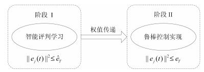 图 2 事件驱动鲁棒自适应评判控制设计过程图Fig. 2 The design procedure of event-triggered robust adaptive critic control
5. 基于学习的自适应$\pmb H_{\bf\infty}$控制设计
如前文所述, 未知参数和外部扰动的广泛存在, 使得设计具有鲁棒特性的控制器变得非常重要.经典的$H_{\infty}$控制针对包含外部扰动和不确定项的动态系统, 构建考虑最坏情形的控制律.根据极大极小最优性原理, $H_{\infty}$控制问题通常被描述为二人零和微分博弈.为了得到在最坏情况下使得代价函数最小化的控制器, 需要寻找对应于Hamilton-Jacobi-Isaacs (HJI)方程的Nash均衡解.然而, 对于一般的非线性系统, 获得HJI方程的解析解是不容易的, 这如同求解非线性最优控制问题HJB方程时遇到的困难.近些年来, ADP思想已被广泛应用于求解$H_{\infty}$控制问题.与自适应最优调节设计类似, 这里称作自适应$H_{\infty}$控制设计, 如文献[91-96]和其中的参考文献.
考虑一类含有外部扰动的连续时间非线性系统
$$ \dot{x}(t)=f(x(t))+g(x(t))u(t)+h(x(t))v(t) $$ (43a) $$ \zeta(t)=y(x(t)) $$ (43b) 其中, $v(t)\in {\bf R}^q$是满足$v(t) \in \mathcal{L}_{2}[0, \infty)$的扰动向量, $\zeta(t)=y(x(t))\in {\bf R}^p$是目标输出, 并且$h(\cdot)$是可微的.
在非线性$H_{\infty}$控制设计中, 通常需要找到一个反馈控制律$u(x)$, 使得闭环系统渐近稳定且具有不大于$\varrho$的$\mathcal{L}_{2}$-增益, 即
$$ \begin{align}\label{Eq36001} \int_{0}^{\infty} \big[\|y(x(\tau))\|^{2}+& u^{\rm T}(\tau)Ru(\tau)\big]\text{d}\tau \leq \nonumber\\& \varrho^{2}\int_{0}^{\infty}v^{\rm T}(\tau)Pv(\tau)\text{d}\tau \end{align} $$ (44) 其中, $\|y(x(t))\|^{2}=x^{\rm T}(t)Qx(t)$, $Q$, $R$, $P$是具有合适维数的对称正定有界矩阵.值得一提的是, $H_{\infty}$控制问题的解是零和博弈理论的鞍点并由一对控制律$(u^{*}, v^{*})$表示, 其中, $u^{*}$和$v^{*}$分别称为最优控制律和最坏情况下的扰动函数.
$$ \begin{align}U(x, u, v)= x^{\rm T}Qx+u^{\rm T}Ru-\varrho^{2}v^{\rm T}Pv\end{align} $$ (45) 并且定义代价函数为
$$ \begin{align} \label{Eq003} J(x(t), u, v)=\int_{t}^{\infty}U(x(\tau), u(\tau), v(\tau))\text{d}\tau \end{align} $$ (46) 我们的目标是找到鞍点解$(u^{*}, v^{*})$, 使得Nash条件
$$ \begin{align} J^{*}(x_{0}) = \min\limits_{u}\max\limits_{v}J(x_{0}, u, v) = \max\limits_{v}\min\limits_{u}J(x_{0}, u, v) \end{align} $$ (47) 成立, 其中, $J^{*}(x_{0})$代表最优代价.对于容许控制$u \in \mathcal{A}(\Omega)$, 如果相关的代价函数(46)是连续可微的, 那么非线性Lyapunov方程为
$$ \begin{align} %\label{Eq005} 0 = U(x, u, v)+(\nabla J(x))^{\rm T}(f+gu+hv) \end{align} $$ (48) 其中, $J(0)=0$.定义被控系统的Hamiltonian为
$$ \begin{align} H(x, &\ u, v, \nabla J(x))= U(x, u, v)+\nonumber\\&\ (\nabla J(x))^{\rm T} (f+gu+hv) \end{align} $$ (49) 利用文献[95]中的结论, 最优控制律和最坏情形的扰动函数分别为
$$ u^{*}(x)=-\frac{1}{2}R^{-1}g^{\rm T}(x) \nabla J^{*}(x) $$ (50a) $$ v^{*}(x)=\frac{1}{2\varrho^{2}}P^{-1}h^{\rm T}(x) \nabla J^{*}(x) $$ (50b) 于是, 此类问题的HJI方程为下面的形式:
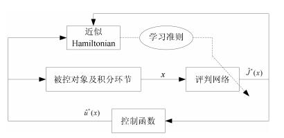
$$ \begin{align} \label{Eq010} 0= & U(x, u^{*}, v^{*})+(\nabla J^{*}(x))^{\rm T} (f+gu^{*}+hv^{*})=\nonumber\\ &H(x, u^{*}, v^{*}, \nabla J^{*}(x)) \end{align} $$ (51) 其中, $J^{*}(0)=0$.利用自适应评判进行$H_{\infty}$控制设计的核心就是构建并训练评判网络, 以近似求解非线性的HJI方程(51).最近, 在事件驱动机制下的自适应$H_{\infty}$控制设计也得到了人们的关注[97-99], 基本的设计框图如图 3所示, 其中的主要组件包括被控对象及积分环节, 评判神经网络, 通信网络媒介, 采样设备组件, 以及零阶保持组件.图 3中的符号$\hat{x}_{j}$是通过网络媒介并由采样设备处理后的事件驱动状态向量, $\hat{J}(\hat{x}_{j})$是评判网络的输出量, $\mu(\hat{x}_{j})$和$v(x)$分别是控制函数和扰动函数输出, 与近似Hamiltonian相关的$e_c$是训练评判网络的基本误差量.值得关注的是, 文献[97]提出基于更新准则的评判网络学习机制, 即
$$ \begin{align} \label{Eq0223}\dot{\hat{\omega}}_{c}=&-\alpha_{c}\frac{\phi}{(1+\phi^{\rm T}\phi)^{2}}e_{c}+\frac{1}{2}\alpha_{s}\bigg[\nabla \sigma_{c}(\hat{x}_{j})g(\hat{x}_{j})\times \nonumber\\&\ g^{\rm T}(x)-\frac{1}{\varrho^{2}}\nabla \sigma_{c}(x)h(x)h^{\rm T}(x)\bigg]\nabla J_{s}(x) \end{align} $$ (52)  图 3 事件驱动自适应$H_{\infty}$控制结构图Fig. 3 Structure of event-triggered adaptive $H_{\infty}$ control
这样, 在基本学习率$\alpha_{c}$和附加调整因子$\alpha_{s}>0$的共同作用下, 控制设计者可以根据实际情况建立更加有效的控制器, 而减缓初始条件限制更具实用意义.
考虑到不确定因素和外部扰动的广泛存在, 利用ADP这一智能学习技术, 构建鲁棒自适应评判系统, 实现复杂非线性系统的自学习鲁棒控制与自适应$H_{\infty}$控制, 具有重要的理论与实际意义.鲁棒自适应评判控制理论与方法, 仍然是相关领域的研究热点, 更多富有意义的成果将不断涌现.
6. 总结与展望
由于在解决复杂系统智能控制和决策问题方面的优势, 基于智能学习的自适应评判控制设计已经有许多成功的应用.复杂的工业系统, 如电力与能源系统[23, 31, 64-68, 85, 100-105], 机械系统[13-14, 26, 58, 60, 66, 78, 106], 智能交通系统[107-108]是最常见的应用领域.文献[103]提出针对频率控制问题的自适应评判设计方法, 以实现智能电网的频率稳定.文献[105]建立一种基于天气分类的新型电能自适应优化方法, 能够有效管理电能流动, 平衡电网负载, 而且实施错峰用电可以减少居民的电费支出.文献[106]针对运载工业中常用的吊车系统, 设计有效的自适应优化控制方案.文献[107]和[108]则分别给出ADP方法在交通信号控制和车联网技术方面的研究成果, 为建立智能交通系统提供了一定的方法保障.除此之外, 很多学者仍然在开展大量具有实际应用背景的研究工作, 以期取得更加显著的经济和社会效益.
尽管在自适应评判控制及鲁棒镇定设计方面, 已经有很多优秀的成果, 但是仍然需要进一步研究策略学习算法的收敛性和被控系统的稳定性以及最优性与鲁棒性等各种基础问题.例如, 克服神经网络逼近的缺点, 实现全局最优镇定就值得进一步研究.如何进一步降低策略学习算法对于初始条件的依赖也是很有意义的主题.关于离散时间系统的鲁棒自适应评判控制, 也期待有更多的研究成果出现, 以完善复杂动态系统的智能化设计体系.结合抽象动态规划[109]理论进行自适应评判设计也是一个有趣的方向.另外, 强化学习系统的一个重要特性是可以高效利用数据资源.如何更加有效地利用数据信息来建立更为先进的数据驱动控制方法是非常关键的.在这一主题上, 迭代神经动态规划算法[20-21], 积分强化学习技术[32], 计算控制方法[43]和并行学习算法[98]都是有意义的尝试.特别地, 将深度学习与ADP及强化学习相结合产生的深度强化学习, 不仅已经在AlphaGo Zero [6]中取得了重大成功, 还将有助于我们构建更多的智能系统并实现更高水平的类脑智能.深度强化学习能够直接基于图像的输入来输出控制信号, 同时具备深度学习的感知能力和强化学习的决策优点[2].这种机制使得人工智能与人类的思维模式非常接近, 因此, 迫切需要深入地研究其在自适应评判设计中的应用.同时, 在考虑不确定因素和鲁棒性能的情况下, 如何得到含有高效数据驱动和智能学习组件的鲁棒最优控制策略, 也需要进一步研究.此外, 对于网络化系统, 充分考虑通信因素是很有必要的.需要深入讨论事件驱动机制的实施办法, 不局限于针对控制函数.如何将基于数据的方法与事件驱动机制相结合, 进行混合数据-事件驱动控制也是很有意义的.这样不仅可以高效利用数据资源, 而且可以显著降低通信负担, 实现有效的混合驱动控制, 进而可以推广研究混合驱动的鲁棒轨迹跟踪和$H_{\infty}$控制设计.最后, 需要将现有的结果扩展到多智能体系统, 以实现网络化系统的分布式协同优化.所以, 在不确定环境下, 基于自适应评判的分布式设计与分散控制设计是处理复杂系统智能控制与管理问题的另一个很有发展前景的方向.
近年来, 脑科学与类脑智能的研究已经引起各国学者的极大兴趣.越来越多的证据表明, 最优性在理解大脑智能的研究中具有重要作用.考虑以在线方式实现对具有不确定性和未知动态的复杂系统进行最优决策和智能控制这一宗旨, ADP可以为智能系统和类脑智能研究做出相当大的贡献.正如其创始人Werbos博士指出的, ADP很可能是实现真正意义类脑智能的关键方法[110].因此, 为降低计算量和通信负担的近似动态规划解决方案, 包括保证稳定性、收敛性、最优性和鲁棒性的研究仍然需要大批学者的努力, 其中, 基于智能学习的鲁棒自适应评判控制设计也一定能够取得更大的进展.
-
图 2 事件驱动鲁棒自适应评判控制设计过程图
Fig. 2 The design procedure of event-triggered robust adaptive critic control
-
[1] Silver D, Huang A, Maddison C J, Guez A, Sifre L, van den Driessche G, et al. Mastering the game of Go with deep neural networks and tree search. Nature, 2016, 529(7587):484-489 doi: 10.1038/nature16961 [2] LeCun Y, Bengio Y, Hinton G. Deep learning. Nature, 2015, 521(7553):436-444 doi: 10.1038/nature14539 [3] Schmidhuber J. Deep learning in neural networks:an overview. Neural Networks, 2015, 61:85-117 doi: 10.1016/j.neunet.2014.09.003 [4] Haykin S. Neural Networks: A Comprehensive Foundation (Second edition). Upper Saddle River, NJ: Prentice-Hall, 1999. [5] Sutton R S, Barto A G. Reinforcement Learning:An Introduction. Cambridge, MA:MIT Press, 1998. [6] Silver D, Schrittwieser J, Simonyan K, Antonoglou I, Huang A, Guez A, et al. Mastering the game of Go without human knowledge. Nature, 2017, 550:354-359 doi: 10.1038/nature24270 [7] Bellman R E. Dynamic Programming. Princeton, NJ:Princeton University Press, 1957. [8] Lewis F L, Vrabie D, Syrmos V L. Optimal Control (Third edition). New York:Wiley, 2012. [9] Werbos P J. Beyond Regression: New Tools for Prediction and Analysis in the Behavioral Sciences[Ph. D. dissertation], Harvard University, Cambridge, MA, 1974 [10] Werbos P J. Advanced forecasting methods for global crisis warning and models of intelligence. General Systems Yearbook, 1977, 22(6):25-38 [11] Werbos P J. Approximate dynamic programming for realtime control and neural modeling. Handbook of Intelligent Control: Neural, Fuzzy, and Adaptive Approaches. New York, NY: Van Nostrand Reinhold, 1992. [12] Prokhorov D V, Wunsch D C. Adaptive critic designs. IEEE Transactions on Neural Networks, 1997, 8(5):997-1007 doi: 10.1109/72.623201 [13] Murray J J, Cox C J, Lendaris G G, Saeks R. Adaptive dynamic programming. IEEE Transactions on Systems, Man, and Cybernetics, Part C:Applications and Reviews, 2002, 32(2):140-153 doi: 10.1109/TSMCC.2002.801727 [14] Si J, Wang Y T. Online learning control by association and reinforcement. IEEE Transactions on Neural Networks, 2001, 12(2):264-276 doi: 10.1109/72.914523 [15] Saridis G N, Wang F Y. Suboptimal control of nonlinear stochastic systems. Control Theory and Advanced Technology, 1994, 10(4):847-871 [16] Beard R W, Saridis G N, Wen J T. Galerkin approximations of the generalized Hamilton-Jacobi-Bellman equation. Automatica, 1997, 33(12):2159-2177 doi: 10.1016/S0005-1098(97)00128-3 [17] Abu-Khalaf M, Lewis F L. Nearly optimal control laws for nonlinear systems with saturating actuators using a neural network HJB approach. Automatica, 2005, 41(5):779-791 doi: 10.1016/j.automatica.2004.11.034 [18] Wang D, Liu D R, Wei Q L, Zhao D B, Jin N. Optimal control of unknown nona-ne nonlinear discrete-time systems based on adaptive dynamic programming. Automatica, 2012, 48(8):1825-1832 doi: 10.1016/j.automatica.2012.05.049 [19] Xu B, Yang C G, Shi Z K. Reinforcement learning output feedback NN control using deterministic learning technique. IEEE Transactions on Neural Networks and Learning Systems, 2014, 25(3):635-641 doi: 10.1109/TNNLS.2013.2292704 [20] 王鼎, 穆朝絮, 刘德荣.基于迭代神经动态规划的数据驱动非线性近似最优调节.自动化学报, 2017, 43(3):366-375 http://www.aas.net.cn/CN/abstract/abstract19015.shtmlWang Ding, Mu Chao-Xu, Liu De-Rong. Data-driven nonlinear near-optimal regulation based on iterative neural dynamic programming. Acta Automatica Sinica, 2017, 43(3):366-375 http://www.aas.net.cn/CN/abstract/abstract19015.shtml [21] Mu C X, Wang D, He H B. Novel iterative neural dynamic programming for data-based approximate optimal control design. Automatica, 2017, 81:240-252 doi: 10.1016/j.automatica.2017.03.022 [22] Vamvoudakis K G, Lewis F L. Online actor-critic algorithm to solve the continuous-time inflnite horizon optimal control problem. Automatica, 2010, 46(5):878-888 doi: 10.1016/j.automatica.2010.02.018 [23] Vamvoudakis K G, Miranda M F, Hespanha J P. Asymptotically stable adaptive-optimal control algorithm with saturating actuators and relaxed persistence of excitation. IEEE Transactions on Neural Networks and Learning Systems, 2016, 27(11):2386-2398 doi: 10.1109/TNNLS.2015.2487972 [24] Bhasin S, Kamalapurkar R, Johnson M, Vamvoudakis K G, Lewis F L, Dixon W E. A novel actor-critic-identifler architecture for approximate optimal control of uncertain nonlinear systems. Automatica, 2013, 49(1):82-92 doi: 10.1016/j.automatica.2012.09.019 [25] Modares H, Lewis F L. Optimal tracking control of nonlinear partially-unknown constrained-input systems using integral reinforcement learning. Automatica, 2014, 50(7):1780-1792 doi: 10.1016/j.automatica.2014.05.011 [26] Nodland D, Zargarzadeh H, Jagannathan S. Neural network-based optimal adaptive output feedback control of a helicopter UAV. IEEE Transactions on Neural Networks and Learning Systems, 2013, 24(7):1061-1073 doi: 10.1109/TNNLS.2013.2251747 [27] Lv Y F, Na J, Yang Q M, Wu X, Guo Y. Online adaptive optimal control for continuous-time nonlinear systems with completely unknown dynamics. International Journal of Control, 2016, 89(1):99-112 doi: 10.1080/00207179.2015.1060362 [28] Vrabie D, Lewis F. Neural network approach to continuous-time direct adaptive optimal control for partially unknown nonlinear systems. Neural Networks, 2009, 22(3):237-246 doi: 10.1016/j.neunet.2009.03.008 [29] Zhang H G, Cui L L, Zhang X, Luo Y H. Data-driven robust approximate optimal tracking control for unknown general nonlinear systems using adaptive dynamic programming method. IEEE Transactions on Neural Networks, 2011, 22(12):2226-2236 doi: 10.1109/TNN.2011.2168538 [30] Jiang Y, Jiang Z P. Global adaptive dynamic programming for continuous-time nonlinear systems. IEEE Transactions on Automatic Control, 2015, 60(11):2917-2929 doi: 10.1109/TAC.2015.2414811 [31] Bian T, Jiang Z P. Value iteration and adaptive dynamic programming for data-driven adaptive optimal control design. Automatica, 2016, 71:348-360 doi: 10.1016/j.automatica.2016.05.003 [32] Lee J Y, Park J B, Choi Y H. Integral reinforcement learning for continuous-time input-a-ne nonlinear systems with simultaneous invariant explorations. IEEE Transactions on Neural Networks and Learning Systems, 2015, 26(5):916-932 doi: 10.1109/TNNLS.2014.2328590 [33] Ha M M, Wang D, Liu D R. Event-triggered adaptive critic control design for discrete-time constrained nonlinear systems. IEEE Transactions on Systems, Man and Cybernetics:Systems, 2019, DOI: 10.1109/TSMC.2018.2868510 [34] Wang F Y, Zhang H G, Liu D R. Adaptive dynamic programming:an introduction. IEEE Computational Intelligence Magazine, 2009, 4(2):39-47 doi: 10.1109/MCI.2009.932261 [35] Lewis F L, Liu D R. Reinforcement Learning and Approximate Dynamic Programming for Feedback Control. Hoboken, NJ: John Wiley & Sons, Inc., 2012. [36] Zhang H G, Liu D R, Luo Y H, Wang D. Adaptive Dynamic Programming for Control: Algorithms and Stability. London, UK: Springer-Verlag, 2013. [37] 张化光, 张欣, 罗艳红, 杨珺.自适应动态规划综述.自动化学报, 2013, 39(4):303-311 http://www.aas.net.cn/CN/abstract/abstract17916.shtmlZhang Hua-Guang, Zhang Xin, Luo Yan-Hong, Yang Jun. An overview of research on adaptive dynamic programming. Acta Automatica Sinica, 2013, 39(4):303-311 http://www.aas.net.cn/CN/abstract/abstract17916.shtml [38] 刘德荣, 李宏亮, 王鼎.基于数据的自学习优化控制:研究进展与展望.自动化学报, 2013, 39(11):1858-1870 http://www.aas.net.cn/CN/abstract/abstract18225.shtmlLiu De-Rong, Li Hong-Liang, Wang Ding. Data-based selflearning optimal control:research progress and prospects. Acta Automatica Sinica, 2013, 39(11):1858-1870 http://www.aas.net.cn/CN/abstract/abstract18225.shtml [39] Wang D, He H B, Liu D R. Adaptive critic nonlinear robust control:a survey. IEEE Transactions on Cybernetics, 2017, 47(10):3429-3451 doi: 10.1109/TCYB.2017.2712188 [40] Wang D, Mu C X. Adaptive Critic Control with Robust Stabilization for Uncertain Nonlinear Systems. Singapore: Springer Singapore, 2019. [41] Liu D R, Wei Q L, Wang D, Yang X, Li H L. Adaptive Dynamic Programming with Applications in Optimal Control. Switzerland: Springer, 2017. [42] Jiang Y, Jiang Z P. Robust Adaptive Dynamic Programming. Hoboken, NJ:Wiley-IEEE Press, 2017. [43] 王飞跃.平行控制:数据驱动的计算控制方法.自动化学报, 2013, 39(4):293-302 http://www.aas.net.cn/CN/abstract/abstract17915.shtmlWang Fei-Yue. Parallel control:a method for data-driven and computational control. Acta Automatica Sinica, 2013, 39(4):293-302 http://www.aas.net.cn/CN/abstract/abstract17915.shtml [44] Hou Z S, Wang Z. From model-based control to datadriven control:Survey, classiflcation and perspective. Information Sciences, 2013, 235:3-35 doi: 10.1016/j.ins.2012.07.014 [45] Lavretsky E, Wise K A. Robust and Adaptive Control: with Aerospace Applications. London, UK: SpringerVerlag, 2013. [46] Krstic M, Kanellakopoulos I, Kokotovic P V. Nonlinear and Adaptive Control Design. New York, NY: John Wiley & Sons, 1995. [47] Lewis F L, Jagannathan S, Yesildirek A. Neural Network Control of Robot Manipulators and Non-linear Systems. London: Taylor & Francis, 1999. [48] Corless M, Leitmann G. Continuous state feedback guaranteeing uniform ultimate boundedness for uncertain dynamic systems. IEEE Transactions on Automatic Control, 1981, 26(5):1139-1144 doi: 10.1109/TAC.1981.1102785 [49] Lin F. Robust Control Design: An Optimal Control Approach. Chichester: John Wiley & Sons, 2007. [50] Lin F, Brand R D, Sun J. Robust control of nonlinear systems:Compensating for uncertainty. International Journal of Control, 1992, 56(6):1453-1459 doi: 10.1080/00207179208934374 [51] Adhyaru D M, Kar I N, Gopal M. Fixed flnal time optimal control approach for bounded robust controller design using Hamilton-Jacobi-Bellman solution. IET Control Theory & Applications, 2009, 3(9):1183-1195 [52] Adhyaru D M, Kar I N, Gopal M. Bounded robust control of nonlinear systems using neural network-based HJB solution. Neural Computing & Applications, 2011, 20(1):91-103 [53] Wang D, Liu D R, Li H L. Policy iteration algorithm for online design of robust control for a class of continuoustime nonlinear systems. IEEE Transactions on Automation Science and Engineering, 2014, 11(2):627-632 doi: 10.1109/TASE.2013.2296206 [54] Wang D, Liu D R, Li H L, Ma H W. Neural-network-based robust optimal control design for a class of uncertain nonlinear systems via adaptive dynamic programming. Information Sciences, 2014, 282:167-179 doi: 10.1016/j.ins.2014.05.050 [55] Wang D, Liu D R, Zhang Q C, Zhao D B. Data-based adaptive critic designs for nonlinear robust optimal control with uncertain dynamics. IEEE Transactions on Systems, Man, and Cybernetics:Systems, 2016, 46(11):1544-1555 doi: 10.1109/TSMC.2015.2492941 [56] Liu D R, Yang X, Wang D, Wei Q L. Reinforcementlearning-based robust controller design for continuoustime uncertain nonlinear systems subject to input constraints. IEEE Transactions on Cybernetics, 2015, 45(7):1372-1385 doi: 10.1109/TCYB.2015.2417170 [57] Wang D, Liu D R, Li H L, Luo B, Ma H W. An approximate optimal control approach for robust stabilization of a class of discrete-time nonlinear systems with uncertainties. IEEE Transactions on Systems, Man, and Cybernetics:Systems, 2016, 46(5):713-717 doi: 10.1109/TSMC.2015.2466191 [58] Wang D. Adaptation-oriented near-optimal control and robust synthesis of an overhead crane system. In: Proceedings of the 2017 International Conference on Neural Information Processing. Guangzhou, China: Springer, 2017. 42-50 [59] Zhong X N, He H B, Prokhorov D V. Robust controller design of continuous-time nonlinear system using neural network. In: Proceedings of the 2013 International Joint Conference on Neural Networks. Dallas, TX, USA: IEEE, 2013. 1-8 [60] Sun J L, Liu C S, Ye Q. Robust difierential game guidance laws design for uncertain interceptor-target engagement via adaptive dynamic programming. International Journal of Control, 2017, 90(5):990-1004 doi: 10.1080/00207179.2016.1192687 [61] Wang D, Li C, Liu D R, Mu C X. Data-based robust optimal control of continuous-time a-ne nonlinear systems with matched uncertainties. Information Sciences, 2016, 366:121-133 doi: 10.1016/j.ins.2016.05.034 [62] Yang X, Liu D R, Luo B, Li C. Data-based robust adaptive control for a class of unknown nonlinear constrained-input systems via integral reinforcement learning. Information Sciences, 2016, 369:731-747 doi: 10.1016/j.ins.2016.07.051 [63] Fan Q Y, Yang G H. Adaptive actor-critic design-based integral sliding-mode control for partially unknown nonlinear systems with input disturbances. IEEE Transactions on Neural Networks and Learning Systems, 2016, 27(1):165-177 doi: 10.1109/TNNLS.2015.2472974 [64] Jiang Y, Jiang Z P. Robust adaptive dynamic programming for large-scale systems with an application to multimachine power systems. IEEE Transactions on Circuits and Systems Ⅱ:Express Briefs, 2012, 59(10):693-697 doi: 10.1109/TCSII.2012.2213353 [65] Jiang Z P, Jiang Y. Robust adaptive dynamic programming for linear and nonlinear systems:an overview. European Journal of Control, 2013, 19(5):417-425 doi: 10.1016/j.ejcon.2013.05.017 [66] Jiang Y, Jiang Z P. Robust adaptive dynamic programming and feedback stabilization of nonlinear systems. IEEE Transactions on Neural Networks and Learning Systems, 2014, 25(5):882-893 doi: 10.1109/TNNLS.2013.2294968 [67] Bian T, Jiang Y, Jiang Z P. Decentralized adaptive optimal control of large-scale systems with application to power systems. IEEE Transactions on Industrial Electronics, 2015, 62(4):2439-2447 doi: 10.1109/TIE.2014.2345343 [68] Gao W N, Jiang Y, Jiang Z P, Chai T Y. Output-feedback adaptive optimal control of interconnected systems based on robust adaptive dynamic programming. Automatica, 2016, 72:37-45 doi: 10.1016/j.automatica.2016.05.008 [69] Dierks T, Jagannathan S. Optimal control of a-ne nonlinear continuous-time systems. In: Proceedings of the 2010 American Control Conference. Baltimore, MD, USA: IEEE, 2010. 1568-1573 [70] Zhang H G, Cui L L, Luo Y H. Near-optimal control for nonzero-sum difierential games of continuous-time nonlinear systems using single-network ADP. IEEE Transactions on Cybernetics, 2013, 43(1):206-216 doi: 10.1109/TSMCB.2012.2203336 [71] Yang X, Liu D R, Ma H W, Xu Y C. Online approximate solution of HJI equation for unknown constrained-input nonlinear continuous-time systems. Information Sciences, 2016, 328:435-454 doi: 10.1016/j.ins.2015.09.001 [72] Wang D, Mu C. Developing nonlinear adaptive optimal regulators through an improved neural learning mechanism. Science China Information Sciences, 2017, 60(5):058201 doi: 10.1007/s11432-016-9022-1 [73] Wang D, Mu C X. A novel neural optimal control framework with nonlinear dynamics:Closed-loop stability and simulation veriflcation. Neurocomputing, 2017, 266:353-360 doi: 10.1016/j.neucom.2017.05.051 [74] Wang D, Liu D R, Mu C X, Zhang Y. Neural network learning and robust stabilization of nonlinear systems with dynamic uncertainties. IEEE Transactions on Neural Networks and Learning Systems, 2018, 29(4):1342-1351 doi: 10.1109/TNNLS.2017.2749641 [75] Yang X, He H B. Self-learning robust optimal control for continuous-time nonlinear systems with mismatched disturbances. Neural Networks, 2018, 99:19-30 doi: 10.1016/j.neunet.2017.11.022 [76] Jiang Z P, Teel A R, Praly L. Small-gain theorem for ISS systems and applications. Mathematics of Control, Signals and Systems, 1994, 7(2):95-120 doi: 10.1007/BF01211469 [77] Mu C X, Sun C Y, Wang D, Song A G. Adaptive tracking control for a class of continuous-time uncertain nonlinear systems using the approximate solution of HJB equation. Neurocomputing, 2017, 260:432-442 doi: 10.1016/j.neucom.2017.04.043 [78] Wang D, Mu C X. Adaptive-critic-based robust trajectory tracking of uncertain dynamics and its application to a spring-mass-damper system. IEEE Transactions on Industrial Electronics, 2018, 65(1):654-663 doi: 10.1109/TIE.2017.2722424 [79] Wang D, Liu D R, Zhang Y, Li H Y. Neural network robust tracking control with adaptive critic framework for uncertain nonlinear systems. Neural Networks, 2018, 97:11-18 doi: 10.1016/j.neunet.2017.09.005 [80] Tabuada P. Event-triggered real-time scheduling of stabilizing control tasks. IEEE Transactions on Automatic Control, 2007, 52(9):1680-1685 doi: 10.1109/TAC.2007.904277 [81] Tallapragada P, Chopra N. On event triggered tracking for nonlinear systems. IEEE Transactions on Automatic Control, 2013, 58(9):2343-2348 doi: 10.1109/TAC.2013.2251794 [82] Vamvoudakis K G. Event-triggered optimal adaptive control algorithm for continuous-time nonlinear systems. IEEE/CAA Journal of Automatica Sinica, 2014, 1(3):282-293 doi: 10.1109/JAS.2014.7004686 [83] Sahoo A, Xu H, Jagannathan S. Neural networkbased event-triggered state feedback control of nonlinear continuous-time systems. IEEE Transactions on Neural Networks and Learning Systems, 2016, 27(3):497-509 doi: 10.1109/TNNLS.2015.2416259 [84] Zhong X N, He H B. An event-triggered ADP control approach for continuous-time system with unknown internal states. IEEE Transactions on Cybernetics, 2017, 47(3):683-694 doi: 10.1109/TCYB.2016.2523878 [85] Dong L, Tang Y F, He H B, Sun C Y. An event-triggered approach for load frequency control with supplementary ADP. IEEE Transactions on Power Systems, 2017, 32(1):581-589 doi: 10.1109/TPWRS.2016.2537984 [86] Zhu Y H, Zhao D B, He H B, Ji J H. Event-triggered optimal control for partially unknown constrained-input systems via adaptive dynamic programming. IEEE Transactions on Industrial Electronics, 2017, 64(5):4101-4109 doi: 10.1109/TIE.2016.2597763 [87] Wang D, Mu C X, He H B, Liu D R. Adaptive-critic-based event-driven nonlinear robust state feedback. In: Proceedings of the IEEE 55th Conference on Decision and Control. Las Vegas, NV, USA: IEEE, 2016. 5813-5818 [88] Wang D, Mu C X, He H B, Liu D R. Event-driven adaptive robust control of nonlinear systems with uncertainties through NDP strategy. IEEE Transactions on Systems, Man, and Cybernetics:Systems, 2017, 47(7):1358-1370 doi: 10.1109/TSMC.2016.2592682 [89] Wang D, Liu D R. Neural robust stabilization via eventtriggering mechanism and adaptive learning technique. Neural Networks, 2018, 102:27-35 doi: 10.1016/j.neunet.2018.02.007 [90] Zhang Q C, Zhao D B, Wang D. Event-based robust control for uncertain nonlinear systems using adaptive dynamic programming. IEEE Transactions on Neural Networks and Learning Systems, 2018, 29(1):37-50 doi: 10.1109/TNNLS.2016.2614002 [91] Abu-Khalaf M, Lewis F L, Huang J. Policy iterations on the Hamilton-Jacobi-Isaacs equation for H∞ state feedback control with input saturation. IEEE Transactions on Automatic Control, 2006, 51(12):1989-1995 doi: 10.1109/TAC.2006.884959 [92] Vamvoudakis K G, Lewis F L. Online solution of nonlinear two-player zero-sum games using synchronous policy iteration. International Journal of Robust and Nonlinear Control, 2012, 22(13):1460-1483 doi: 10.1002/rnc.v22.13 [93] Modares H, Lewis F L, Sistani M B N. Online solution of nonquadratic two-player zero-sum games arising in the H∞ control of constrained input systems. International Journal of Adaptive Control and Signal Processing, 2014, 28(3-5):232-254 doi: 10.1002/acs.v28.3-5 [94] Luo B, Wu H N, Huang T W. Ofi-policy reinforcement learning for H∞ control design. IEEE Transactions on Cybernetics, 2015, 45(1):65-76 doi: 10.1109/TCYB.2014.2319577 [95] Zhang H G, Qin C B, Jiang B, Luo Y H. Online adaptive policy learning algorithm for H∞ state feedback control of unknown a-ne nonlinear discrete-time systems. IEEE Transactions on Cybernetics, 2014, 44(12):2706-2718 doi: 10.1109/TCYB.2014.2313915 [96] Song R Z, Lewis F L, Wei Q L, Zhang H G. Ofi-policy actor-critic structure for optimal control of unknown systems with disturbances. IEEE Transactions on Cybernetics, 2016, 46(5):1041-1050 doi: 10.1109/TCYB.2015.2421338 [97] Wang D, He H B, Liu D R. Improving the critic learning for event-based nonlinear H∞ control design. IEEE Transactions on Cybernetics, 2017, 47(10):3417-3428 doi: 10.1109/TCYB.2017.2653800 [98] Zhang Q C, Zhao D B, Zhu Y H. Event-triggered H∞ control for continuous-time nonlinear system via concurrent learning. IEEE Transactions on Systems, Man, and Cybernetics:Systems, 2017, 47(7):1071-1081 doi: 10.1109/TSMC.2016.2531680 [99] Mu C X, Wang D, Sun C Y, Zong Q. Robust adaptive critic control design with network-based event-triggered formulation. Nonlinear Dynamics, 2017, 90(3):2023-2035 doi: 10.1007/s11071-017-3778-5 [100] Werbos P J. Computational intelligence for the smart gridhistory, challenges, and opportunities. IEEE Computational Intelligence Magazine, 2011, 6(3):14-21 doi: 10.1109/MCI.2011.941587 [101] Tang Y F, He H B, Wen J Y, Liu J. Power system stability control for a wind farm based on adaptive dynamic programming. IEEE Transactions on Smart Grid, 2015, 6(1):166-177 doi: 10.1109/TSG.2014.2346740 [102] Wang D, He H B, Mu C X, Liu D R. Intelligent critic control with disturbance attenuation for a-ne dynamics including an application to a microgrid system. IEEE Transactions on Industrial Electronics, 2017, 64(6):4935-4944 doi: 10.1109/TIE.2017.2674633 [103] Wang D, He H B, Zhong X N, Liu D R. Event-driven nonlinear discounted optimal regulation involving a power system application. IEEE Transactions on Industrial Electronics, 2017, 64(10):8177-8186 doi: 10.1109/TIE.2017.2698377 [104] Wei Q L, Lewis F L, Shi G, Song R Z. Error-tolerant iterative adaptive dynamic programming for optimal renewable home energy scheduling and battery management. IEEE Transactions on Industrial Electronics, 2017, 64(12):9527-9537 doi: 10.1109/TIE.2017.2711499 [105] Liu D R, Xu Y C, Wei Q L, Liu X L. Residential energy scheduling for variable weather solar energy based on adaptive dynamic programming. IEEE/CAA Journal of Automatica Sinica, 2018, 5(1):36-46 doi: 10.1109/JAS.2017.7510739 [106] Wang D, He H B, Liu D R. Intelligent optimal control with critic learning for a nonlinear overhead crane system. IEEE Transactions on Industrial Informatics, 2018, 14(7):2932-2940 doi: 10.1109/TII.2017.2771256 [107] 赵冬斌, 刘德荣, 易建强.基于自适应动态规划的城市交通信号优化控制方法综述.自动化学报, 2009, 35(6):676-681 http://www.aas.net.cn/CN/abstract/abstract13331.shtmlZhao Dong-Bin, Liu De-Rong, Yi Jian-Qiang. An overview on the adaptive dynamic programming based urban city tra-c signal optimal control. Acta Automatica Sinica, 2009, 35(6):676-681 http://www.aas.net.cn/CN/abstract/abstract13331.shtml [108] Gao W N, Jiang Z P, Ozbay K. Data-driven adaptive optimal control of connected vehicles. IEEE Transactions on Intelligent Transportation Systems, 2017, 18(5):1122-1133 doi: 10.1109/TITS.2016.2597279 [109] Bertsekas D P. Value and policy iterations in optimal control and adaptive dynamic programming. IEEE Transactions on Neural Networks and Learning Systems, 2017, 28(3):500-509 doi: 10.1109/TNNLS.2015.2503980 [110] Werbos P J. From ADP to the brain: Foundations, roadmap, challenges and research priorities. In: Proceedings of the 2014 International Joint Conference on Neural Networks. Beijing, China: IEEE, 2014. 107-111 期刊类型引用(15)
1. 时侠圣,任璐,孙长银. 自适应分布式聚合博弈广义纳什均衡算法. 自动化学报. 2024(06): 1210-1220 .  本站查看
本站查看2. 王鼎,胡凌治,赵明明,哈明鸣,乔俊飞. 未知非线性零和博弈最优跟踪的事件触发控制设计. 自动化学报. 2023(01): 91-101 . 本站查看3. 吴健发,王宏伦,王延祥,刘一恒. 无人机反应式扰动流体路径规划. 自动化学报. 2023(02): 272-287 . 本站查看4. 吴清平. 改进的暗通道运动图像盲复原方法. 山东理工大学学报(自然科学版). 2023(05): 68-73 . 百度学术5. 霍煜,王鼎,乔俊飞. 基于单网络评判学习的非线性系统鲁棒跟踪控制. 控制与决策. 2023(11): 3066-3074 . 百度学术6. 李梦花 ,王鼎 ,乔俊飞 . 不对称约束多人非零和博弈的自适应评判控制. 控制理论与应用. 2023(09): 1562-1568 . 百度学术7. 张兴龙,陆阳,李文璋,徐昕. 基于滚动时域强化学习的智能车辆侧向控制算法. 自动化学报. 2023(12): 2481-2492 . 本站查看8. 王鼎. 一类离散动态系统基于事件的迭代神经控制. 工程科学学报. 2022(03): 411-419 . 百度学术9. 王鼎,赵明明,哈明鸣,乔俊飞. 基于折扣广义值迭代的智能最优跟踪及应用验证. 自动化学报. 2022(01): 182-193 . 本站查看10. 石永霞,胡庆雷,邵小东. 角速度受限下航天器姿态机动事件触发控制. 中国科学:信息科学. 2022(03): 506-520 . 百度学术11. 汪雨劼,杜翔宇,刘磊,成忠涛,王永骥. 基于鲁棒自适应动态规划的临近空间飞行器姿态跟踪控制. 战术导弹技术. 2022(02): 75-82 . 百度学术12. 王敏,黄龙旺,杨辰光. 基于事件触发的离散MIMO系统自适应评判容错控制. 自动化学报. 2022(05): 1234-1245 . 本站查看13. 何斌,刘全,张琳琳,时圣苗,陈红名,闫岩. 一种加速时间差分算法收敛的方法. 自动化学报. 2021(07): 1679-1688 . 本站查看14. 吕永峰,田建艳,菅垄,任雪梅. 非线性多输入系统的近似动态规划H_∞控制. 控制理论与应用. 2021(10): 1662-1670 . 百度学术15. 杨勐荷,郑雷. 利用计算机交互技术的网页界面文本视觉优化设计. 现代电子技术. 2020(24): 92-95+101 . 百度学术其他类型引用(18)
-

 下载:
下载:
 下载:
下载:
计量
- 文章访问数: 3083
- HTML全文浏览量: 527
- PDF下载量: 1280
- 被引次数: 33
