

-
摘要: 为解决一类非参数不确定系统在任意初态且输入增益未知情形下的轨迹跟踪问题, 提出准最优误差跟踪学习控制方法.该方法综合准最优控制和迭代学习控制两种技术设计控制器, 在构造期望误差轨迹的基础上, 根据控制Lyapunov函数及Sontag公式给出标称系统的优化控制, 以鲁棒方法和学习方法相结合的策略处理非参数不确定性.闭环系统经过足够次迭代运行后, 经由实现系统误差对期望误差轨迹在整个作业区间上的精确跟踪, 获得系统状态对参考信号在预设的部分作业区间上的精确跟踪.仿真结果表明所设计学习系统在收敛速度方面快于非优化设计.Abstract: This paper presents a suboptimal error-tracking iterative learning control (ILC) scheme to solve the trajectory-tracking problem for a class of nonparametric systems with uncertain input gains in the presence of arbitrary initial states. The ILC controller is developed by integrating ILC with suboptimal control. Firstly, a desired error trajectory is constructed according to the given method, and then Sontag formula is employed for the control design of nominal system, while robust control and learning control are synthetically applied to deal with nonparametric uncertainties. While the closed-loop system operates, as iteration number increases, the controller can render system error to perfectly follow its desired error trajectory over the entire time interval, by which, the system state can precisely track its reference signal in the pre-specified part of above-mentioned interval. Numerical simulations demonstrate that our suboptimal error-track ILC scheme improves convergence performance in comparison with conventional solutions.
-
Key words:
- Suboptimal nonlinear control /
- iterative learning control /
- initial condition problem /
- error-tracking learning control /
- nonparametric systems
1) 本文责任编委 王占山 -
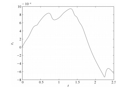
图 5 $e_{1, k}$和$e_{1, k}^*$之差
Fig. 5 The difference between $e_{1, k}$ and $e_{1, k}^*$
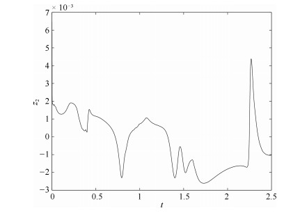
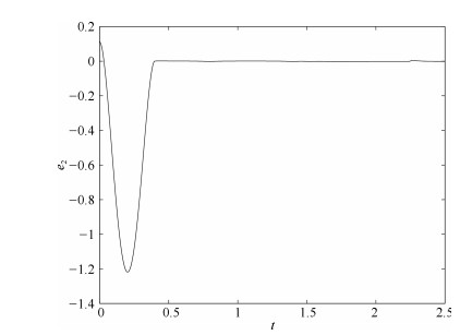
图 6 $e_{2, k}$和$e_{2, k}^*$之差
Fig. 6 The difference between $e_{2, k}$ and $e_{2, k}^*$
-
[1] Xu J X, Tan Y. A composite energy function-based learning control approach for nonlinear systems with time-varying parametric uncertainties. IEEE Transactions on Automatic Control, 2002, 47(11): 1940-1945 doi: 10.1109/TAC.2002.804460 [2] Tayebi A, Chien C J. A unified adaptive iterative learning control framework for uncertain nonlinear systems. IEEE Transactions on Automatic Control, 2007, 52(10): 1907-1913 doi: 10.1109/TAC.2007.906215 [3] Hu T J, Low K H, Shen L C, Xu X. Effective phase tracking for bioinspired undulations of robotic fish models: a learning control approach. IEEE/ASME Transactions on Mechatronics, 2014, 19(1): 191-200 [4] Huang D Q, Xu J X, Venkataramanan V, The Cat Tuong Huynh. High-performance tracking of piezoelectric positioning stage using current-cycle iterative learning control with gain scheduling. IEEE Transactions on Industrial Electronics, 2014, 61(2): 1085-1098 doi: 10.1109/TIE.2013.2253071 [5] Shen D, Wang Y Q. Survey on stochastic iterative learning control. Journal of Process Control, 2014, 24(12): 64-77 doi: 10.1016/j.jprocont.2014.04.013 [6] 张玉东, 方勇纯.一类输出饱和系统的学习控制算法研究.自动化学报, 2011, 37(1): 92-98 doi: 10.3969/j.issn.1003-8930.2011.01.016Zhang Yu-Dong, Fang Yong-Chun. Learning control for systems with saturated output. Acta Automatica Sinica, 2011, 37(1): 92-98 doi: 10.3969/j.issn.1003-8930.2011.01.016 [7] 张黎, 刘山.非最小相位系统的基函数型自适应迭代学习控制.自动化学报, 2014, 40(12): 2716-2725 doi: 10.3724/SP.J.1004.2014.02716Zhang Li, Liu Shan. Basis function based adaptive iterative learning control for non-minimum phase systems. Acta Automatica Sinica, 2014, 40(12): 2716-2725 doi: 10.3724/SP.J.1004.2014.02716 [8] Dai X S, Tian S P, Peng Y J, Luo W G. Closed-loop P-type iterative learning control of uncertain linear distributed parameter systems. IEEE/CAA Journal of Automatica Sinica, 2014, 1(3): 267-273 [9] 卜旭辉, 侯忠生, 余发山, 付子义.基于迭代学习的农业车辆路径跟踪控制.自动化学报, 2014, 40(2): 368-372 doi: 10.3724/SP.J.1004.2014.00368Bu Xu-Hui, Hou Zhong-Sheng, Yu Fa-Shan, Fu Zi-Yi. Iterative learning control for trajectory tracking of farm vehicles. Acta Automatica Sinica, 2014, 40(2): 368-372 doi: 10.3724/SP.J.1004.2014.00368 [10] 李岩, 陈阳泉, 安孝晟.分数阶迭代学习控制的收敛性分析.控制理论与应用, 2012, 29(8): 1031-1037 http://d.old.wanfangdata.com.cn/Periodical/kzllyyy201208010Li Yan, Chen Yang-Quan, Ahn Hyo-Sung. Convergence analysis of fractional-order iterative learning control. Control Theory & Applications, 2012, 29(8): 1031-1037 http://d.old.wanfangdata.com.cn/Periodical/kzllyyy201208010 [11] Lee H S, Bien Z. Study on robustness of iterative learning control with non-zero initial error. International Journal of Control, 1996, 64(3): 345-359 doi: 10.1080/00207179608921632 [12] Park K H. An average operator-based PD-type iterative learning control for variable initial state error. IEEE Transactions on Automatic Control, 2005, 50(6): 865-869 http://www.wanfangdata.com.cn/details/detail.do?_type=perio&id=ff28b1c66dd13becf08cd20ac014e6c4 [13] Porter B, Mohamed S S. Iterative learning control of partially irregular multivariable plants with initial impulsive action. International Journal of Systems Science, 1991, 22(3): 447-454 http://www.wanfangdata.com.cn/details/detail.do?_type=perio&id=10.1080/00207729108902362 [14] 阮小娥, 赵建永.具有初始状态不确定性的非线性系统脉冲补偿迭代学习控制.控制理论与应用, 2012, 29(8): 993-1000 http://d.old.wanfangdata.com.cn/Periodical/kzllyyy201208005Ruan Xiao-E, Zhao Jian-Yong. Pulse compensated iterative learning control to nonlinear systems with initial state uncertainty. Control Theory & Applications, 2012, 29(8): 993-1000 http://d.old.wanfangdata.com.cn/Periodical/kzllyyy201208005 [15] 孙明轩, 黄宝健.迭代学习控制.北京:国防工业出版社, 1999.Sun Ming-Xuan, Huang Bao-Jian. Iterative Learning Control. Beijing: National Defense Industry Press, 1999. [16] Meng D Y, Jia Y M, Du J P. Robust consensus tracking control for multiagent systems with initial state shifts, disturbances, and switching topologies. IEEE Transactions on Neural Networks and Learning Systems, 2015, 26(4): 809-824 doi: 10.1109/TNNLS.2014.2327214 [17] 陈为胜, 王元亮, 李俊民.周期时变时滞非线性参数化系统的自适应学习控制.自动化学报, 2008, 34(12): 1556-1560 doi: 10.3724/SP.J.1004.2008.01556Chen Wei-Shen, Wang Yuan-Liang, Li Jun-Min. Adaptive learning control for nonlinearly parameterized systems with periodically time-varying delays. Acta Automatica Sinica, 2008, 34(12): 1556-1560 doi: 10.3724/SP.J.1004.2008.01556 [18] Yin C K, Xu J X, Hou Z S. A high-order internal model based iterative learning control scheme for nonlinear systems with time-iteration-varying parameters. IEEE Transactions on Automatic Control, 2010, 55(11): 2665-2670 doi: 10.1109/TAC.2010.2069372 [19] Chien C J, Hsu C T, Yao C Y. Fuzzy system-based adaptive iterative learning control for nonlinear plants with initial state errors. IEEE Transactions on Fuzzy Systems, 2004, 12(5): 724-732 doi: 10.1109/TFUZZ.2004.834806 [20] Sun M X, Yan Q Z. Error tracking of iterative learning control systems. Acta Automatica Sinica, 2013, 39(3): 251-262 doi: 10.1016/S1874-1029(13)60027-0 [21] 严求真, 孙明轩.一类非线性系统的误差轨迹跟踪鲁棒学习控制算法.控制理论与应用, 2013, 30(1): 23-30 http://d.old.wanfangdata.com.cn/Periodical/kzllyyy201301004Yan Qiu-Zhen, Sun Ming-Xuan. Error trajectory tracking by robust learning control for nonlinear systems. Control Theory & Applications, 2013, 30(1): 23-30 http://d.old.wanfangdata.com.cn/Periodical/kzllyyy201301004 [22] 严求真, 孙明轩.非参数不确定系统状态受限误差跟踪学习控制方法.控制理论与应用, 2015, 32(7): 895-901 http://d.old.wanfangdata.com.cn/Periodical/kzllyyy201507006Yan Qiu-Zhen, Sun Ming-Xuan. Error-tracking iterative learning control with state constrained for nonparametric uncertain systems. Control Theory & Applications, 2015, 32(7): 895-901 http://d.old.wanfangdata.com.cn/Periodical/kzllyyy201507006 [23] Li X D, Lv M M, Ho J K L. Adaptive ILC algorithms of nonlinear continuous systems with non-parametric uncertainties for non-repetitive trajectory tracking. International Journal of Systems Science, 2016, 47(10): 2279-2289 doi: 10.1080/00207721.2014.992493 [24] 李向阳.基于有限时间跟踪微分器的迭代学习控制.自动化学报, 2014, 40(7): 1366-1375 doi: 10.3724/SP.J.1004.2014.01366Li Xiang-Yang. Iterative learning control based on finite time tracking differentiator. Acta Automatica Sinica, 2014, 40(7): 1366-1375 doi: 10.3724/SP.J.1004.2014.01366 [25] 严求真, 孙明轩, 李鹤.任意初值非线性不确定系统的迭代学习控制.自动化学报, 2016, 42(4): 545-555 doi: 10.16383/j.aas.2016.c150480Yan Qiu-Zhen, Sun Ming-Xuan, Li He. Iterative learning control for nonlinear uncertain systems with arbitrary initial state. Acta Automatica Sinica, 2016, 42(4): 545-555 doi: 10.16383/j.aas.2016.c150480 [26] 严求真, 孙明轩, 蔡建平.迭代学习控制的参考信号初始修正方法.自动化学报, 2017, 43(8): 1470-1477 doi: 10.16383/j.aas.2017.c160292Yan Qiu-Zhen, Sun Ming-Xuan, Cai Jian-Ping. Reference-signal rectifying method of iterative learning control. Acta Automatica Sinica, 2017, 43(8): 1470-1477 doi: 10.16383/j.aas.2017.c160292 [27] Jin X, Xu J X. Iterative learning control for output-constrained systems with both parametric and nonparametric uncertainties. Automatica, 2013, 49(8): 2508-2516 doi: 10.1016/j.automatica.2013.04.039 [28] Janssens P, Pipeleers G, Swevers J. A data-driven constrained norm-optimal iterative learning control framework for LTI systems. IEEE Transactions on Control Systems Technology, 2013, 21(2): 546-551 doi: 10.1109/TCST.2012.2185699 [29] Yang S Y, Qu Z H, Fan X P, Nian X H. Novel iterative learning controls for linear discrete-time systems based on a performance index over iterations. Automatica, 2008, 44(5): 1366-1372 doi: 10.1016/j.automatica.2007.10.024 [30] 池荣虎, 侯忠生, 黄彪.间歇过程最优迭代学习控制的发展:从基于模型到数据驱动.自动化学报, 2017, 43(6): 917-932 doi: 10.16383/j.aas.2017.c170086Chi Rong-Hu, Hou Zhong-Sheng, Huang Biao. Optimal iterative learning control of batch processes: from model-based to data-driven. Acta Automatica Sinica, 2017, 43(6): 917-932 doi: 10.16383/j.aas.2017.c170086 [31] 陈翰馥, 郭雷.现代控制理论的若干进展及展望.科学通报, 1998, 43(1): 1-6 doi: 10.3321/j.issn:0023-074X.1998.01.001Chen Han-Fu, Guo Lei. Some progress and prospects in modern control theory. Chinese Science Bulletin, 1998, 43(1): 1-6 doi: 10.3321/j.issn:0023-074X.1998.01.001 [32] Marino R, Tomei P, Verrelli C M. Robust adaptive learning control for nonlinear systems with extended matching unstructured uncertainties. International Journal of Robust and Nonlinear Control, 2012, 22(6): 645-675 http://www.wanfangdata.com.cn/details/detail.do?_type=perio&id=391269551af68e998f1fc623ea8c3be2 [33] Xu J X, Tan Y. A suboptimal learning control scheme for non-linear systems with time-varying parametric uncertainties. Optimal Control Applications and Methods, 2001, 22(3): 111-126 http://www.wanfangdata.com.cn/details/detail.do?_type=perio&id=b9e0ebb14ba80038e768f79754f1a1c4 [34] 严求真, 孙明轩.非线性不确定系统准最优学习控制.自动化学报, 2015, 41(9): 1659-1668 doi: 10.16383/j.aas.2015.c140781Yan Qiu-Zhen, Sun Ming-Xuan. Suboptimal learning control for nonlinear systems with both parametric and nonparametric uncertainties. Acta Automatica Sinica, 2015, 41(9): 1659-1668 doi: 10.16383/j.aas.2015.c140781 [35] Sontag E D. A ùniversal' construction of Artstein's theorem on nonlinear stabilization. Systems & Control Letters, 1989, 13(2): 117-123 [36] 蔡秀珊, 高虹, 刘洋.一类多输入非线性系统的同时H$^\infty$镇定.自动化学报, 2012, 38(3): 473-478Cai Xiu-Shan, Gao Hong, Liu Yang. Simultaneous H$^\infty$ stabilization for a class of multi-input nonlinear systems. Acta Automatica Sinica, 2012, 38(3): 473-478 [37] Chen P N, Liu X B. Repetitive learning control for a class of partially linearizable uncertain nonlinear systems. Automatica, 2017, 85: 397-404 doi: 10.1016/j.automatica.2017.07.058 [38] Pepe P. On Sontag's formula for the input-to-state practical stabilization of retarded control-affine systems. Systems & Control Letters, 2013, 62(11): 1018-1025 [39] Slotine J J E, Li W P. Applied Nonlinear Control. Englewood Cliffs, NJ: Prentice-Hall, 1991. -

 下载:
下载:

图(8)
计量
- 文章访问数: 2454
- HTML全文浏览量: 234
- PDF下载量: 243
- 被引次数: 0
