

-
摘要: 在非小细胞肺癌的临床诊疗中,淋巴结是否转移对于医生制定手术方案有重要指导意义.但是目前临床上缺乏能够安全准确地预测非小细胞肺癌淋巴结转移的方法.本文应用影像组学方法对肺部CT影像进行定量分析来实现对非小细胞肺癌淋巴结是否转移的预测.从广东省人民医院收集了564例满足分析要求的非小细胞肺癌病例数据,并从每例CT影像中提取了386个定量影像特征,包括肿瘤的三维形状特征,表面纹理特征,Gabor特征以及小波特征:然后利用Lasso logistic regression(LLR)来构造非小细胞肺癌淋巴结转移的影像组学标签(Rad-score),并结合临床信息进行多元分析,构造了诺模图个性化预测模型.其中,LLR淋巴结转移预测模型性能在训练集上AUC为0.710,测试集AUC为0.712:在个性化诺模图上,用所有数据进行预测,得到C-index为0.724(95% CI:0.678~0.770),在一致性曲线上表现较佳,可为临床决策提供有价值的信息.Abstract: In the clinical diagnosis and treatment of non-small cell lung cancer, it makes great sense for guiding doctors to make operation plans according to lymph node metastasis status. However, a current weak point in clinical is the lack of a method that can be used to predict lymph node metastasis for non-small cell lung cancer safely and accurately. In this article, radiomic method was applied to the lung CT images to achieve quantitative analysis for the prediction of lymph node metastasis for non-small cell lung cancer. We collected 564 non-small cell lung cancer cases that could satisfy the data recruitment from Guangdong General Hospital, from which 386 quantitative radiomic features were extracted each, including the tumor's three-dimensional shape features, texture features, Gabor features and wavelet features. Then, Lasso logistic regression (LLR) was used to construct the radiomic signature (Rad-score) for the lymph node metastasis of NSCLC. With multivariate analysis of clinical information, the customized prediction nomogram model was built. The performance of the LLR model was shown to have an AUC of 0.710 in the training set and 0.712 in the validation set. Our nomogram model had a C-index of 0.724 (95% CI:0.678~0.770) and performed well on the consistency, providing valuable information for clinical decision-making.
-
Key words:
- Radiomics /
- lymph node metastasis /
- Lasso logistic regression /
- nomogram /
- calibration curve
-
肺癌是世界范围内发病率和死亡率最高的疾病之一, 占所有癌症病发症的18 %左右[1].美国癌症社区统计显示, 80 %到85 %的肺癌为非小细胞肺癌[2].在该亚型中, 大多数病人会发生淋巴结转移, 在手术中需对转移的淋巴结进行清扫, 现阶段通常以穿刺活检的方式确定淋巴结的转移情况.因此, 以非侵入性的方式确定淋巴结的转移情况对临床治疗具有一定的指导意义[3-5].然而, 基本的诊断方法在无创淋巴结转移的预测上存在很大挑战.
影像组学是针对医学影像的兴起的热门方法, 指通过定量医学影像来描述肿瘤的异质性, 构造大量纹理图像特征, 对临床问题进行分析决策[6-7].利用先进机器学习方法实现的影像组学已经大大提高了肿瘤良恶性的预测准确性[8].研究表明, 通过客观定量的描述影像信息, 并结合临床经验, 对肿瘤进行术前预测及预后分析, 将对临床产生更好的指导价值[9].
本文采用影像组学的方法来解决非小细胞肺癌淋巴结转移预测的问题.通过利用套索逻辑斯特回归(Lasso logistics regression, LLR)[10]模型得出基本的非小细胞肺癌淋巴结的转移预测概率, 并把组学模型的预测概率作为独立的生物标志物, 与患者的临床特征一起构建多元Logistics预测模型并绘制个性化诺模图, 在临床决策中的起重要参考作用.
1. 材料和方法
1.1 病人数据
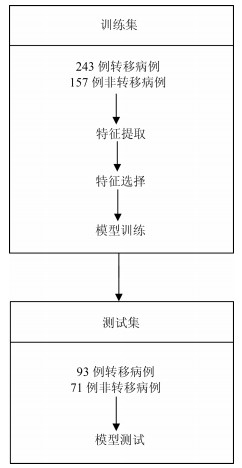
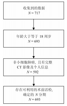
我们收集了广东省人民医院2007年5月至2014年6月期间的717例肺癌病例.这些病人在签署知情同意书后, 自愿提供自己的信息作为研究使用.为了充分利用收集到的数据对非小细胞肺癌淋巴结转移预测, 即对$N1-N3$与$N0$进行有效区分, 我们对收集的数据设置了三个入组标准: 1)年龄大于等于18周岁, 此时的肺部已经发育完全, 消除一定的干扰因素; 2)病理诊断为非小细胞肺癌无其他疾病干扰, 并有完整的CT (Computed tomography)增强图像及个人基本信息; 3)有可利用的术前病理组织活检分级用于确定N分期.经筛选, 共564例病例符合进行肺癌淋巴结转移预测研究的要求(如图 1).
为了得到有价值的结果, 考虑到数据的分配问题, 为了保证客观性, 防止挑数据的现象出现, 在数据分配上, 训练集与测试集将按照时间进行划分, 并以2013年1月为划分点.得到训练集: 400例, 其中, 243例正样本$N1-N3$, 157例负样本$N0$; 测试集: 164例, 其中, 93例正样本, 71例负样本.
1.2 病灶分割
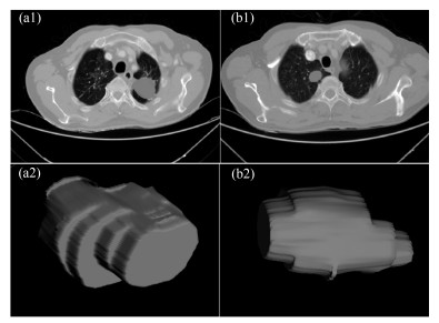
在进行特征提取工作前, 首先要对肿瘤病灶进行分割.医学图像分割的金标准是需要有经验的医生进行手动勾画的结果.但手动分割无法保证每次的分割结果完全一致, 且耗时耗力, 尤其是在数据量很大的情况下.因此, 手动分割不是最理想的做法.在本文中, 使用的自动图像分割算法为基于雪橇的自动区域生长分割算法[11], 该算法首先选定最大切片层的种子点, 这时一般情况下最大切片为中间层的切片, 然后估计肿瘤的大小即直径, 作为一个输入参数, 再自动进行区域生长得到每个切片的肿瘤如图 2(a1), (b1), 之后我们进行雪橇滑动到邻接的上下两个切面, 进行分割, 这样重复上述的区域生长即滑动切片, 最终分割得到多个切片的的肿瘤区域, 我们将肿瘤切面层进行组合, 得到三维肿瘤如图 2(a2), (b2).
1.3 特征的提取与筛选
利用影像组学处理方法, 从分割得到的肿瘤区域中总共提取出386个特征.这些特征可分为四组:三维形状特征, 表面纹理特征, Gabor特征和小波特征[12-13].形状特征通过肿瘤体积、表面积、体积面积比等特征描述肿瘤在空间和平面上的信息.纹理特征通过统计三维不同方向上像素的规律, 通过不同的分布规律来表示肿瘤的异质性. Gabor特征指根据特定方向, 特定尺度筛选出来的纹理信息.
小波特征是指原图像经过小波变换滤波器后的纹理特征.在模式识别范畴中, 高维特征会增加计算复杂度, 此外, 高维的特征往往存在冗余性, 容易造成模型过拟合.因此, 本位通过特征筛选方法首先对所有特征进行降维处理.
本文采用$L$1正则化Lasso进行特征筛选, 对于简单线性回归模型定义为:
$$ \begin{equation} f(x)=\sum\limits_{j=1}^p {w^jx^j} =w^\mathrm{T}x \end{equation} $$ (1) 其中, $x$表示样本, $w$表示要拟合的参数, $p$表示特征的维数.
要进行参数$w$学习, 应用二次损失来表示目标函数, 即:
$$ \begin{equation} J(w)=\frac{1}{n}\sum\limits_{i=1}^n{(y_i-f(x_i)})^2= \frac{1}{n}\vert\vert\ {{y}-Xw\vert\vert}^2 \end{equation} $$ (2) 其中, $X$是数据矩阵, $X=(x_1 , \cdots, x_n)^\mathrm{T}\in {\bf R}^{n\times p}$, ${y}$是由标签组成的列向量, ${y}=(y_1, \cdots, y_n )^\mathrm{T}$.
式(2)的解析解为:
$$ \begin{equation} \hat{w}=(X^\mathrm{T}X)^{-1}X^\mathrm{T}{y} \end{equation} $$ (3) 然而, 若$p\gg n$, 即特征维数远远大于数据个数, 矩阵$X^\mathrm{T}X$将不是满秩的, 此时无解.
通过Lasso正则化, 得到目标函数:
$$ \begin{equation} J_L(w)=\frac{1}{n} \vert\vert{y}-Xw\vert\vert^2+\lambda\vert\vert w\vert\vert _1 \end{equation} $$ (4) 目标函数最小化等价为:
$$ \begin{equation} \mathop {\min }\limits_w \frac{1}{n} \vert\vert{y}-Xw\vert\vert^2, \, \, \, \, \, \, \, \mathrm{s.t.}\, \, \vert \vert w\vert \vert _1 \le C \end{equation} $$ (5) 为了使部分特征排除, 本文采用$L$1正则方法进行压缩.二维情况下, 在$\mbox{(}w^1, w^2)$平面上可画出目标函数的等高线, 取值范围则为平面上半径为$C$的$L$1范数圆, 等高线与$L$1范数圆的交点为最优解. $L$1范数圆和每个坐标轴相交的地方都有"角''出现, 因此在角的位置将产生稀疏性.而在维数更高的情况下, 等高线与L1范数球的交点除角点之外还可能产生在很多边的轮廓线上, 同样也会产生稀疏性.对于式(5), 本位采用近似梯度下降(Proximal gradient descent)[14]算法进行参数$w$的迭代求解, 所构造的最小化函数为$Jl=\{g(w)+R(w)\}$.在每次迭代中, $Jl(w)$的近似计算方法如下:
$$ \begin{align} J_L (w^t+d)&\approx \tilde {J}_{w^t} (d)=g(w^t)+\nabla g(w^t)^\mathrm{T}d\, +\nonumber\\ &\frac{1} {2d^\mathrm{T}(\frac{I }{ \alpha })d}+R(w^t+d)=\nonumber\\ &g(w^t)+\nabla g(w^t)^\mathrm{T}d+\frac{{d^\mathrm{T}d} } {2\alpha } +\nonumber\\ &R(w^t+d) \end{align} $$ (6) 更新迭代$w^{(t+1)}\leftarrow w^t+\mathrm{argmin}_d \tilde {J}_{(w^t)} (d)$, 由于$R(w)$整体不可导, 因而利用子可导引理得:
$$ \begin{align} w^{(t+1)}&=w^t+\mathop {\mathrm{argmin}} \nabla g(w^t)d^\mathrm{T}d\, +\nonumber\\ &\frac{d^\mathrm{T}d}{2\alpha }+\lambda \vert \vert w^t+d\vert \vert _1=\nonumber\\ &\mathrm{argmin}\frac{1 }{ 2}\vert \vert u-(w^t-\alpha \nabla g(w^t))\vert \vert ^2+\nonumber\\ &\lambda \alpha \vert \vert u\vert \vert _1 \end{align} $$ (7) 其中, $S$是软阈值算子, 定义如下:
$$ \begin{equation} S(a, z)=\left\{\begin{array}{ll} a-z, &a>z \\ a+z, &a<-z \\ 0, &a\in [-z, z] \\ \end{array}\right. \end{equation} $$ (8) 整个迭代求解过程为:
输入.数据$X\in {\bf R}^{n\times p}, {y}\in {\bf R}^n$, 初始化$w^{(0)}$.
输出.参数$w^\ast ={\rm argmin}_w\textstyle{1 \over n}\vert \vert Xw-{y}\vert \vert ^2+\\ \lambda \vert\vert w\vert \vert _1 $.
1) 初始化循环次数$t = 0$;
2) 计算梯度$\nabla g=X^\mathrm{T}(Xw-{y})$;
3) 选择一个步长大小$\alpha ^t$;
4) 更新$w\leftarrow S(w-\alpha ^tg, \alpha ^t\lambda )$;
5) 判断是否收敛或者达到最大迭代次数, 未收敛$t\leftarrow t+1$, 并循环2)$\sim$5)步.
通过上述迭代计算, 最终得到最优参数, 而参数大小位于软区间中的, 将被置为零, 即被稀疏掉.
1.4 建立淋巴结转移影像组学标签与预测模型
本文使用LLR对组学特征进行降维并建模, 并使用10折交叉验证, 提高模型的泛化能力, 流程如图 3所示.
将本文使用的影像组学模型的预测概率(Radscore)作为独立的生物标志物, 并与临床指标中显著的特征结合构建多元Logistics模型, 绘制个性化预测的诺模图, 最后通过校正曲线来观察预测模型的偏移情况.
2. 结果
2.1 数据单因素分析结果
我们分别在训练集和验证集上计算各个临床指标与淋巴结转移的单因素P值, 计算方式为卡方检验, 结果见表 1, 发现吸烟与否和EGFR (Epidermal growth factor receptor)基因突变状态与淋巴结转移显著相关.
表 1 训练集和测试集病人的基本情况Table 1 Basic information of patients in the training set and test set基本项 训练集($N=400$) $P$值 测试集($N=164$) $P$值 性别 男 144 (36 %) 0.896 78 (47.6 %) 0.585 女 256 (64 %) 86 (52.4 %) 吸烟 是 126 (31.5 %) 0.030* 45 (27.4 %) 0.081 否 274 (68.5 %) 119 (72.6 %) EGFR 缺失 36 (9 %) 4 (2.4 %) 突变 138 (34.5 %) $ < $0.001* 67 (40.9 %) 0.112 正常 226 (56.5 %) 93 (56.7 %) 2.2 淋巴结转移影像组学标签
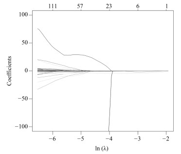
影像组学得分是每个病人最后通过模型预测后的输出值, 随着特征数的动态变化, 模型输出的AUC (Area under curve)值也随之变化, 如图 4所示, 使用R语言的Glmnet库可获得模型的参数$\lambda $的变化图.图中直观显示了参数$\lambda $的变化对模型性能的影响, 这次实验中模型选择了3个变量.如图 5所示, 横坐标表示$\lambda $的变化, 纵坐标表示变量的系数变化, 当$\lambda $逐渐变大时, 变量的系数逐渐减少为零, 表示变量选择的过程, 当$\lambda $越大表示模型的压缩程度越大.
 图 4 $\lambda $与变量数目对应走势Fig. 4 The trend of the parameters and the number of variables
通过套索回归方法, 自动的将变量压缩为3个, 其性能从图 4中也可发现, 模型的AUC值为最佳, 最终的特征如表 2所示. $V0$为截距项; $V179$为横向小波分解90度共生矩阵Contrast特征; $V230$为横向小波分解90度共生矩阵Entropy特征.
表 2 Lasso选择得到的参数Table 2 Parameters selected by LassoLasso选择的参数 含义 数值 $P$值 $V0$ 截距项 2.079115 $V179$ 横向小波分解90度共生矩阵Contrast特征(Contrast_2_90) 0.0000087 < 0.001*** $V230$ 横向小波分解90度共生矩阵Entropy特征(Entropy_3_180) $-$3.573315 < 0.001*** $V591$ 表面积与体积的比例(Surface to volume ratio) $-$1.411426 < 0.001*** $V591$为表面积与体积的比例; 将三个组学特征与$N$分期进行单因素分析, 其$P$值都是小于0.05, 表示与淋巴结转移有显著相关性.根据Lasso选择后的三个变量建立Logistics模型并计算出Rad-score, 详见式(9).并且同时建立SVM (Support vector machine)模型.
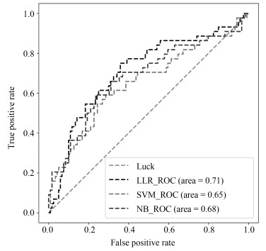
NB (Naive Bayesian)模型, 进行训练与预测, LLR模型训练集AUC为0.710, 测试集为0.712, 表现较优; 如表 3所示.将实验中使用的三个机器学习模型的结果进行对比, 可以发现, LLR的实验结果是最好的.
表 3 不同方法对比结果Table 3 Comparison results of different methods方法 训练集(AUC) 测试集(AUC) 召回率 LLR 0.710 0.712 0.75 SVM 0.698 0.654 0.75 NB 0.718 0.681 0.74 $$ \begin{equation} \begin{aligned} &\text{Rad-score}=2.328373+{\rm Contrast}\_2\_90\times\\ &\qquad 0.0000106 -{\rm entropy}\_3\_180\times 3.838207 +\\ &\qquad\text{Maximum 3D diameter}\times 0.0000002 -\\ &\qquad\text{Surface to volume ratio}\times 1.897416 \\ \end{aligned} \end{equation} $$ (9) 2.3 诺模图个性化预测模型
为了体现诺模图的临床意义, 融合Rad-score, 吸烟情况和EGFR基因因素等有意义的变量进行分析, 绘制出个性化预测的诺模图, 如图 7所示.为了给每个病人在最后得到一个得分, 需要将其对应变量的得分进行相加, 然后在概率线找到对应得分的概率, 从而实现非小细胞肺癌淋巴结转移的个性化预测.我们通过一致性指数(Concordance index, $C$-index)对模型进行了衡量, 其对应的$C$-index为0.724.
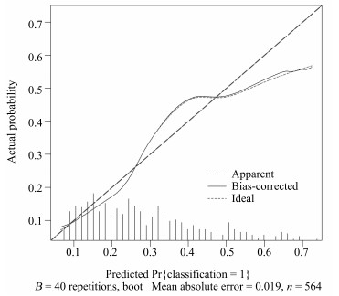
本文中使用校正曲线来验证诺模图的预测效果, 如图 8所示, 由校正曲线可以看出, 预测结果基本上没有偏离真实标签的结果, 表现良好, 因此, 该模型具有可靠的预测性能[15].
3. 结论
在构建非小细胞肺癌淋巴结转移的预测模型中, 使用LLR筛选组学特征并构建组学标签, 并与显著的临床特征构建多元Logistics模型, 绘制个性化预测的诺模图.其中LLR模型在训练集上的AUC值为0.710, 在测试集上的AUC值为0.712, 利用多元Logistics模型绘制个性化预测的诺模图, 得到模型表现能力$C$-index为0.724 (95 % CI: 0.678 $\sim$ 0.770), 并且在校正曲线上表现良好, 所以个性化预测的诺模图在临床决策上可起重要参考意义.[16].
-
图 4 $\lambda $与变量数目对应走势
Fig. 4 The trend of the parameters and the number of variables
表 1 训练集和测试集病人的基本情况
Table 1 Basic information of patients in the training set and test set
基本项 训练集($N=400$) $P$值 测试集($N=164$) $P$值 性别 男 144 (36 %) 0.896 78 (47.6 %) 0.585 女 256 (64 %) 86 (52.4 %) 吸烟 是 126 (31.5 %) 0.030* 45 (27.4 %) 0.081 否 274 (68.5 %) 119 (72.6 %) EGFR 缺失 36 (9 %) 4 (2.4 %) 突变 138 (34.5 %) $ < $0.001* 67 (40.9 %) 0.112 正常 226 (56.5 %) 93 (56.7 %)  下载: 导出CSV
表 2 Lasso选择得到的参数
Table 2 Parameters selected by Lasso
Lasso选择的参数 含义 数值 $P$值 $V0$ 截距项 2.079115 $V179$ 横向小波分解90度共生矩阵Contrast特征(Contrast_2_90) 0.0000087 < 0.001*** $V230$ 横向小波分解90度共生矩阵Entropy特征(Entropy_3_180) $-$3.573315 < 0.001*** $V591$ 表面积与体积的比例(Surface to volume ratio) $-$1.411426 < 0.001***
下载: 导出CSV
表 3 不同方法对比结果
Table 3 Comparison results of different methods
方法 训练集(AUC) 测试集(AUC) 召回率 LLR 0.710 0.712 0.75 SVM 0.698 0.654 0.75 NB 0.718 0.681 0.74
下载: 导出CSV
-
[1] Jemal A, Bray F, Center M M, Ferlay J, Ward E, Forman D. Global cancer statistics. CA Cancer Journal for Clinicians, 2011, 61(2):69-90 doi: 10.3322/caac.v61:2 [2] Howlader N, Noone A M, Krapcho M, Neyman N, Aminou R, Waldron W, et al. SEER cancer statistics review, 1975-2008. Bethesda, MD:National Cancer Institute[Online], available:http://seer.cancer.gov/csr/1975_2008/, August 1, 2015 [3] Glasgow S C, Bleier J I S, Burgart L J, Finne C O, Lowry A C. Meta-analysis of histopathological features of primary colorectal cancers that predict lymph node metastases. Journal of Gastrointestinal Surgery, 2012, 16(5):1019-1028 doi: 10.1007/s11605-012-1827-4 [4] Smith A J, Driman D K, Spithoff K, Hunter A, McLeod R S, Simunovic M, et al. Guideline for optimization of colorectal cancer surgery and pathology. Journal of Surgical Oncology, 2010, 101(1):5-12 doi: 10.1002/(ISSN)1096-9098 [5] Toiyama Y, Inoue Y, Shimura T, Fujikawa H, Saigusa S, Hiro J, et al. Serum angiopoietin-like protein 2 improves preoperative detection of lymph node metastasis in colorectal cancer. Anticancer Research, 2015, 35(5):2849-2856 http://www.wanfangdata.com.cn/details/detail.do?_type=perio&id=257db21275433b4ca2fe9da0f66d802c [6] Song J, Liu Z, Zhong W, Ma Z, Dong D, Liang C, et al. Nonsmall cell lung cancer:quantitative phenotypic analysis of CT images as a potential marker of prognosis. Scientific Reports, 2016, 6(1):Article No. 38282 doi: 10.1038/srep38282 [7] Gillies R J, Kinahan P E, Hricak H. Radiomics:images are more than pictures, they are data. Radiology, 2016, 278(2):563-577 doi: 10.1148/radiol.2015151169 [8] Kuo M D, Gollub J, Sirlin C B, Ooi C, Chen X. Radiogenomic analysis to identify imaging phenotypes associated with drug response gene expression programs in hepatocellular carcinoma. Journal of Vascular and Interventional Radiology, 2007, 18(7):821-830 doi: 10.1016/j.jvir.2007.04.031 [9] Lambin P, Rios-Velazquez E, Leijenaar R, Carvalho S, van Stiphout R G, Granton P, et al. Radiomics:extracting more information from medical images using advanced feature analysis. European Journal of Cancer, 2012, 48(4):441-446 doi: 10.1016/j.ejca.2011.11.036 [10] Sauerbrei W, Royston P, Binder H. Selection of important variables and determination of functional form for continuous predictors in multivariable model building. Statistics in Medicine, 2007, 26(30):5512-5528 doi: 10.1002/(ISSN)1097-0258 [11] Song J D, Yang C Y, Fan L, Wang K, Yang F, Liu S Y, et al. Lung lesion extraction using a toboggan based growing automatic segmentation approach. IEEE Transactions on Medical Imaging, 2015, 35(1):337-353 http://www.wanfangdata.com.cn/details/detail.do?_type=perio&id=25538c05c98e59d5f264491e0cd769c9 [12] Aerts H J W L, Velazquez E R, Leijenaar R T H, Parmar C, Grossmann P, Carvalho S, et al. Decoding tumour phenotype by noninvasive imaging using a quantitative radiomics approach. Nature Communications, 2014, 5:Article No. 4006 doi: 10.1038/ncomms5006 [13] Vickers A J, Cronin A M, Elkin E B, Gonen M. Extensions to decision curve analysis, a novel method for evaluating diagnostic tests, prediction models and molecular markers. BMC Medical Informatics and Decision Making, 2008, 8:Article No. 53 doi: 10.1186/1472-6947-8-53 [14] Zhang L J, Yang T B, Jin R, Zhou Z H. Stochastic proximal gradient descent for nuclear norm regularization. arXiv:1511.01664v2, January 1, 2015 [15] Huang Y Q, Liang C H, He L, Tian J, Liang C S, Chen X, et al. Development and validation of a radiomics nomogram for preoperative prediction of lymph node metastasis in colorectal cancer. Journal of Clinical Oncology, 2016, 34(18):2157-2164 doi: 10.1200/JCO.2015.65.9128 [16] Liang W H, Zhang L, Jiang G N, Wang Q, Liu L X, Liu D R, et al. Development and validation of a nomogram for predicting survival in patients with resected non-small-cell lung cancer. Journal of Clinical Oncology, 2015, 33(8):861-869 doi: 10.1200/JCO.2014.56.6661 -

 下载:
下载:

计量
- 文章访问数: 2013
- HTML全文浏览量: 413
- PDF下载量: 412
- 被引次数: 0
