基于数据特征融合的管网信息物理异常诊断方法

马大中; 胡旭光; 孙秋野; 郑君; 王睿

doi:10.16383/j.aas.2018.c180383

基于数据特征融合的管网信息物理异常诊断方法

doi: 10.16383/j.aas.2018.c180383

东北大学信息科学与工程学院沈阳 110819

基金项目:

国家自然科学基金重大项目 61627809

国家重点研发计划 2017YFF0108800

国家自然科学基金项目 61773109

中央高校基本科研业务费专项基金 N160404005

国家自然科学基金项目 61573094

详细信息

作者简介:
胡旭光  东北大学信息科学与工程学院博士研究生.主要研究方向为基于数据驱动的故障诊断, 信息物理系统的建模及优化控制.E-mail:1501004@stu.neu.edu.cn

孙秋野  东北大学信息科学与工程学院教授.主要研究方向为网络控制技术, 分布式控制技术, 分布式优化分析及其在能源互联网, 微网, 配电网等领域相关应用.E-mail:sunqiuye@mail.neu.edu.cn

郑君  东北大学信息科学与工程学院硕士研究生.主要研究方向为基于机器学习的综合能源系统故障检测与诊断.E-mail:ZJ623928036@163.com

王睿  东北大学信息科学与工程学院博士研究生.2016年于东北大学获得电气工程及其自动化专业学士学位.主要研究方向为能源互联网中分布式电源的协同优化及其电磁时间尺度稳定性分析.E-mail:1610232@stu.neu.edu.cn

通讯作者:
马大中东北大学信息科学与工程学院副教授.主要研究方向为故障诊断, 容错控制, 能源管理系统, 分布式发电系统、微网和能源互联网的优化与控制.本文通信作者.E-mail:madazhong@ise.neu.edu.cn

计量
- 文章访问数: 2138
- HTML全文浏览量: 532
- PDF下载量: 891
- 被引次数: 0
出版历程
- 收稿日期: 2018-05-31
- 录用日期: 2018-09-12
- 刊出日期: 2019-01-20

Cyber-physical Abnormity Diagnosis Method Using Data Feature Fusion for Pipeline Network

College of Information Science and Engineering, Northeastern University, Shenyang 110819

Funds:

Major Program of National Natural Foundation of China 61627809

National Key Research and Development Program of China 2017YFF0108800

National Natural Science Foundation of China 61773109

Fundamental Research Funds for the Central Universities N160404005

National Natural Science Foundation of China 61573094

More Information

Author Bio:
Ph. D. candidate at the College of Information Science and Engineering, Northeastern University. His research interest covers fault diagnosis based on data-driven, modeling and optimal control of cyber-physical system

Professor at the College of Information Science and Engineering, Northeastern University. His research interest covers network control technology, distributed control technology, distributed optimization analysis and various applications in energy internet, microgrid, power distribution network

Master student at the College of Information Science and Engineering, Northeastern University. His research interest covers fault detection and diagnosis of integrated energy system based on machine learning

Ph. D. candidate at the College of Information Science and Engineering, Northeastern University. He received his bachelor degree in electrical engineering and automation from Northeastern University in 2016. His research interest covers collaborative optimization of distributed generation and its stability analysis of electromagnetic timescale in energy internet

Corresponding author: MA Da-Zhong Associate professor at the College of Information Science and Engineering, Northeastern University. His research interest covers fault diagnosis, fault-tolerant control, energy management systems, and control and optimization of distributed generation systems, microgrids and energy internet. Corresponding author of this paper

摘要

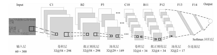
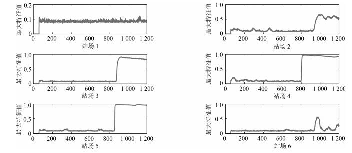
摘要: 随着管网物理空间和信息网络的深度融合，系统面临着物理和信息空间异常带来的运行风险.本文根据管网系统数据量大、耦合性强的特点，提出一种基于数据特征融合的信息物理异常诊断方法.首先通过站场信息数据构建信息增维矩阵并且通过矩阵预分析实现信息传输中断异常的判断.然后基于不同站场信息构建的信息增维协方差矩阵，通过矩阵特征值分布的变化情况对物理异常以及信息传输错误异常进行区分.在此基础上，为了对管网物理异常分类实现系统运行状态的有效分析，将管网信息增维协方差矩阵最大特征向量映射的二维图像作为输入，采用卷积神经网络进行研究，进而实现对物理异常的准确判断.最后通过某实际管网数据进行仿真分析，验证所提方法的有效性.
- 信息物理系统 /
- 输油管网 /
- 数据驱动 /
- 异常诊断
Abstract: With deep fusion between pipeline physical network and cyber network, the system is facing operational risks caused by cyber-physical anomalies. According to pipe network features of big data and strong coupling, this paper proposes a cyber-physical abnormity diagnosis method using data feature fusion for pipeline network. Firstly, a cyber augmented matrix can be built by station cyber data, and cyber interrupt is diagnosed by matrix pre-analysis. Furthermore, the cyber augmented covariance matrix is established in light of the different station cyber, and physical anomaly and cyber transmission error anomaly are distinguished from each other by the variation condition of the matrix eigenvalue distribution. To effectively analyze the operating state of the physical network anomaly classification, the two-dimensional images which are mapped by the maximum eigenvectors of the cyber augmented covariance matrix of the pipeline network are regarded as the input signals, meanwhile, a convolutional neural network is utilized to carry out the analysis, thus the accurate judgment of the physical anomaly is realized. Eventually, the effectiveness of the proposed method is demonstrated through the time-domain simulation result obtained on a practical pipeline network.
- Cyber-physical systems (CPS) /
- oil pipeline network /
- data driven /
- abnormity diagnosis
注释:

1) 本文责任编委曹向辉

HTML全文

图 1 管网信息物理系统结构

Fig. 1 CPS structure of pipeline network

下载: 全尺寸图片幻灯片

图 2 管网卷积神经网络模型

Fig. 2 structure of pipeline network

下载: 全尺寸图片幻灯片

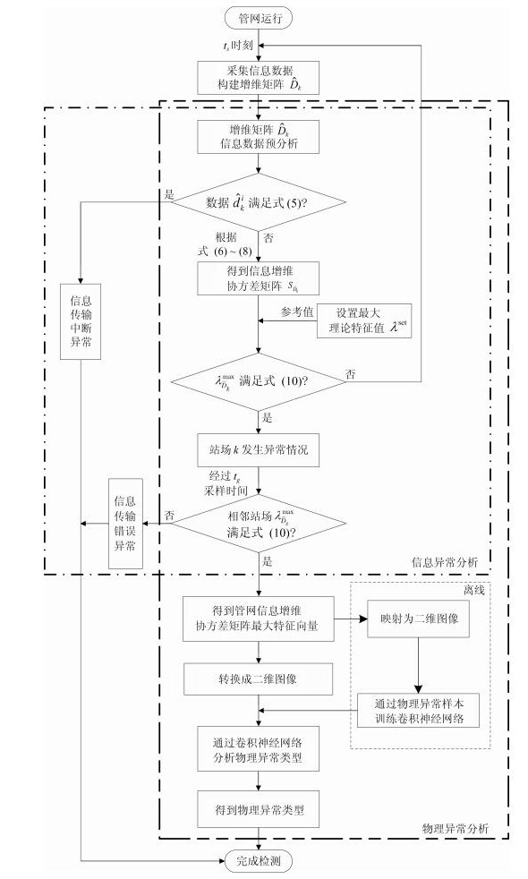
图 3 管网信息物理异常诊断流程图

Fig. 3 Flowchart of pipeline network for cyber-physical abnormity diagnosis

下载: 全尺寸图片幻灯片

图 4 管道信息中断压力曲线

Fig. 4 Pipeline cyber interrupt pressure

下载: 全尺寸图片幻灯片

图 5 管道信息错误压力曲线

Fig. 5 Pipeline cyber error pressure

下载: 全尺寸图片幻灯片

图 6 管道压力最大特征值曲线

Fig. 6 Max eigenvalue curves of pipeline pressure

下载: 全尺寸图片幻灯片

图 7 管网工况调整压力曲线

Fig. 7 Pipeline network operation adjustment pressure

下载: 全尺寸图片幻灯片

图 8 管网压力最大特征值曲线

Fig. 8 Max eigenvalue curves of pipeline network pressure

下载: 全尺寸图片幻灯片

图 9 卷积神经网络输出特征图

Fig. 9 Output feature of CNN

下载: 全尺寸图片幻灯片

图 10 管道泄漏压力曲线

Fig. 10 Pipeline leakage pressure

下载: 全尺寸图片幻灯片

图 11 管道压力最大特征值曲线

Fig. 11 Max eigenvalue curves of pipeline network pressure

下载: 全尺寸图片幻灯片

图 12 卷积神经网络输出特征图

Fig. 12 Output feature of CNN

下载: 全尺寸图片幻灯片

图 13 管道泄漏压力曲线

Fig. 13 Pipeline leakage pressure

下载: 全尺寸图片幻灯片

图 14 管道压力最大特征值曲线

Fig. 14 Max eigenvalue curve of pipeline network pressure

下载: 全尺寸图片幻灯片

图 15 卷积神经网络输出特征图

Fig. 15 Output feature of CNN

下载: 全尺寸图片幻灯片

表 1 物理异常统计结果

Table 1 The statistical result of physical abnormity

待识别类型	正确分类数	错误分类数	精度(%)
工况调整	2 696	104	96.3
泄漏	2 355	145	94.2

下载: 导出CSV

表 2 不同方法物理异常精度对比

Table 2 Comparison of accuracy among different methods

诊断方法	灵敏度	特异度	准确率
本文	94.2 %	96.3 %	95.3 %
文献[7]	91.0 %	88.6 %	89.7 %
BPNN	92.4 %	91.8 %	92.1 %
SVM	93.0 %	92.6 %	92.8 %

下载: 导出CSV

表 3 不同方法物理异常计算时间对比

Table 3 Comparison of computing time among different methods

诊断方法	训练时间	测试时间
本文	438.7582 s	$1.6701\times10^{-2}$ s
文献[7]	20.1538 s	$2.1252\times10^{-6}$ s
BPNN	16.9072 s	$8.6301\times10^{-7}$ s
SVM	1.4099 s	$1.9650\times10^{-5}$ s

下载: 导出CSV

参考文献(21)

[1]	王中杰, 谢璐璐.信息物理融合系统研究综述.自动化学报, 2011, 37(10):1157-1166 http://www.aas.net.cn/CN/abstract/abstract17604.shtml Wang Zhong-Jie, Xie Lu-Lu. Cyber-physical systems:a survey. Acta Automatica Sinica, 2011, 37(10):1157-1166 http://www.aas.net.cn/CN/abstract/abstract17604.shtml
[2]	温景容, 武穆清, 宿景芳.信息物理融合系统.自动化学报, 2012, 38(4):507-517 http://www.aas.net.cn/CN/abstract/abstract17704.shtml Wen Jing-Rong, Wu Mu-Qing, Su Jing-Fang. Cyber-physical system. Acta Automatica Sinica, 2012, 38(4):507-517 http://www.aas.net.cn/CN/abstract/abstract17704.shtml
[3]	Park K J, Zheng R, Liu X. Cyber-physical systems:milestones and research challenges. Computer Communications, 2012, 36(1):1-7 http://d.old.wanfangdata.com.cn/Periodical/jsjyy2013z2001
[4]	李健, 陈世利, 黄新敬, 曾周末, 靳世久.长输油气管道泄漏监测与准实时检测技术综述.仪器仪表学报, 2016, 37(8):1747-1760 doi: 10.3969/j.issn.0254-3087.2016.08.006 Li Jian, Chen Shi-Li, Huang Xin-Jing, Zeng Zhou-Mo, Jin Shi-Jiu. Review of leakage monitoring and quasi real-time detection technologies for long gas & oil pipelines. Chinese Journal of Scientific Instrument, 2016, 37(8):1747-1760 doi: 10.3969/j.issn.0254-3087.2016.08.006
[5]	刘金海, 冯健.基于模糊分类的流体管道泄漏故障智能检测方法研究.仪器仪表学报, 2011, 32(1):26-32 http://d.old.wanfangdata.com.cn/Periodical/yqyb201101005 Liu Jin-Hai, Feng Jian. Research on leak fault intelligent detection method for fluid pipeline based on fuzzy classification. Chinese Journal of Scientific Instrument, 2011, 32(1):26-32 http://d.old.wanfangdata.com.cn/Periodical/yqyb201101005
[6]	刘炜, 刘宏昭.基于结构相似度的管道泄漏检测定位法.中南大学学报(自然科学版), 2017, 48(1):134-140 http://d.old.wanfangdata.com.cn/Periodical/zngydxxb201701019 Liu Wei, Liu Hong-Zhao. Pipeline leak detection and location method based on structural similarity criteria. Journal of Central South University (Science and Technology), 2017, 48(1):134-140 http://d.old.wanfangdata.com.cn/Periodical/zngydxxb201701019
[7]	刘金海, 臧东, 汪刚.基于Markov特征的油气管道泄漏检测与定位方法.仪器仪表学报, 2017, 38(4):944-951 doi: 10.3969/j.issn.0254-3087.2017.04.020 Liu Jin-Hai, Zang Dong, Wang Gang. Leakage detection and location method of oil and gas pipelines based on Markov features. Chinese Journal of Scientific Instrument, 2017, 38(4):944-951 doi: 10.3969/j.issn.0254-3087.2017.04.020
[8]	阚哲, 郎宪明, 王晓蕾.基于信息物理系统架构分支管道泄漏定位.信息与控制, 2018, 47(1):22-28 http://d.old.wanfangdata.com.cn/Periodical/xxykz201801005 Kan Zhe, Lang Xian-Ming, Wang Xiao-Lei. Leakage location of branch pipeline based on cyber-physical system architecture. Information and Control, 2018, 47(1):22-28 http://d.old.wanfangdata.com.cn/Periodical/xxykz201801005
[9]	王伟凝, 王励, 赵明权, 蔡成加, 师婷婷, 徐向民.基于并行深度卷积神经网络的图像美感分类.自动化学报, 2016, 42(6):904-914 http://www.aas.net.cn/CN/abstract/abstract18881.shtml Wang Wei-Ning, Wang Li, Zhao Ming-Quan, Cai Cheng-Jia, Shi Ting-Ting, Xu Xiang-Min. Image aesthetic classification using parallel deep convolutional neural networks. Acta Automatica Sinica, 2016, 42(6):904-914 http://www.aas.net.cn/CN/abstract/abstract18881.shtml
[10]	常亮, 邓小明, 周明全, 武仲科, 袁野, 杨硕, 等.图像理解中的卷积神经网络.自动化学报, 2016, 42(9):1300-1312 http://www.aas.net.cn/CN/abstract/abstract18919.shtml Chang Liang, Deng Xiao-Ming, Zhou Ming-Quan, Wu Zhong-Ke, Yuan Ye, Yang Shuo, et al. Convolutional neural networks in image understanding. Acta Automatica Sinica, 2016, 42(9):1300-1312 http://www.aas.net.cn/CN/abstract/abstract18919.shtml
[11]	李勇, 林小竹, 蒋梦莹.基于跨连接LeNet-5网络的面部表情识别.自动化学报, 2018, 44(1):176-182 http://www.aas.net.cn/CN/abstract/abstract19213.shtml Li Yong, Lin Xiao-Zhu, Jiang Meng-Ying. Facial expression recognition with cross-connect LeNet-5 network. Acta Automatica Sinica, 2018, 44(1):176-182 http://www.aas.net.cn/CN/abstract/abstract19213.shtml
[12]	Kang J, Park Y J, Lee J, Wang S H, Eom D S. Novel leakage detection by ensemble CNN-SVM and graph-based localization in water distribution systems. IEEE Transactions on Industrial Electronics, 2018, 65(5):4279-4289 doi: 10.1109/TIE.2017.2764861
[13]	Feng J, Li F M, Lu S X, Liu J H, Ma D Z. Injurious or noninjurious defect identification from MFL images in pipeline inspection using convolutional neural network. IEEE Transactions on Instrumentation and Measurement, 2017, 66(7):1883-1892 doi: 10.1109/TIM.2017.2673024
[14]	Lu S X, Feng J, Zhang H G, Liu J H, Wu Z N. An estimation method of defect size from MFL image using visual transformation convolutional neural network. IEEE Transactions on Industrial Informatics, DOI: 10.1109/TⅡ.2018.2828811
[15]	杨理践, 曹辉.基于深度学习的管道焊缝法兰组件识别方法.仪器仪表学报, 2018, 39(2):193-202 http://epub.cnki.net/grid2008/detail.aspx?filename=YQXB201802023&dbname=DKFX2018 Yang Li-Jian, Cao Hui. Deep learning based weld and flange identification in pipeline. Chinese Journal of Scientific Instrument, 2018, 39(2):193-202 http://epub.cnki.net/grid2008/detail.aspx?filename=YQXB201802023&dbname=DKFX2018
[16]	韩春宇, 黄春, 陈飞, 南兵.东临复线水击保护实例分析.油气储运, 2008, 27(2):53-55 http://d.old.wanfangdata.com.cn/Periodical/yqcy200802015 Han Chun-Yu, Huang Chun, Chen Fei, Nan Bing. Surge protection case for Dongying-Linyi parallel oil pipeline. Oil & Gas Storage and Transportation, 2008, 27(2):53-55 http://d.old.wanfangdata.com.cn/Periodical/yqcy200802015
[17]	邓忠华, 尤冬青, 郭晔, 李洪军, 李岳, 闻峰, 等.石兰原油管道通信系统中断运行保护.油气储运, 2017, 36(5):543-547 http://d.old.wanfangdata.com.cn/Periodical/yqcy201705011 Deng Zhong-Hua, You Dong-Qing, Guo Ye, Li Hong-Jun, Li Yue, Wen Feng, et al. Interruption protection of communication system in Shikong-Lanzhou Crude Oil Pipeline. Oil & Gas Storage and Transportation, 2017, 36(5):543-547 http://d.old.wanfangdata.com.cn/Periodical/yqcy201705011
[18]	何兆洋, 尚义, 何丽萍, 黎春, 殷素娜.漠大原油管道SCADA通讯中断原因及应对措施.油气储运, 2014, 33(5):501-504 http://d.old.wanfangdata.com.cn/Periodical/yqcy201405010 He Zhao-Yang, Shang Yi, He Li-Ping, Li Chun, Yin Su-Na. Reasons and solutions of SCADA communication interruption in Mohe-Daqing Crude Oil Pipeline. Oil & Gas Storage and Transportation, 2014, 33(5):501-504 http://d.old.wanfangdata.com.cn/Periodical/yqcy201405010
[19]	Bai Z D, Silverstein J W. Spectral Analysis of Large Dimensional Random Matrices (Second Edition). New York: Springer-Verlag, 2010.
[20]	Lecun Y, Bottou L, Bengio Y, Haffner P. Gradient-based learning applied to document recognition. Proceedings of the IEEE, 1998, 86(11):2278-2324 doi: 10.1109/5.726791
[21]	周飞燕, 金林鹏, 董军.卷积神经网络研究综述.计算机学报, 2017, 40(6):1229-1251 http://d.old.wanfangdata.com.cn/Periodical/jsjxb201706001 Zhou Fei-Yan, Jin Lin-Peng, Dong Jun. Review of convolutional neural network. Chinese Journal of Computers, 2017, 40(6):1229-1251 http://d.old.wanfangdata.com.cn/Periodical/jsjxb201706001

施引文献

资源附件(0)

访问统计

图(15) / 表(3)

计量

文章访问数: 2138
HTML全文浏览量: 532
PDF下载量: 891
被引次数: 0

姓名
邮箱
手机号码
标题
留言内容
验证码

留言板

基于数据特征融合的管网信息物理异常诊断方法

doi: 10.16383/j.aas.2018.c180383

通讯作者:
马大中东北大学信息科学与工程学院副教授.主要研究方向为故障诊断, 容错控制, 能源管理系统, 分布式发电系统、微网和能源互联网的优化与控制.本文通信作者.E-mail:madazhong@ise.neu.edu.cn

计量

Cyber-physical Abnormity Diagnosis Method Using Data Feature Fusion for Pipeline Network

计量

目录

留言板

基于数据特征融合的管网信息物理异常诊断方法

doi: 10.16383/j.aas.2018.c180383

通讯作者: 马大中 东北大学信息科学与工程学院副教授.主要研究方向为故障诊断, 容错控制, 能源管理系统, 分布式发电系统、微网和能源互联网的优化与控制.本文通信作者.E-mail:madazhong@ise.neu.edu.cn

计量

出版历程

Cyber-physical Abnormity Diagnosis Method Using Data Feature Fusion for Pipeline Network

计量

出版历程

目录

通讯作者:
马大中东北大学信息科学与工程学院副教授.主要研究方向为故障诊断, 容错控制, 能源管理系统, 分布式发电系统、微网和能源互联网的优化与控制.本文通信作者.E-mail:madazhong@ise.neu.edu.cn