

A Contour Detection Method Based on Visual Perception Mechanism in Primary Visual Pathway
-
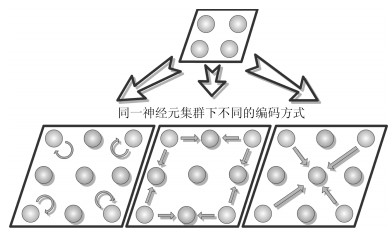
摘要: 考虑到初级视通路中视觉信息传递和处理过程中的特点, 本文提出了一种基于视觉感知机制的轮廓检测新方法.构建视觉信息局部细节检测与整体轮廓感知的不同路径.利用高斯导函数提取初级轮廓响应; 构建神经网络, 利用时空编码提高主体轮廓对比度; 然后, 利用非经典感受野的侧抑制作用抑制纹理背景; 另外, 针对轮廓信息强化以及检测鲁棒性的要求, 在视辐射区提出了一种信息冗余度增强编码机制; 最后, 将初级轮廓直接前馈至初级视皮层, 以达到轮廓响应的快速调节和完整性融合.以RuG40图库为实验对象, 经过非极大值抑制和阈值处理, 得到的轮廓二值图与基准轮廓图比较, 在整个数据集中的最优平均$P$指标和每张图的最优平均$P$指标分别为0.48和0.55, 并且FPS达到了1/2.结果表明本文方法能有效突出主体轮廓并抑制纹理背景, 为后续图像理解和分析提供了一种新的思路.Abstract: A new method of contour detection is proposed in this paper according to the characteristics of visual information transmission and processing which is based on visual perception mechanism in human primary visual pathway. Firstly, the spatio-temporal coding of neural information is realized on the basis of the Gaussian derivative function, and then the texture and background are suppressed by the non-classical receptive field. In addition, we propose a neural coding that can strengthen the redundancy of visual information in the optic radiation area to enhance the contour information and robustness of detecting. Finally, primary contour is fed forward to the primary visual cortex to achieve rapid adjustment of the contour response. In this paper, the RuG40 library is taken for processing, acquiring the contour detecting result through the non-maximal suppression and hysteresis threshold, and mean values $P$ of optimal parameters for whole dataset and each image are 0.48 and 0.55, respectively, compared with the ground truth. In addition, the FPS of algorithm reaches 1/2. The results indicate the new method in this paper can effectively highlight the principal contour and suppress texture region which will provide a new idea for subsequent image comprehension and analysis.
-
Key words:
- Contour detection /
- spatio-temporal coding /
- enhancement coding of information redundancy /
- feed forward
-
1. Introduction
For permanent magnet synchronous motor (PMSM) drive system, the measurement of instantaneous stator currents is required for successful operation of the feedback control. Generally two phase current sensors are installed in three phase voltage source inverters (VSI). Nevertheless, sudden severe failure of phase current sensors would result in over-current malfunction of the drive system. And if there is no protection scheme in the gate-drive circuit, the failure would lead to irrecoverable fault of power semiconductors in VSI, which would cause degradation of motor drive performance. Additionally, some minor failures (such as gain drift and nonzero offset) of phase current sensors would lead to torque pulsation synchronizing with the inverter output frequency [1]. The larger offset and scaling error of phase current sensors would bring about the worse performance of torque regulation. Moreover, if the offset and gain drift are above certain level, it would cause over-current trip under high speed and heavy load conditions [2]. So it is necessary to consider fault tolerant operation of phase current sensor failure.
The current sensorless technology, regarded as fault tolerant one, has been developed in the past few decades. Its core lies in that the physical fault current sensor is replaced with virtual sensor (or current estimator). This technology has several advantages such as high reliability and low cost as well as space and weight savings owing to omitting physical current sensor. Moreover, it allows the drive system to work in hostile environment.
As far as the current sensorless technique is concerned, three estimation solutions have been reported in the literature. The first one is a DC-link current-based approach which restructures phase currents with the information of the DC-link current and switching states in VSI [3]. Although it is a mainstream method, its unavoidable drawbacks are exposed: the duration of an active switching state may be so short that the DC-link current cannot be measured on one hand, on the other hand, there are immeasurable regions in the output voltage hexagon where the DC-link current sampling and reconstruction are limited or impossible to do [4]. In addition, the DC-link sensed current remains sensitive to the narrow pulse and further deteriorates if the cable capacitance causes spurious oscillations in the DC-link waveform. In order to provide high-accuracy phase current reconstruction over a wide range of operating conditions with a low current waveform, over the past years, many kinds of methods of improved PWM modulation strategy have been proposed for the single DC-link current sensor technique [5]$-$[14]. Although many improved methods show reasonable phase current reconstruction performance, these methods suffer from complicated algorithms [15]. The second one is an analytical model-based approach. In [16], on the basis of the voltage and flux equations of induction motor (IM) drive, the phase current is estimated by using the synchronous reference frame variables under single phase current sensor condition. In [17], by the discrete voltage equations of PMSM drive, the phase currents are estimated. Although it is easier to implement than the first one, the method is not robust against the variation of system parameters. The third one is an adaptive observer-based approach. In [18], the phase current is reconfigured for IM drive using single phase current sensor, while in [19], the phase currents are reconfigured for PMSM drive without any phase current sensors. Compared with the first two solutions, the third solution has stronger robustness against the variation of system parameters [20], [21]. For PMSM drive system when only one phase current sensor is available, the remaining two phase currents estimation based on an adaptive observer must be studied, which is required to perform current feedback control. However, there is no literature on such strategy.
For PMSM drive system, model predictive torque control (MPTC) is an emerging control strategy [22]$-$[29]. Its main objective is to control instantaneous torque and stator flux with high accuracy and thus MPTC plays an important role to ensure the quality of the torque and speed control. MPTC adopts the principle of model predictive control (MPC) and can provide high dynamic performance and low stator current harmonics.
For conventional proportional-integral(PI)-based MPTC PMSM drive system, its speed regulator employs the algorithm of PI. In general, PI may perform well under certain operating condition, but it does not work properly and thus degrades dynamic performance under other operating conditions such as variation of system parameters and external disturbances. To improve the robustness of the speed regulator, some techniques have been proposed in recent years [30]$-$[34]. Except these techniques, a global fast terminal sliding mode (GFTSM) control is an effective and practical one [35], [36], which is based on sliding mode theory and employs the fast terminal sliding mode in both the reaching stage and sliding stage. By adding the nonlinear function to the sliding mode surface, the GFTSM controller can enable drive system not only to be superiorly robust against system uncertainties and external disturbances but also to have quick response as well as high control precision. Even so, studies on GFTSM speed regulator are very few. In this paper, we propose replacement of PI with GFTSM for MPTC PMSM drive system.
In this paper, by referring to the adaptive approach and integrating the GFTSM method, a new GFTSM-based MPTC strategy with the adaptive observer is put forward for the PMSM drive system with single phase current sensor. The proposed adaptive observer presents a satisfactory tracking performance of the remaining two phase currents in the presence of stator resistance change caused by the temperature variation. And the designed GFTSM controller enhances the speed regulator's robustness against parameter uncertainty and external disturbance. On the basis of the above foundation, the synthesized MPTC PMSM drive control system achieves a high performance.
This paper is organized as follows: Dynamic model of PMSM drive is presented in Section 2. Section 3 gives the adaptive observer and GFTSM speed regulator design as well as MPTC design. Experimental results and analysis are presented in Section 4. Section 5 contains the conclusions.
Notation 1: The following nomenclature is used throughout this paper:
$ \begin{align*} \begin{array}{lll} R_{\rm s}:& &\mbox {Nominal phase resistance} \ \\ \psi_{\rm m}:&&\mbox{The permanent magnet flux} \ \\ \psi_{\rm s}:&&\mbox{Stator flux linkage}\\ p:&&\mbox{Number of pole pairs}\\ V_{\rm dc}:&&\mbox{DC bus voltage}\\ \omega_{\rm r}:&&\mbox{Rotor actual mechanical speed}\\ T_{\rm l}:&&\mbox{Load torque}\\ T_{\rm e}:&&\mbox{Electromagnetic torque}\\ J:&&\mbox{Moment of inertia}\\ B_{\rm m}:&&\mbox{Viscous friction coefficient}\\ T_{\rm f}:&&\mbox{Coulomb friction torque}\\ \theta:&&\mbox{Rotor electrical angular position}\\ i:&&\mbox{Stator current}\\ u:&&\mbox{Stator voltage}\\ L:&&\mbox{Stator inductance}.\\ \end{array} \end{align*} $
Notation 2: The following symbol is used throughout this paper. $\bullet_{\rm d}$, $\bullet_{\rm q}$, $\bullet_{\alpha}$ and $\bullet_{\beta}$ are used to denote the $d$-axis, $q$-axis, $\alpha$-axis, and $\beta$-axis component of $\bullet$, respectively; $\bullet^{\ast}$ is used to denote the reference values of $\bullet$; $\hat{\bullet}$ is used to denote the estimate of $\bullet$; $\tilde{\bullet}$ is used to denote the parameter estimation error of $\bullet$; $\bullet^{k}$ and $\bullet^{k+1}$ are used to denote the instantaneous value at $k$th and ($k+1$)th of $\bullet$, respectively.
2. Dynamic Models of Three-phase PMSM Drive
As for three-phase PMSM drive, the models in rotor synchronous reference frame ($dq$-frame) and two-phase stationary reference frame ($\alpha\beta$-frame) are expressed as follows, respectively:
$ \begin{align} \label{eq:1} % eq:(1) \begin{cases} \dfrac{{d}i_{\rm d}}{{d}t}&=\dfrac{1}{L_{\rm d}} \left(u_{\rm d}-R_{\rm s}i_{\rm d}+p\omega_{\rm r}L_{\rm q}i_{\rm q}\right) \\[3mm] \dfrac{{d}i_{\rm q}}{{d}t}&=\dfrac{1}{L_{\rm q}}\left(u_{\rm q}-R_{\rm s}i_{\rm q}+p\omega_{\rm r} (L_{\rm d}i_{\rm d}+\psi_{\rm m})\right) \end{cases}\end{align} $
(1) $\begin{align} \begin{cases} \dfrac{{d}i_{\alpha}}{{d}t}&=\dfrac{1}{L_{\alpha}} \left(u_{\alpha}-R_{\rm s}i_{\alpha}+p\omega_{\rm r}\psi_{\rm m} \sin\theta\right) \\[3mm] \dfrac{{d}i_{\beta}}{{d}t}&=\dfrac{1}{L_{\beta}} \left(u_{\beta}-R_{\rm s}i_{\beta}-p\omega_{\rm r}\psi_{\rm m}\cos\theta\right) \end{cases} \end{align} $
(2) and the mechanical equation is expressed as
$ \begin{align} \dfrac{{d}\omega_{\rm r}}{{d}t}=\dfrac{1}{J}(T_{\rm e}-T_{\rm l}-B_{\rm m}\omega_{\rm r}-T_{\rm f}) \end{align} $
(3) where the electromagnetic torque $T_{\rm e}$ is expressed as
$\begin{align} T_{\rm e}=\frac{3{ p}}{2} \left[\psi_{\rm m}i_{\rm q}+(L_{\rm d}-L_{\rm q})i_{\rm d}i_{\rm q}\right]. \end{align} $
(4) 3. Design of GFTSM-based MPTC PMSM Drive System With Adaptive Observer
The objective of GFTSM-based MPTC using adaptive observer is that the PMSM drive system can work reliably and its speed and torque can be controlled not only to have satisfactory performance but also to be strongly robust against parameters variation and external disturbance. The schematic of the proposed control system is shown in Fig. 1. Our design task concentrates on adaptive observer, GFTSM speed regulator and MPTC as follows.
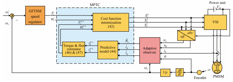 图 1 Block diagram of GFTSM-based MPTC PMSM drive system with adaptive observer.Fig. 1 Block diagram of GFTSM-based MPTC PMSM drive system with adaptive observer.
3.1 Adaptive Observer Design
The proposed adaptive observer is to estimate the remaining two phase currents and stator resistance when single phase current sensor is available. In the design process, assume the following conditions.
1) Only phase-$b$ current can be measured and the remaining two phase current sensors are not available.
2) Due to heating during operating of the motor, the stator resistance $R_{\rm s}$ is considered as a time-varying parameter.
3) There is no saturation in the magnetic circuit.
For surface-mounted PMSM drive, $L_{\rm d}=L_{\rm q}=L_{\alpha}= L_{\beta}$ $=$ $L$. The $\alpha$-axis in $\alpha\beta$-frame is oriented along phase-$a$ axis in three-phase stationary reference frame ($abc$-frame). The $abc$-axis stator currents in $abc$-frame can be obtained from the $\alpha\beta$-axis ones in $\alpha\beta$-frame by the following transformation matrix:
$ \left[ \begin{matrix} {{i}_{\rm{a}}} \\ {{i}_{\rm{b}}} \\ {{i}_{\rm{c}}} \\ \end{matrix} \right]=\left[ \begin{matrix} 1 & 0 \\ -\frac{1}{2} & \frac{\sqrt{3}}{2} \\ -\frac{1}{2} & -\frac{\sqrt{3}}{2} \\ \end{matrix} \right]\left[ \begin{matrix} {{i}_{\alpha }} \\ {{i}_{\beta }} \\ \end{matrix} \right] $
(5) where $i_{\rm a}$, $i_{\rm b}$, and $i_{\rm c}$ are $abc$-axis stator currents in $abc$-frame. From (5), the following equation can be given,
$ \begin{align} % eq:(6) i_{\rm b}=-\frac{1}{2} i_\alpha+\frac{\sqrt{3}}{2}i_\beta. \end{align} $
(6) Taking (2) into account, the time derivative of (6) is deduced as follows:
$ \begin{align} % eq:(7) \frac{{d}i_{\rm b}}{{d}t}& =\dfrac{\sqrt{3}}{2L}\left[u_\beta-R_{\rm s}\left(\frac{1}{ \sqrt{3}}i_\alpha+\frac{2}{ \sqrt{3}}i_{\rm b}\right)-p\omega_{\rm r}\psi_m\cos\theta\right]\notag\\ & \quad -\frac{1}{2L} (u_{\alpha}-R_{\rm s}i_{\alpha}+p\omega_{\rm r}\psi_{\rm m}\sin\theta)\notag\\ &=\frac{\sqrt{3}u_\beta-u_{\alpha}-2R_{\rm s}i_{\rm b}-p\omega_{\rm r}\psi_{\rm m}(\sqrt{3}\cos\theta+\sin\theta)} {2L}. \end{align} $
(7) The following adaptive observer is proposed in order to estimate phase-$b$ current,
$ \begin{align} % eq:(8) \frac{{d}\hat{i}_{\rm b}}{{d}t}& =\frac{\sqrt{3}}{ 2L}\left[u_\beta-\hat{R}_{\rm s}\left(\frac{1}{ \sqrt{3}}\hat{i}_\alpha+\frac{2}{ \sqrt{3}}i_{\rm b}\right)-p\omega_{\rm r}\psi_m\cos\theta\right]\notag\\ & \quad -\frac{1}{ 2L}\left(u_{\alpha}-\hat{R}_{\rm s}\hat{i}_{\alpha}+p\omega_{\rm r}\psi_{\rm m}\sin\theta\right)-k_1f(\tilde{i}_{\rm b})-k_2\tilde{i}_{\rm b}\notag\\ & =\frac{1}{2L}\left[\sqrt{3}u_\beta-u_{\alpha}-2\hat{R}_{\rm s}i_{\rm b}-p\omega_{\rm r}\psi_{\rm m}(\sqrt{3}\cos\theta + \sin\theta)\right]\notag\\ &\quad-k_1f(\tilde{i}_{\rm b})-k_2\tilde{i}_{\rm b} \end{align} $
(8) where $k_1f(\tilde{i}_{\rm b})$ and $k_2\tilde{i}_{\rm b}$ are correctors, and $k_1$ and $k_2$ are the positive observer gains, and $f(\cdot)$ denotes the nonlinear function of phase-$b$ current estimation error $\tilde{i}_{\rm b}$, which is defined as
$ \begin{align} % eq:(9) \tilde{i}_{\rm b}=\hat{i}_{\rm b}-i_{\rm b}. \end{align} $
(9) Define the following stator resistance estimation error,
$ \begin{align} % eq:(10) \tilde{R}_{\rm s}=\hat{R}_{\rm s}-R_{\rm s}. \end{align} $
(10) By subtracting (8) from (7), the dynamics equation of the phase-$b$ current estimation error is given as follows:
$ \begin{align} % eq:(11) \frac{{d}\tilde{i}_{\rm b}}{{d}t}=-\frac{1}{ L}\tilde{R}_{\rm s}i_{\rm b}-k_1f(\tilde{i}_{\rm b})-k_2\tilde{i}_{\rm b}. \end{align} $
(11) In order to determine the adaptive law of the stator resistance and the observer gains, construct the candidate Lyapunov function as
$ \begin{align} % eq:(12) V_1=\frac{1}{ 2}\left(\tilde{i}_{\rm b}^2+{1\over r}\tilde{R}_{\rm s}^2\right) \end{align} $
(12) where $r$ is constant positive scalar.
The time derivative of (12) is obtained as follows:
$ \begin{align} % eq:(13) \frac{{d}{V_1}}{{d}t}=-k_2\tilde{i}_{\rm b}^2-k_1f(\tilde{i}_{\rm b})\tilde{i}_{\rm b}+\tilde{R}_{\rm s}\left(\frac{1}{ r}\frac{{d}\tilde{R}_{\rm s}}{{d}t}-\frac{1}{ L}i_{\rm b}\tilde{i}_{\rm b}\right). \end{align} $
(13) If we define following equality,
$ \begin{align} % eq:(14) \frac{1}{r}\frac{{d}\tilde{R}_{\rm s}}{{d}t}-\frac{1}{ L}i_{\rm b}\tilde{i}_{\rm b}=0. \end{align} $
(14) Equation (13) can be rewritten as below:
$ \begin{align} % eq:(15) \frac{{d}{V_1}}{{d}t}=-k_2\tilde{i}_{\rm b}^2-k_1f(\tilde{i}_{\rm b})\tilde{i}_{\rm b}. \end{align} $
(15) To render $\dot V_{1}$ negative, we assume
$ \begin{align} % eq:(16) f(\tilde{i}_{\rm b})={\rm sign}(\tilde{i}_{\rm b}). \end{align} $
(16) As a result, the following inequality is satisfied
$ \frac{{d}{V_1}}{{d}t}<0. $
By Lyapunov stability theorem, dynamic system (11) is stable, which means that both $\tilde{i}_{\rm b}$ and $\tilde{R}_{\rm s}$ can converge to zero. Since the variation of the stator resistance in the observer time scale is negligible, i.e.,
$ \frac{{d}R_{\rm s}}{{d}t}\approx 0 $
then the following formula holds
$ \begin{align} % eq:(17) \frac{{d}\tilde{R}_{\rm s}}{{d}t}=\frac{{d}\hat{R}_{\rm s}}{{d}t}-\frac{{d}R_{\rm s}}{{d}t}\approx\frac{{d}\hat{R}_{\rm s}}{{d}t}. \end{align} $
(17) Therefore, from (14), the adaptive mechanism of the stator resistance is derived as follows:
$ \begin{align} % eq:(18) \hat{R}_{\rm s}={r\over L}\int(i_{\rm b}\tilde{i}_{\rm b}){ d}t. \end{align} $
(18) With the adaptive mechanism in (18), the estimation value of the stator resistance can converge to its real value.
In order to improve the estimation accuracy of the stator resistance and to ensure a null steady error, on the basis of PI strategy, (18) is modified as below:
$ \begin{align} % eq:(19) \hat{R}_{\rm s}=\frac{r}{ L}\left\{{K_{P(R_{\rm s})}[i_{\rm b}(\hat{i}_{\rm b}-i_{\rm b})]+K_{I(R_{\rm s})}\int[i_{\rm b}(\hat{i}_{\rm b}-i_{\rm b})]{d}t}\right\} \end{align} $
(19) where $K_{P(R_{\rm s})}$ and $K_{I(R_{\rm s})}$ are proportional and integral scalars, respectively.
By replacing $R_{\rm s}$ in (2) with $\hat{R}_{\rm s}$ in (19), the $\alpha\beta$-axis currents observers can be constructed as follows:
$ \begin{align} % eq:(20) \begin{cases} \dfrac{{d}\hat{i}_{\alpha}}{{d}t}=\dfrac{1}{ L} \left(u_{\alpha}-\hat{R}_{\rm s}\hat{i}_{\alpha}+p\omega_{\rm r} \psi_{\rm m}\sin\theta\right) \\[3mm] \dfrac{{d}\hat{i}_{\beta}}{{d}t} =\dfrac{1}{ L}\left(u_{\beta}-\hat{R}_{\rm s}\hat{i}_{\beta} -p\omega_{\rm r}\psi_{\rm m}\cos\theta\right). \end{cases} \end{align} $
(20) By combining (8), (19) and (20), the block diagram of the designed adaptive observer is established as shown in Fig. 2, which treats the stator voltages, rotor electrical position and speed as the inputs, the $dq$-axis currents and stator resistance as outputs when only phase-$b$ current is measured.
 图 2 Block diagram of the proposed adaptive observer.Fig. 2 Block diagram of the proposed adaptive observer.
Remark 1: From Fig. 2, it can be seen that estimating the phase-$b$ current is a key step and primary premise in construction of the adaptive observer. The error between the phase-$b$ measured current and its estimated value must be guaranteed to converge towards zero.
Remark 2: From (8) and (19), it can be seen that although the coupling relationship between $\hat{i}_{\rm b}$ and $\hat{R}_{\rm s}$ exists, we do not need to decouple them in the design process. In fact, the phase-$b$ current estimation (8) and the stator resistance adaptive law (19) are implemented and solved all together.
Remark 3: The convergence rate of the observer is dependent on the observer gains $k_1$ and $k_2$, which should be chosen to be large enough such that the observer responds as soon as possible.
Remark 4: The estimated $dq$-axis currents in Fig. 2 will be applied to MPTC as shown in Fig. 1.
Remark 5: From (5), the estimation of phase-$a$ current in $abc$-frame is equal to that of $\alpha$-axis current in $\alpha\beta$-frame as follows:
$ \begin{align} % eq:(21) \hat{i}_{\rm a}=\hat{i}_{\alpha}. \end{align} $
(21) Accordingly, the estimation of phase-$c$ current in $abc$-frame can be obtained as follows:
$ \hat{i}_{\rm c}=-(i_{\rm b}+\hat{i}_{\alpha}). $
Remark 6: The proposed adaptive observer is robust against only the stator resistance change. If other parameter uncertainties (such as stator inductance change and permanent magnet flux change, etc.) and unmodeled dynamics are required to be considered, then adaptive robust method with extended state observer can be borrowed from [20] and [33], which is our next research topic.
3.2 GFTSM Speed Regulator Design
3.2.1 GFTSM Design
Define the speed error as
$ e=\omega_{\rm r}^{\ast}-\omega_{\rm r}. $
Let
$ \begin{align} % eq:(22) x_1=e, ~~x_2=\dot{x}_{1}, ~~ u=\dot{T}_{\rm e}. \end{align} $
(22) Assume that $\omega_{\rm r}^{\ast}$ (or $\dot{\omega}_{\rm r}^{\ast}$), $T_{\rm l}$, $T_{\rm f}$ are constants and $\omega_{\rm r}$ has continuous second-order derivative. Then, the state equation of (3) can be expressed as following:
$ \begin{align} % eq:(23) \begin{cases} \dot{x}_{1}=x_2\\[1mm] \dot{x}_{2}=-\dfrac{B_{\rm m}}{ J}x_2-\dfrac{1}{ J}u \end{cases} \end{align} $
(23) where $u$ can be regarded as the control input.
Our target is to enable the drive system to be strongly robust and to have very fast response. For this reason, based on sliding mode theory, GFTSM speed regulator is employed. Fast terminal sliding mode surface is designed as following:
$ \begin{align} % eq:(24) s=\dot{x}_{1}+\alpha x_{1}+\beta x_{1}^\frac{q}{p} \end{align} $
(24) where $\alpha$, $\beta>0$; $q$, $p$ $(q<p)$ are positive odd integers.
Taking the first-order derivative of (24) yields
$ \begin{align} % eq:(25) \dot{s}=\left(\alpha-\frac{B_{\rm m}}{ J}\right)x_2-{\frac{1}{ J}}u+\beta\frac{{d}}{{d}t}\left(x_{1}^\frac{q}{p}\right). \end{align} $
(25) To make the system (23) reach the sliding mode surface in finite time, the fast terminal attractor is adopted as follows:
$ \begin{align} % eq:(26) \dot{s}=-\varphi s-\gamma s^\frac{v}{m} \end{align} $
(26) where $\varphi>0$, $\gamma>0$, $m>0$, $v>0$; $m$ and $v$ are odd integers.
Let (25) be equal to (26) and thus the following sliding mode control law can be obtained
$ \begin{align} % eq:(27) u=J\left(\left(\alpha-\frac{B_{\rm m}}{ J}\right)x_2+\beta\frac{{d}}{{d}t}\left(x_{1}^\frac{q}{p}\right)+\varphi s+\gamma s^\frac{v}{m}\right). \end{align} $
(27) By combining (23), (24) and (27), the block diagram of the designed GFTSM speed regulator is shown as in Fig. 3.
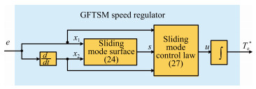 图 3 Block diagram of the designed GFTSM speed regulator.Fig. 3 Block diagram of the designed GFTSM speed regulator.
By solving differential equation (26), the time from any state $s(0)\neq 0$ to the sliding mode surface $s(t_f)$ can be derived as follows:
$ \begin{align} % eq:(28) t_f=\frac{m}{ \varphi(m-v)}\ln\frac{\varphi\left(s(0)\right)^\frac{m-v}{m}+\gamma}{ \gamma}. \end{align} $
(28) Remark 7: From (27), it can be seen that the sliding mode control law does not include switching item and thus weakens system chatter.
Remark 8: Under control law (27), one can easily see that if it converges to zero according to the terminal attractor (26), $x_1$ will accordingly converge to zero in terms of the following fast terminal attractor
$ \begin{align} % eq:(29) \dot{x}_{1}=-\alpha x_{1}-\beta x_{1}^\frac{q}{p}. \end{align} $
(29) It can be observed from (26) and (29) that the fast terminal attractors are adopted both in the reaching phase and in sliding phase. Consequently, the designed regulator (27) is a global terminal sliding mode one which guarantees the finite time control performance.
Remark 9: According to (28), $t_f$ can be set arbitrarily by adjusting parameters $m$, $v$, $\varphi$, $\gamma$.
Remark 10: The designed GFTSM speed regulator (27) is not only stable but also robust, which will be analyzed as below.
3.2.2 Stability Analysis
Construct Lyapunov function as
$ \begin{align} % eq:(30) V_2=\frac{1}{2}s^{2}. \end{align} $
(30) Differentiating (30) yields
$ \dot{V}_2=s\dot{s}=-\varphi s^2-\gamma s^\frac{m+v}{m} $
since $(m+v)$ is an even number, therefore $\dot{V}=s\dot{s}<0$. According to Lyapunov stability theory, the system (23) is stable and its movement can tend to sliding mode surface and finally reach the sliding mode.
3.2.3 Robustness Analysis
Considering parameter uncertainties and external disturbances, the system (23) is rewritten as following:
$\begin{align} % eq:(31) \begin{cases} \dot{x}_{1}=x_2\\[1mm] \dot{x}_{2}=-\dfrac{B_{\rm m}}{ J}x_2-\dfrac{1}{ J}u+d(x_1, x_2) \end{cases} \end{align} $
(31) where $d(x_1, x_2)$ can be regarded as the total disturbance including uncertainties and external disturbances. Assume $| d(x_1, x_2)|$ $\leq$ $D$, $D$ is maximum value.
As for system (31), differentiating (24) yields
$ \begin{align} % eq:(32) \dot{s}=\left(\alpha-\frac{B_{\rm m}}{ J}\right)x_2-\frac{1}{ J}u+d(x_1, x_2)+\beta\frac{{d}}{{d}t}\left(x_{1}^\frac{q}{p}\right). \end{align} $
(32) Substituting (27) into (32) yields
$ \begin{align} % eq:(33) \dot{s}& =-\varphi s-\gamma s^\frac{v}{m}+d(x_1, x_2)\notag\\[1mm] & =-\varphi s-\left(\gamma-\frac{d(x_1, x_2)} {s^\frac{v}{m}}\right)s^\frac{v}{m}. \end{align} $
(33) Let
$ \begin{align} % eq:(34) \bar{\gamma}=\gamma-\frac{d(x_1, x_2)}{s^\frac{v}{m}} \end{align} $
(34) then (33) can be rewritten as
$ \begin{align} % eq:(35) \dot{s}=-\varphi s-\bar{\gamma} s^\frac{v}{m}. \end{align} $
(35) To make (35) be a fast terminal attractor, (34) must satisfy $\bar{\gamma}>0$. Therefore, the following inequality holds true
$ \gamma-\frac{d(x_1, x_2)}{s^\frac{v}{m}}>\gamma-\frac{| d(x_1, x_2)|}{| s^\frac{v}{m}|}>\gamma-\frac{D}{ | s^\frac{v}{m}|}>0 $
then we can deduce
$ \begin{align} % eq:(36) \gamma>\frac{D}{ | s^\frac{v}{m}|}. \end{align} $
(36) Equation (36) is equivalent to
$ \begin{align} % eq:(37) | s|>\left(\frac{D}{ \gamma }\right)^\frac{m}{v}. \end{align} $
(37) As a result, the fast terminal convergence region $\Delta$ is constrained by
$ \begin{align} % eq:(38) \Delta=\left\{x_1, x_2:| s|\leq \left(\frac{D}{ \gamma }\right)^\frac{m}{v}\right\}. \end{align} $
(38) Furthermore, we assume
$ \begin{align} % eq:(39) \gamma={D\over | s^\frac{v}{m}|}+\eta, ~~~\eta>0. \end{align} $
(39) According to (35), the time from any state $s(0)\neq 0$ to the sliding surface is deduced as follows:
$ \begin{align} % eq:(40) \bar{t}_f={m\over \varphi(m-v)}\ln{\varphi\left(s(0)\right)^\frac{m-v}{m}+\bar{\gamma}\over \bar{\gamma}}. \end{align} $
(40) Since $\bar{\gamma}>\eta$, the following inequality can be deduced
$ \ln\frac{\varphi\left(s(0)\right)^\frac{m-v}{m}+\bar{\gamma}}{ \bar{\gamma}}\leq \ln\frac{\varphi\left(s(0)\right)^\frac{m-v}{m}+\eta}{ \eta} $
and then the reaching time satisfies
$ \begin{align} % eq:(41) \bar{t}_f\leq\frac{m}{ \varphi(m-v)}\ln\frac{\varphi\left(s(0)\right)^\frac{m-v}{m}+\eta}{ \eta}. \end{align} $
(41) Through the above analysis, it can be seen that if the condition $\bar{\gamma}>0$ holds then fast terminal convergence can be guaranteed and system (31) can reach neighborhood $\Delta$ of the sliding mode surface $s(\bar{t}_f)=0$ in finite time $\bar{t}_f$.
3.3 Model Predictive Torque Control
The basic idea of MPTC is to predict the future behavior of the variables over a time frame based on the model of the system. As shown in Fig. 1, MPTC includes three parts: cost function minimization, predictive model and flux and torque estimator.
3.3.1 Cost Function Minimization
For MPTC, the cost function is chosen such that both torque and flux at the end of the cycle is as close as possible to the reference value. Generally, the minimum value of cost function is defined as
$ \begin{align} % eq:(42) &\min g =\left| T_{\rm e}^{\ast}-T_{\rm e}^{k+1}\right|+k_3\left| \left| \psi_{\rm s}^{\ast}\right|-| \psi_{\rm s}^{k+1}| \right|\notag \\ &\, {\rm s.t.}\quad u_{\rm s}^{k}\in\{V_1, V_2, \ldots, V_6\} \end{align} $
(42) where $V_1$, $V_2$, $V_3$, $V_4$, $V_5$, and $V_6$ are six nonzero voltage space vectors and can be generated by three phase VSI with respect to the different switches states. A set of voltage space vectors $u_{\rm s}^{k}$ at $k$th instant is defined as
$ \begin{align} % eq:(43) u_{\rm s}^{k}=\frac{2V_{\rm dc}\left[S_{\rm a}^{k}+e^\frac{i2\pi}{3}S_{\rm b}^{k}+(e^\frac{i2\pi}{3})^{2}S_{\rm c}^{k}\right]}{3} \end{align} $
(43) where $S_{\rm a}^{k}~(x=a, b, c)$ at $k$th instant is upper power switch state of one of three legs. $S_{\rm a}^{k}=1$ or $S_{\rm a}^{k}=0$ when upper power switch of one leg is on or off. $k_3$ is the weighting factor.
In order to compensate inherent one-step delay which exists in practical digital system, the cost function (42) is revised as below:
$ \begin{align} % eq:(44) &\min g =\left| T_{\rm e}^{\ast}-T_{\rm e}^{k+2}\right|+k_3\left| \left| \psi_{\rm s}^{\ast}\right|-| \psi_{\rm s}^{k+2}| \right|\notag \\ &\, {\rm s.t.}\quad u_{\rm s}^{k}\in\{V_1, V_2, \ldots, V_6\}. \end{align} $
(44) 3.3.2 Predictive Model for Stator Currents
According to (1), the prediction of the stator current at the next sampling instant is expressed as
$ \begin{align} % eq:(45) \begin{cases} i_{\rm d}^{k+1}=i_{\rm d}^{k}+\dfrac{1}{L}\left(u_{\rm d}^{k}-R_{\rm s}i_{\rm d}^{k}+p\omega_{\rm r}^{k}Li_{\rm q}^{k}\right)T_{\rm s}\\[3mm] i_{\rm q}^{k+1}=i_{\rm q}^{k}+\dfrac{1}{ L}\left (u_{\rm q}^{k}-R_{\rm s}i_{\rm q}^{k}-p\omega_{\rm r}^{k} (Li_{\rm d}^{k}+\psi_{\rm m})\right)T_{\rm s} \end{cases} \end{align} $
(45) where $i_{\rm d}^{k}$, $i_{\rm q}^{k}$ and $R_{\rm s}$ are replaced by the corresponding estimated values coming from the observer in Fig. 2. $T_{\rm s}$ is the sampling period.
3.3.3 Torque and Flux Estimators
In $dq$-frame, the current-based flux-linkage can be expressed as following vector:
$ \begin{align} \left[% eq:(46) \begin{array}{c} \psi_{\rm d}^{k+1} \\ \psi_{\rm q}^{k+1} \\ \end{array} \right]=\left[ \begin{array}{cc} L&0 \\ 0&L \\ \end{array} \right]\left[ \begin{array}{c} i_{\rm d}^{k+1} \\ i_{\rm q}^{k+1}\\ \end{array} \right]+\left[ \begin{array}{c} \psi_{\rm m} \\ 0 \\ \end{array} \right]. \end{align} $
(46) The magnitude of stator flux linkage $\psi_{\rm s}$ is
$ \begin{align} % eq:(47) \psi_{\rm s}^{k+1}=\sqrt{(\psi_{\rm d}^{k+1})^2+(\psi_{\rm q}^{k+1})^2}. \end{align} $
(47) Electromagnetic torque developed in $dq$-frame can be estimated as following:
$ \begin{align} % eq:(48) T_{\rm e}^{k+1}=\frac{3}{ 2}{ p}\psi_{\rm m}i_{\rm q}^{k+1}. \end{align} $
(48) Substituting (45) into (48), the torque can be calculated.
4. Simulation Result and Analysis
In order to validate the effectiveness of proposed control strategy, the designed control system as shown in Fig. 1 has been implemented in MATLAB/Simulink/Simscape platform. The parameters of PMSM drive are given in Table Ⅰ. The sampling period is 100 $\mu$s, and value $k_3$ is selected to be 200. The reference stator flux $\psi_{\rm s}^{\ast}$ is 0.175 Wb. The parameters of the adaptive observer are
$ \begin{align*} &K_{P(R_{\rm s})}=0.006, ~~~K_{I(R_{\rm s})}=8\\ &k_1=30, ~~~k_2=5000, ~~~r=1000. \end{align*} $
表 Ⅰ PARAMETERS OF PMSM DRIVETable Ⅰ PARAMETERS OF PMSM DRIVESymbol Value Symbol Value $R_{\rm s}$ $2.875\, \Omega$ $\omega_{\rm r}^{\ast}$ 1000 rpm $L_{\rm d}, L_{\rm q}$ 0.0085 H $T_{\rm n}$ 4 N$\cdot$m $\psi_{\rm m}$ 0.175 Wb $J$ $0.0008\, {\rm Kg\cdot m}^2$ $p$ 4 $B_{\rm m}$ 0.001 N$\cdot$m$\cdot$s $V_{\rm dc}$ 300 V $T_{\rm f}$ 0 The parameters of GFTSM in Fig. 3 are determined as follows:
$ \begin{align*} &\alpha=100, ~~~\beta=250, ~~~p=7, ~~~q=5\\ &\varphi=1000, ~~~\gamma=80\, 000, ~~~ m=3, ~~~v=1.\end{align*} $
4.1 The GFTSM-based MPTC PMSM Drive System Comparison Between the One With Single Phase Current Sensor and the Other With Two Phase Current Sensors
In order to verify estimation accuracy of the observer for GFTSM-based MPTC PMSM drive system with single phase current sensor, two scenarios of numerical simulation are provided and compared, which correspond to PMSM system with two phase current sensors (phase-$a$ and -$b$ sensors) and PMSM system with single phase current sensor (phase-$b$), respectively. For convenience sake, the former scenario is marked as Case 1 and the latter one as Case 2. Except the above-mentioned different number of current sensors, the two systems employ completely identical GFTSM-based MPTC strategy.
Fig. 4 shows comparison of two scenarios in terms of stator currents, stator resistance, rotor speed and torque when the reference speed $n^{\ast}$ is set to 1000 pm, the load torque is increased from 0 N$\cdot$m to 4 N$\cdot$m at 0.1 seconds and the stator resistance is changed from its nominal value 2.875 $\Omega$ to 5 $\Omega$ at 0.3 seconds.
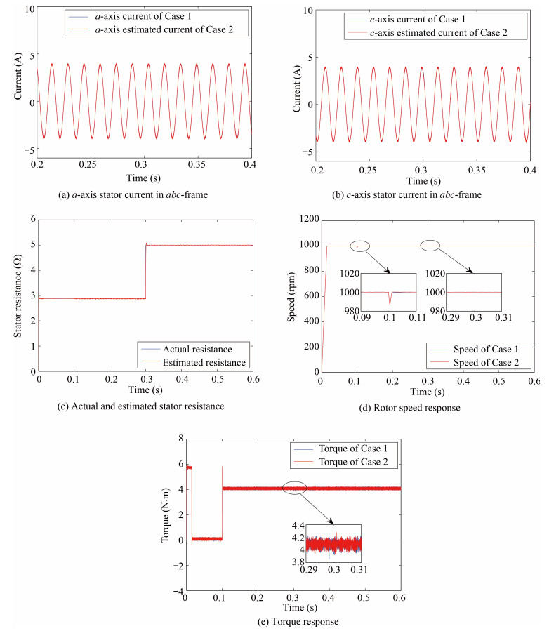 图 4 Dynamic response comparison between Case 1 and Case 2 under the variation of stator resistance.Fig. 4 Dynamic response comparison between Case 1 and Case 2 under the variation of stator resistance.
From Figs. 4(a)$-$4(c), it can be seen that, for designed adaptive observer of Case 2, its estimated $a$-axis and $c$-axis currents in $abc$-frame rapidly track corresponding ones of Case 1, and its estimated stator resistance can rapidly follow actual resistance change and converge to its actual value accurately. Figs. 4(d)$-$4(e) show that, for GFTSM-based MPTC system of Case 2, its speed and torque can be regulated in a satisfactory manner and it has almost as good performance as GFTSM-based MPTC system of Case 1.
4.2 The MPTC PMSM System Comparison Between the One Based on PI and the Other Based on GFTSM
For GFTSM-based MPTC PMSM systems, for the sake of verifying its stronger robustness, two systems are compared, which correspond to the PI-based and GFTSM-based MPTC PMSM systems, respectively. Except distinct outer-loop speed regulator (i.e., PI and GFTSM), the two systems employ completely identical MPTC and adaptive observer. In the simulation, their reference speeds $n^{\ast}$ are set to 1000 rpm, their load torques of 0 N$\cdot$m are increased to 4 N$\cdot$m at 0.1 seconds and stator resistance is at its nominal value 2.875 $\Omega$.
In the simulation, sampling values of three-phase currents are recorded over the time range from 0.1 seconds to 0.2 seconds. During this period, the fundamental frequency of three-phase currents is 66.67 Hz. Total harmonic distortion (THD) can be obtained by comparing the higher frequency components to the fundamental one.
4.2.1 The Comparison of Anti-load Variation Ability Under the Same Speed Transient Response
The parameters of PI for PI-based MPTC PMSM system are adjusted as follows:
$ K_P=0.7, ~~~K_I=0.03 $
such that PI-based MPTC system has almost the same speed transient response as GFTSM-based one.
Fig. 5 shows the dynamical responses in terms of speed, torque and stator currents. Fig. 5(a) intuitively gives the speed response comparison, which demonstrates that for GFTSM-based MPTC PMSM system, its speed can sharply adapt to the change of external load in a satisfactory manner, and its capability of accommodating the challenge of load disturbance is superior to PI-based one's. From Figs. 5(b)$-$5(d), it can be observed that for two systems with same adaptive observer, their torques, estimated $a$-axis and $c$-axis currents in $abc$-frame are almost the same.
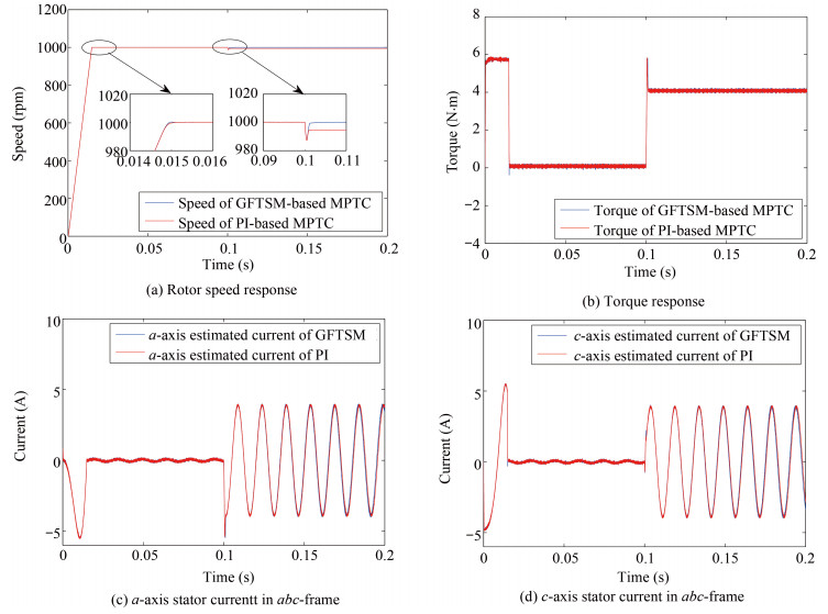 图 5 The comparison of anti-load variation ability under the same speed transient response.Fig. 5 The comparison of anti-load variation ability under the same speed transient response.
Table Ⅱ shows THD comparison of three-phase currents. From Table Ⅱ, what can be observed is that the THD of the GFTSM-based MPTC is smaller than one of the PI-based MPTC.
表 Ⅱ THD OF THREE-PHASE STATORS' CURRENT(%)Table Ⅱ THD OF THREE-PHASE STATORS' CURRENT(%)Control scheme $i_{\rm a}$ $i_{\rm b}$ $i_{\rm c}$ PI-based MPTC $2.21$ $2.32$ $2.24$ GFTSM-based MPTC $1.84$ $1.88$ $1.85$ 4.2.2 The Comparison of Dynamic Responses Under the Same Speed Anti-load Variation Ability
The parameters of PI for PI-based MPTC PMSM system are adjusted as follows:
$ K_P=3, ~~~K_I=0.1 $
such that PI-based MPTC system has almost the same anti-load variation ability as GFTSM-based one.
Figs. 6(a)$-$6(d) show the dynamical responses in terms of speed, torque and stator currents. Fig. 6(a) intuitively gives their speed response comparison, which indicates that GFTSM-based MPTC PMSM system has smaller overshoot and faster settling time than PI-based one. Meanwhile, it can be found from Fig. 6(b) that the torque response of GFTSM-based MPTC PMSM system is better than one of PI-based. From Figs. 6(c)$-$6(d), it can be observed that, their estimated $a$-axis and $c$-axis currents in $abc$-frame are almost the same.
 图 6 The comparison of dynamical response under the same speed anti-load variation ability.Fig. 6 The comparison of dynamical response under the same speed anti-load variation ability.
4.3 The MPTC PMSM System Comparison Between the One Based on SM and the Other Based on GFTSM
Here, the working condition of PMSM drive system is identical with Section 4.2.
For SM-based speed regulator, its sliding mode surface and its reaching law are selected as following:
$ s=ce+\dot{e} $
(49) $ \dot{s}=-k_4s-\varepsilon {\rm sign}(s) $
(50) 4.3.1 The Comparison of Anti-load Variation Ability Under the Same Speed Transient Response
The parameters of SM for SM-based MPTC PMSM system are adjusted as follows:
$ c=160, ~~~k_4=800, ~~~\varepsilon=3\times 10^5 $
such that SM-based MPTC system has almost the same speed transient response as GFTSM-based one.
Figs. 7(a)$-$7(d) show the dynamical responses in terms of speed, torque and stator currents. Fig. 7(a) illustrates that for GFTSM-based MPTC PMSM system, benefiting from the fast terminal sliding mode employed in both the reaching stage and the sliding stage, its recovery rate of speed response is obviously faster than SM-based one. From Figs. 7(b)$-$7(d), it can be seen that for two systems with same adaptive observer, their torques, estimated $a$-axis and $c$-axis currents in $abc$-frame are almost the same.
 图 7 The comparison of anti-load variation ability under the same speed transient response.Fig. 7 The comparison of anti-load variation ability under the same speed transient response.
Table Ⅲ shows THD comparison of three-phase currents. From Table Ⅲ, what can be observed is that the THD of the GFTSM-based MPTC is smaller than one of the SM-based MPTC.
表 Ⅲ THD OF THREE-PHASE STATORS' CURRENT(%)Table Ⅲ THD OF THREE-PHASE STATORS' CURRENT(%)Control scheme $i_{\rm a}$ $i_{\rm b}$ $i_{\rm c}$ SM-based MPTC $2.01$ $2.12$ $2.14$ GFTSM-based MPTC $1.84$ $1.88$ $1.85$ 4.3.2 The Comparison of Dynamic Response Under the Same Speed Anti-load Variation Ability
The parameters of SM for SM-based MPTC PMSM system are adjusted as follows:
$ c=140, ~~k_4=2500, ~~\varepsilon=3\times 10^7 $
such that SM-based MPTC system has almost the same anti-load variation ability as GFTSM-based one.
Figs. 8(a)$-$8(d) show the dynamical responses in terms of speed, torque and stator currents. Fig. 8(a) shows that the speed dynamic performance is better than SM-based one. And it can be found from Figs. 8(b)$-$8(d) that for SM-based MPTC PMSM system, due to a switching function sign$(\cdot)$ in (50), therefore its torque, estimated $a$-axis and $c$-axis currents have significantly heavy chatter. On the other hand, for GFTSM-based one, its sliding reaching law in (26) is a continuous and smooth function, so the system chatter can be greatly reduced.
 图 8 The comparison of dynamic response under the same anti-load variation ability.Fig. 8 The comparison of dynamic response under the same anti-load variation ability.
Summarizing above simulation experiments, we can obtain following results,
1) The proposed adaptive observer can estimate the remaining two phase currents and stator resistance rapidly and accurately.
2) Compared with PI-based and SM-based MPTC PMSM drive systems, GFTSM-based one has better dynamical response behavior and stronger robustness as well as smaller THD index of three-phase stator current.
5. Conclusions
This paper has put forward a novel GFTSM-based MPTC strategy for PMSM drive system with only one phase current sensor. Firstly, an adaptive observer is designed, which is capable of concurrent online estimation of the remaining two phase currents and time-varying stator resistance rapidly and accurately. Secondly, GFTSM speed regulator is designed and its stability and convergence as well as robustness are analytically verified based on Lyapunov stability theory. Finally, the MPTC strategy is employed to reduce the torque and flux ripples. The proposed observer can be embedded into a fault resilient PMSM drive system. In case of a phase current sensor failure, the designed observer can be used as a virtual current sensor which is robust against variation of stator resistance. And the designed GFTSM controller can enhance speed regulator's robustness against variation of system parameters and external disturbance. The resultant GFTSM-based MPTC strategy can guarantee that PMSM drive system with single phase current sensor achieves not only fast response but also high-precision control performance as well as strong robustness.
Our future research topic is that considering both parameters uncertainties and unmodeled dynamics, we will employ adaptive robust method with extended state observer to reconstruct stator currents observer.
-
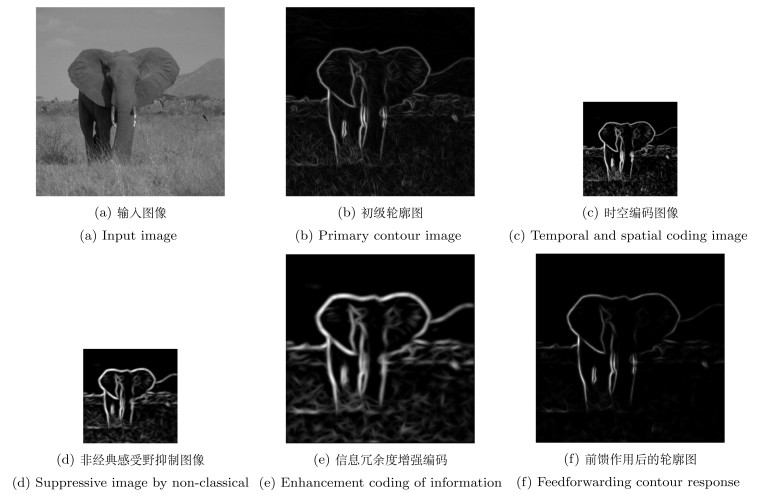
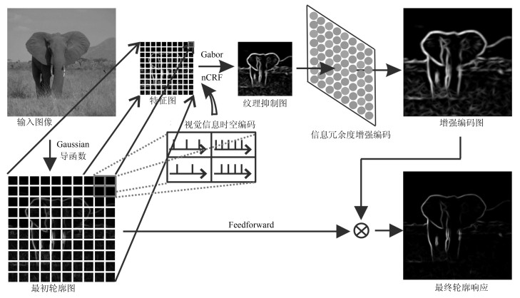
图 3 视通路神经编码及前馈融合示意图
Fig. 3 Schematic diagram of visual pathway with neural coding and feedforward fusion

图 4 RuG40图库中的轮廓测试结果(第1行为用于测试的自然场景图; 第2行为基准轮廓图; 第3行为GD检测结果; 第4行为CORF检测结果; 第5行为ISO检测结果; 第6行为MCI检测结果; 第7行为ISSC检测结果; 第8行为NNC检测结果; 第9行为MNC检测结果)
Fig. 4 Contour test results of the RuG40 gallery (The first line is the input of natural scene images; The second line is the contour baselines; The third line is the results of GD; The fourth line is the results of CORF; The fifth line is the results of ISO; The sixth line is the results of MCI; The seventh line is the results of ISSC; The eighth line is the results of NNC; The ninth line is the results of MNC)

图 5 各模型在整个数据集中的定量分析图
Fig. 5 Quantitative comparison of various models on the whole RuG40 dataset

图 6 随机选取的6组图像在多组参数下检测结果的$P$值盒须图统计(I表示ISO方法, C表示MCI方法, S表示ISSC方法, N表示NNC方法, M表示MNC方法)
Fig. 6 Box-and-Whisker plots of the performance of the ISO (denoted by I), the MCI (denoted by C), the ISSC (denoted by S), the NNC (denoted by N), and the MNC (denoted by M) for six random test images of multiparameters
表 1 图 4中不同方法的参数设置, 性能指标及运行速度.
Table 1 Parameters, speed and performance of the different methods in Fig. 4
图像 算法 $\alpha$ $p$ ${e_{FP}}$ ${e_{FN}}$ $P$ $\rm FPS$ GD 0.20 1.50 0.13 0.30 4 CORF 0.20 0.42 0.30 0.50 3/5 ISO 0.80 0.20 0.25 0.38 0.55 3 buffalo MCI 0.70 0.30 0.18 0.29 0.59 1/22 ISSC 0.10 0.22 0.27 0.58 1/8 NNC 0.20 0.10 0.22 0.32 0.54 1 MNC 0.10 0.30 0.21 0.27 0.64 1/2 GD 0.10 1.29 0.25 0.39 CORF 0.20 0.32 0.29 0.52 ISO 1.00 0.10 0.37 0.32 0.53 elephant 2 MCI 0.40 0.30 0.22 0.30 0.58 ISSC 0.10 0.25 0.30 0.56 NNC 0.20 0.30 0.28 0.30 0.56 MNC 0.10 0.20 0.13 0.36 0.62 GD 0.25 1.33 0.18 0.45 CORF 0.20 0.41 0.29 0.50 ISO 0.60 0.20 0.29 0.27 0.58 golf cart MCI 0.90 0.40 0.23 0.28 0.62 ISSC 0.3 0.30 0.30 0.55 NNC 0.10 0.30 0.27 0.29 0.57 MNC 0.10 0.40 0.26 0.24 0.62 GD 0.25 1.33 0.18 0.45 CORF 0.30 0.55 0.14 0.58 ISO 0.90 0.10 0.21 0.27 0.61 hyena MCI 0.60 0.50 0.19 0.22 0.65 ISSC 0.20 0.28 0.24 0.59 NNC 0.20 0.20 0.30 0.24 0.59 MNC 0.10 0.20 0.21 0.27 0.64 GD 0.20 1.77 0.15 0.25 CORF 0.30 0.67 0.32 0.45 ISO 0.80 0.20 0.32 0.51 0.47 lions MCI 1.00 0.50 0.48 0.29 0.50 ISSC 0.3 0.45 0.30 0.48 NNC 0.30 0.30 0.45 0.31 0.47 MNC 0.70 0.40 0.45 0.28 0.51  下载: 导出CSV
-
[1] Mignotte M. A biologically inspired framework for contour detection. Pattern Analysis and Applications, 2017, 20(2): 365-381 doi: 10.1007/s10044-015-0494-y [2] Ding L J, Goshtasby A. On the Canny edge detector. Pattern Recognition, 2001, 34(3): 721-725 doi: 10.1016/S0031-3203(00)00023-6 [3] 蒋朝辉, 吴巧群, 桂卫华, 阳春华, 谢永芳.基于分数阶的多向微分算子的高炉料面轮廓自适应检测.自动化学报, 2017, 43(12): 2115-2126 doi: 10.16383/j.aas.2017.c160621Jiang Zhao-Hui, Wu Qiao-Qun, Gui Wei-Hua, Yang Chun-Hua, Xie Yong-Fang. Adaptive detection of blast furnace surface contour with fractional multi-directional differential operator. Acta Automatica Sinica, 2017, 43(12): 2115-2126 doi: 10.16383/j.aas.2017.c160621 [4] Arbelaez P, Maire M, Fowlkes C, Malik J. Contour detection and hierarchical image segmentation. IEEE Transactions on Pattern Analysis and Machine Intelligence, 2011, 33(5): 898-916 doi: 10.1109/TPAMI.2010.161 [5] Martin D R, Fowlkes C C, Malik J. Learning to detect natural image boundaries using local brightness, color, and texture cues. IEEE Transactions on Pattern Analysis and Machine Intelligence, 2004, 26(5): 530-549 doi: 10.1109/TPAMI.2004.1273918 [6] Young R A, Lesperance R M. The Gaussian derivative model for spatial-temporal vision: II. Cortical data. Spatial Vision, 2001, 14(3): 321-389 [7] Azzopardi G, Petkov N. A CORF computational model of a simple cell that relies on LGN input outperforms the Gabor function model. Biological Cybernetics, 2012, 106(3): 177-189 doi: 10.1007/s00422-012-0486-6 [8] Grigorescu C, Petkov N, Westenberg M A. Contour detection based on nonclassical receptive field inhibition. IEEE Transactions on Image Processing, 2003, 12(7): 729-739 doi: 10.1109/TIP.2003.814250 [9] Zeng C, Li Y J, Li C Y. Center-surround interaction with adaptive inhibition: a computational model for contour detection. NeuroImage, 2011, 55(1): 49-66 doi: 10.1016/j.neuroimage.2010.11.067 [10] Yang K F, Li C Y, Li Y J. Multifeature-based surround inhibition improves contour detection in natural images. IEEE Transactions on Image Processing, 2014, 23(12): 5020-5032 doi: 10.1109/TIP.2014.2361210 [11] 廖进文, 范影乐, 武薇, 高云园, 李轶.基于抑制性突触多层神经元群放电编码的图像边缘检测.中国生物医学工程学报, 2014, 33(5): 513-524 doi: 10.3969/j.issn.0258-8021.2014.05.01Liao Jin-Wen, Fan Ying-Le, Wu Wei, Gao Yun-Yuan, Li Yi. Image edge detection based on spike coding of multilayer neuronal population with inhibitory synapse. Chinese Journal of Biomedical Engineering, 2014, 33(5): 513-524 doi: 10.3969/j.issn.0258-8021.2014.05.01 [12] Chen M G, Yan Y, Gong X J, Gilbert C D, Liang H L, Li W. Incremental integration of global contours through interplay between visual cortical areas. Neuron, 2014, 82(3): 682-694 doi: 10.1016/j.neuron.2014.03.023 [13] Freud E, Plaut D C, Behrmann M. `What' is happening in the dorsal visual pathway. Trends in Cognitive Sciences, 2016, 20(10): 773-784 doi: 10.1016/j.tics.2016.08.003 [14] Taylor W R, Vaney D I. Diverse synaptic mechanisms generate direction selectivity in the rabbit retina. The Journal of Neuroscience, 2002, 22(17): 7712-7720 doi: 10.1523/JNEUROSCI.22-17-07712.2002 [15] Bays P M. A signature of neural coding at human perceptual limits. Journal of Vision, 2016, 16(11): 4 doi: 10.1167/16.11.4 [16] Zhu M C, Rozell C J. Visual nonclassical receptive field effects emerge from sparse coding in a dynamical system. PLoS Computational Biology, 2013, 9(8): e1003191 doi: 10.1371/journal.pcbi.1003191 [17] Yu Q, Tang H J, Tan K C, Li H Z. Rapid feedforward computation by temporal encoding and learning with spiking neurons. IEEE Transactions on Neural Networks and Learning Systems, 2013, 24(10): 1539-1552 doi: 10.1109/TNNLS.2013.2245677 [18] Hu J, Tang H J, Tan K C, Li H Z. How the brain formulates memory: a spatio-temporal model research frontier. IEEE Computational Intelligence Magazine, 2016, 11(2): 56-68 doi: 10.1109/MCI.2016.2532268 [19] Buonocore A, Caputo L, Pirozzi E, Carfora M F. A leaky integrate-and-fire model with adaptation for the generation of a spike train. Mathematical Biosciences and Engineering, 2016, 13(3): 483-493 doi: 10.3934/mbe.2016002 [20] Muhle-Karbe P S, Duncan J, De Baene W, Mitchell D J, Brass M. Neural coding for instruction-based task sets in human frontoparietal and visual cortex. Cerebral Cortex, 2017, 27(3): 1891-1905 http://www.wanfangdata.com.cn/details/detail.do?_type=perio&id=9ed89e2bff4ffeffe9386fd3452382c7 [21] Tang J Y, Jimenez S C A, Chakraborty S, Schultz S R. Visual receptive field properties of neurons in the mouse lateral geniculate nucleus. PLoS One, 2016, 11(1): e0146017 doi: 10.1371/journal.pone.0146017 [22] 谢昭, 童昊浩, 孙永宣, 吴克伟.一种仿生物视觉感知的视频轮廓检测方法.自动化学报, 2015, 41(10): 1814-1824 doi: 10.16383/j.aas.2015.c150018Xie Zhao, Tong Hao-Hao, Sun Yong-Xuan, Wu Ke-Wei. Dynamic contour detection inspired by biological visual perception. Acta Automatica Sinica, 2015, 41(10): 1814-1824 doi: 10.16383/j.aas.2015.c150018 [23] 李智勇, 何霜, 刘俊敏, 李仁发.基于蛙眼R3细胞感受野模型的运动滤波方法.自动化学报, 2015, 41(5): 981-990 doi: 10.16383/j.aas.2015.c140810Li Zhi-Yong, He Shuang, Liu Jun-Min, Li Ren-Fa. Motion filtering by modelling R3 cell's receptive field in frog eyes. Acta Automatica Sinica, 2015, 41(5): 981-990 doi: 10.16383/j.aas.2015.c140810 -

 下载:
下载:
计量
- 文章访问数: 1686
- HTML全文浏览量: 438
- PDF下载量: 219
- 被引次数: 0
