

-
摘要: 作为表征控制系统故障诊断能力的属性, 故障可诊断性揭示了故障诊断深层次的内涵.将可诊断性分析纳入控制系统与诊断方案的设计环节, 可以从根本上提高系统对故障的诊断能力, 为研究故障诊断提供新的思路.本文分别从可诊断性的内涵、研究现状以及潜在发展趋势三个角度系统地对可诊断性进行分析.首先, 从定义、影响因素、与已有概念的关系以及应用四个方面剖析了控制系统可诊断性的内涵和研究意义.其次, 分别从可诊断性评价与设计两个方面对可诊断性的研究现状进行分析.最后, 通过对可诊断性已有成果进行总结归纳, 探讨了可诊断性研究存在的不足以及未来发展的趋势.Abstract: As a property describing fault diagnosis ability of control systems, diagnosability reveals deep insight into fault diagnosis.The fault diagnosis ability can be fundamentally improved by incorporating diagnosability analysis into the designs of control systems and diagnosis programs, which provides a new way for the study of fault diagnosis.To systematically analyze the diagnosability, the connotations, research status and potential research tendencies of diagnosability are discussed.First of all, the concept and research significance of diagnosability are summarized from four sides, definition, influence factors, relationships between diagnosability and other concepts, and applications.Moreover, the current research status of diagnosability is discussed in terms of diagnosability evaluation and design.Finally, the deficiency and prospects of diagnosability study are predicated based on existing results.
-
1. Introduction
For permanent magnet synchronous motor (PMSM) drive system, the measurement of instantaneous stator currents is required for successful operation of the feedback control. Generally two phase current sensors are installed in three phase voltage source inverters (VSI). Nevertheless, sudden severe failure of phase current sensors would result in over-current malfunction of the drive system. And if there is no protection scheme in the gate-drive circuit, the failure would lead to irrecoverable fault of power semiconductors in VSI, which would cause degradation of motor drive performance. Additionally, some minor failures (such as gain drift and nonzero offset) of phase current sensors would lead to torque pulsation synchronizing with the inverter output frequency [1]. The larger offset and scaling error of phase current sensors would bring about the worse performance of torque regulation. Moreover, if the offset and gain drift are above certain level, it would cause over-current trip under high speed and heavy load conditions [2]. So it is necessary to consider fault tolerant operation of phase current sensor failure.
The current sensorless technology, regarded as fault tolerant one, has been developed in the past few decades. Its core lies in that the physical fault current sensor is replaced with virtual sensor (or current estimator). This technology has several advantages such as high reliability and low cost as well as space and weight savings owing to omitting physical current sensor. Moreover, it allows the drive system to work in hostile environment.
As far as the current sensorless technique is concerned, three estimation solutions have been reported in the literature. The first one is a DC-link current-based approach which restructures phase currents with the information of the DC-link current and switching states in VSI [3]. Although it is a mainstream method, its unavoidable drawbacks are exposed: the duration of an active switching state may be so short that the DC-link current cannot be measured on one hand, on the other hand, there are immeasurable regions in the output voltage hexagon where the DC-link current sampling and reconstruction are limited or impossible to do [4]. In addition, the DC-link sensed current remains sensitive to the narrow pulse and further deteriorates if the cable capacitance causes spurious oscillations in the DC-link waveform. In order to provide high-accuracy phase current reconstruction over a wide range of operating conditions with a low current waveform, over the past years, many kinds of methods of improved PWM modulation strategy have been proposed for the single DC-link current sensor technique [5]$-$[14]. Although many improved methods show reasonable phase current reconstruction performance, these methods suffer from complicated algorithms [15]. The second one is an analytical model-based approach. In [16], on the basis of the voltage and flux equations of induction motor (IM) drive, the phase current is estimated by using the synchronous reference frame variables under single phase current sensor condition. In [17], by the discrete voltage equations of PMSM drive, the phase currents are estimated. Although it is easier to implement than the first one, the method is not robust against the variation of system parameters. The third one is an adaptive observer-based approach. In [18], the phase current is reconfigured for IM drive using single phase current sensor, while in [19], the phase currents are reconfigured for PMSM drive without any phase current sensors. Compared with the first two solutions, the third solution has stronger robustness against the variation of system parameters [20], [21]. For PMSM drive system when only one phase current sensor is available, the remaining two phase currents estimation based on an adaptive observer must be studied, which is required to perform current feedback control. However, there is no literature on such strategy.
For PMSM drive system, model predictive torque control (MPTC) is an emerging control strategy [22]$-$[29]. Its main objective is to control instantaneous torque and stator flux with high accuracy and thus MPTC plays an important role to ensure the quality of the torque and speed control. MPTC adopts the principle of model predictive control (MPC) and can provide high dynamic performance and low stator current harmonics.
For conventional proportional-integral(PI)-based MPTC PMSM drive system, its speed regulator employs the algorithm of PI. In general, PI may perform well under certain operating condition, but it does not work properly and thus degrades dynamic performance under other operating conditions such as variation of system parameters and external disturbances. To improve the robustness of the speed regulator, some techniques have been proposed in recent years [30]$-$[34]. Except these techniques, a global fast terminal sliding mode (GFTSM) control is an effective and practical one [35], [36], which is based on sliding mode theory and employs the fast terminal sliding mode in both the reaching stage and sliding stage. By adding the nonlinear function to the sliding mode surface, the GFTSM controller can enable drive system not only to be superiorly robust against system uncertainties and external disturbances but also to have quick response as well as high control precision. Even so, studies on GFTSM speed regulator are very few. In this paper, we propose replacement of PI with GFTSM for MPTC PMSM drive system.
In this paper, by referring to the adaptive approach and integrating the GFTSM method, a new GFTSM-based MPTC strategy with the adaptive observer is put forward for the PMSM drive system with single phase current sensor. The proposed adaptive observer presents a satisfactory tracking performance of the remaining two phase currents in the presence of stator resistance change caused by the temperature variation. And the designed GFTSM controller enhances the speed regulator's robustness against parameter uncertainty and external disturbance. On the basis of the above foundation, the synthesized MPTC PMSM drive control system achieves a high performance.
This paper is organized as follows: Dynamic model of PMSM drive is presented in Section 2. Section 3 gives the adaptive observer and GFTSM speed regulator design as well as MPTC design. Experimental results and analysis are presented in Section 4. Section 5 contains the conclusions.
Notation 1: The following nomenclature is used throughout this paper:
$ \begin{align*} \begin{array}{lll} R_{\rm s}:& &\mbox {Nominal phase resistance} \ \\ \psi_{\rm m}:&&\mbox{The permanent magnet flux} \ \\ \psi_{\rm s}:&&\mbox{Stator flux linkage}\\ p:&&\mbox{Number of pole pairs}\\ V_{\rm dc}:&&\mbox{DC bus voltage}\\ \omega_{\rm r}:&&\mbox{Rotor actual mechanical speed}\\ T_{\rm l}:&&\mbox{Load torque}\\ T_{\rm e}:&&\mbox{Electromagnetic torque}\\ J:&&\mbox{Moment of inertia}\\ B_{\rm m}:&&\mbox{Viscous friction coefficient}\\ T_{\rm f}:&&\mbox{Coulomb friction torque}\\ \theta:&&\mbox{Rotor electrical angular position}\\ i:&&\mbox{Stator current}\\ u:&&\mbox{Stator voltage}\\ L:&&\mbox{Stator inductance}.\\ \end{array} \end{align*} $
Notation 2: The following symbol is used throughout this paper. $\bullet_{\rm d}$, $\bullet_{\rm q}$, $\bullet_{\alpha}$ and $\bullet_{\beta}$ are used to denote the $d$-axis, $q$-axis, $\alpha$-axis, and $\beta$-axis component of $\bullet$, respectively; $\bullet^{\ast}$ is used to denote the reference values of $\bullet$; $\hat{\bullet}$ is used to denote the estimate of $\bullet$; $\tilde{\bullet}$ is used to denote the parameter estimation error of $\bullet$; $\bullet^{k}$ and $\bullet^{k+1}$ are used to denote the instantaneous value at $k$th and ($k+1$)th of $\bullet$, respectively.
2. Dynamic Models of Three-phase PMSM Drive
As for three-phase PMSM drive, the models in rotor synchronous reference frame ($dq$-frame) and two-phase stationary reference frame ($\alpha\beta$-frame) are expressed as follows, respectively:
$ \begin{align} \label{eq:1} % eq:(1) \begin{cases} \dfrac{{d}i_{\rm d}}{{d}t}&=\dfrac{1}{L_{\rm d}} \left(u_{\rm d}-R_{\rm s}i_{\rm d}+p\omega_{\rm r}L_{\rm q}i_{\rm q}\right) \\[3mm] \dfrac{{d}i_{\rm q}}{{d}t}&=\dfrac{1}{L_{\rm q}}\left(u_{\rm q}-R_{\rm s}i_{\rm q}+p\omega_{\rm r} (L_{\rm d}i_{\rm d}+\psi_{\rm m})\right) \end{cases}\end{align} $
(1) $\begin{align} \begin{cases} \dfrac{{d}i_{\alpha}}{{d}t}&=\dfrac{1}{L_{\alpha}} \left(u_{\alpha}-R_{\rm s}i_{\alpha}+p\omega_{\rm r}\psi_{\rm m} \sin\theta\right) \\[3mm] \dfrac{{d}i_{\beta}}{{d}t}&=\dfrac{1}{L_{\beta}} \left(u_{\beta}-R_{\rm s}i_{\beta}-p\omega_{\rm r}\psi_{\rm m}\cos\theta\right) \end{cases} \end{align} $
(2) and the mechanical equation is expressed as
$ \begin{align} \dfrac{{d}\omega_{\rm r}}{{d}t}=\dfrac{1}{J}(T_{\rm e}-T_{\rm l}-B_{\rm m}\omega_{\rm r}-T_{\rm f}) \end{align} $
(3) where the electromagnetic torque $T_{\rm e}$ is expressed as
$\begin{align} T_{\rm e}=\frac{3{ p}}{2} \left[\psi_{\rm m}i_{\rm q}+(L_{\rm d}-L_{\rm q})i_{\rm d}i_{\rm q}\right]. \end{align} $
(4) 3. Design of GFTSM-based MPTC PMSM Drive System With Adaptive Observer
The objective of GFTSM-based MPTC using adaptive observer is that the PMSM drive system can work reliably and its speed and torque can be controlled not only to have satisfactory performance but also to be strongly robust against parameters variation and external disturbance. The schematic of the proposed control system is shown in Fig. 1. Our design task concentrates on adaptive observer, GFTSM speed regulator and MPTC as follows.
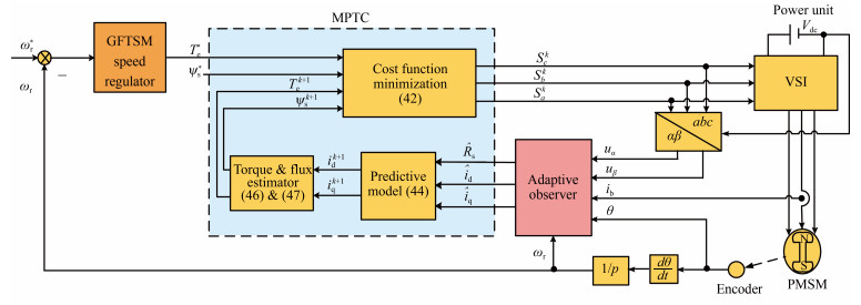 图 1 Block diagram of GFTSM-based MPTC PMSM drive system with adaptive observer.Fig. 1 Block diagram of GFTSM-based MPTC PMSM drive system with adaptive observer.
3.1 Adaptive Observer Design
The proposed adaptive observer is to estimate the remaining two phase currents and stator resistance when single phase current sensor is available. In the design process, assume the following conditions.
1) Only phase-$b$ current can be measured and the remaining two phase current sensors are not available.
2) Due to heating during operating of the motor, the stator resistance $R_{\rm s}$ is considered as a time-varying parameter.
3) There is no saturation in the magnetic circuit.
For surface-mounted PMSM drive, $L_{\rm d}=L_{\rm q}=L_{\alpha}= L_{\beta}$ $=$ $L$. The $\alpha$-axis in $\alpha\beta$-frame is oriented along phase-$a$ axis in three-phase stationary reference frame ($abc$-frame). The $abc$-axis stator currents in $abc$-frame can be obtained from the $\alpha\beta$-axis ones in $\alpha\beta$-frame by the following transformation matrix:
$ \left[ \begin{matrix} {{i}_{\rm{a}}} \\ {{i}_{\rm{b}}} \\ {{i}_{\rm{c}}} \\ \end{matrix} \right]=\left[ \begin{matrix} 1 & 0 \\ -\frac{1}{2} & \frac{\sqrt{3}}{2} \\ -\frac{1}{2} & -\frac{\sqrt{3}}{2} \\ \end{matrix} \right]\left[ \begin{matrix} {{i}_{\alpha }} \\ {{i}_{\beta }} \\ \end{matrix} \right] $
(5) where $i_{\rm a}$, $i_{\rm b}$, and $i_{\rm c}$ are $abc$-axis stator currents in $abc$-frame. From (5), the following equation can be given,
$ \begin{align} % eq:(6) i_{\rm b}=-\frac{1}{2} i_\alpha+\frac{\sqrt{3}}{2}i_\beta. \end{align} $
(6) Taking (2) into account, the time derivative of (6) is deduced as follows:
$ \begin{align} % eq:(7) \frac{{d}i_{\rm b}}{{d}t}& =\dfrac{\sqrt{3}}{2L}\left[u_\beta-R_{\rm s}\left(\frac{1}{ \sqrt{3}}i_\alpha+\frac{2}{ \sqrt{3}}i_{\rm b}\right)-p\omega_{\rm r}\psi_m\cos\theta\right]\notag\\ & \quad -\frac{1}{2L} (u_{\alpha}-R_{\rm s}i_{\alpha}+p\omega_{\rm r}\psi_{\rm m}\sin\theta)\notag\\ &=\frac{\sqrt{3}u_\beta-u_{\alpha}-2R_{\rm s}i_{\rm b}-p\omega_{\rm r}\psi_{\rm m}(\sqrt{3}\cos\theta+\sin\theta)} {2L}. \end{align} $
(7) The following adaptive observer is proposed in order to estimate phase-$b$ current,
$ \begin{align} % eq:(8) \frac{{d}\hat{i}_{\rm b}}{{d}t}& =\frac{\sqrt{3}}{ 2L}\left[u_\beta-\hat{R}_{\rm s}\left(\frac{1}{ \sqrt{3}}\hat{i}_\alpha+\frac{2}{ \sqrt{3}}i_{\rm b}\right)-p\omega_{\rm r}\psi_m\cos\theta\right]\notag\\ & \quad -\frac{1}{ 2L}\left(u_{\alpha}-\hat{R}_{\rm s}\hat{i}_{\alpha}+p\omega_{\rm r}\psi_{\rm m}\sin\theta\right)-k_1f(\tilde{i}_{\rm b})-k_2\tilde{i}_{\rm b}\notag\\ & =\frac{1}{2L}\left[\sqrt{3}u_\beta-u_{\alpha}-2\hat{R}_{\rm s}i_{\rm b}-p\omega_{\rm r}\psi_{\rm m}(\sqrt{3}\cos\theta + \sin\theta)\right]\notag\\ &\quad-k_1f(\tilde{i}_{\rm b})-k_2\tilde{i}_{\rm b} \end{align} $
(8) where $k_1f(\tilde{i}_{\rm b})$ and $k_2\tilde{i}_{\rm b}$ are correctors, and $k_1$ and $k_2$ are the positive observer gains, and $f(\cdot)$ denotes the nonlinear function of phase-$b$ current estimation error $\tilde{i}_{\rm b}$, which is defined as
$ \begin{align} % eq:(9) \tilde{i}_{\rm b}=\hat{i}_{\rm b}-i_{\rm b}. \end{align} $
(9) Define the following stator resistance estimation error,
$ \begin{align} % eq:(10) \tilde{R}_{\rm s}=\hat{R}_{\rm s}-R_{\rm s}. \end{align} $
(10) By subtracting (8) from (7), the dynamics equation of the phase-$b$ current estimation error is given as follows:
$ \begin{align} % eq:(11) \frac{{d}\tilde{i}_{\rm b}}{{d}t}=-\frac{1}{ L}\tilde{R}_{\rm s}i_{\rm b}-k_1f(\tilde{i}_{\rm b})-k_2\tilde{i}_{\rm b}. \end{align} $
(11) In order to determine the adaptive law of the stator resistance and the observer gains, construct the candidate Lyapunov function as
$ \begin{align} % eq:(12) V_1=\frac{1}{ 2}\left(\tilde{i}_{\rm b}^2+{1\over r}\tilde{R}_{\rm s}^2\right) \end{align} $
(12) where $r$ is constant positive scalar.
The time derivative of (12) is obtained as follows:
$ \begin{align} % eq:(13) \frac{{d}{V_1}}{{d}t}=-k_2\tilde{i}_{\rm b}^2-k_1f(\tilde{i}_{\rm b})\tilde{i}_{\rm b}+\tilde{R}_{\rm s}\left(\frac{1}{ r}\frac{{d}\tilde{R}_{\rm s}}{{d}t}-\frac{1}{ L}i_{\rm b}\tilde{i}_{\rm b}\right). \end{align} $
(13) If we define following equality,
$ \begin{align} % eq:(14) \frac{1}{r}\frac{{d}\tilde{R}_{\rm s}}{{d}t}-\frac{1}{ L}i_{\rm b}\tilde{i}_{\rm b}=0. \end{align} $
(14) Equation (13) can be rewritten as below:
$ \begin{align} % eq:(15) \frac{{d}{V_1}}{{d}t}=-k_2\tilde{i}_{\rm b}^2-k_1f(\tilde{i}_{\rm b})\tilde{i}_{\rm b}. \end{align} $
(15) To render $\dot V_{1}$ negative, we assume
$ \begin{align} % eq:(16) f(\tilde{i}_{\rm b})={\rm sign}(\tilde{i}_{\rm b}). \end{align} $
(16) As a result, the following inequality is satisfied
$ \frac{{d}{V_1}}{{d}t}<0. $
By Lyapunov stability theorem, dynamic system (11) is stable, which means that both $\tilde{i}_{\rm b}$ and $\tilde{R}_{\rm s}$ can converge to zero. Since the variation of the stator resistance in the observer time scale is negligible, i.e.,
$ \frac{{d}R_{\rm s}}{{d}t}\approx 0 $
then the following formula holds
$ \begin{align} % eq:(17) \frac{{d}\tilde{R}_{\rm s}}{{d}t}=\frac{{d}\hat{R}_{\rm s}}{{d}t}-\frac{{d}R_{\rm s}}{{d}t}\approx\frac{{d}\hat{R}_{\rm s}}{{d}t}. \end{align} $
(17) Therefore, from (14), the adaptive mechanism of the stator resistance is derived as follows:
$ \begin{align} % eq:(18) \hat{R}_{\rm s}={r\over L}\int(i_{\rm b}\tilde{i}_{\rm b}){ d}t. \end{align} $
(18) With the adaptive mechanism in (18), the estimation value of the stator resistance can converge to its real value.
In order to improve the estimation accuracy of the stator resistance and to ensure a null steady error, on the basis of PI strategy, (18) is modified as below:
$ \begin{align} % eq:(19) \hat{R}_{\rm s}=\frac{r}{ L}\left\{{K_{P(R_{\rm s})}[i_{\rm b}(\hat{i}_{\rm b}-i_{\rm b})]+K_{I(R_{\rm s})}\int[i_{\rm b}(\hat{i}_{\rm b}-i_{\rm b})]{d}t}\right\} \end{align} $
(19) where $K_{P(R_{\rm s})}$ and $K_{I(R_{\rm s})}$ are proportional and integral scalars, respectively.
By replacing $R_{\rm s}$ in (2) with $\hat{R}_{\rm s}$ in (19), the $\alpha\beta$-axis currents observers can be constructed as follows:
$ \begin{align} % eq:(20) \begin{cases} \dfrac{{d}\hat{i}_{\alpha}}{{d}t}=\dfrac{1}{ L} \left(u_{\alpha}-\hat{R}_{\rm s}\hat{i}_{\alpha}+p\omega_{\rm r} \psi_{\rm m}\sin\theta\right) \\[3mm] \dfrac{{d}\hat{i}_{\beta}}{{d}t} =\dfrac{1}{ L}\left(u_{\beta}-\hat{R}_{\rm s}\hat{i}_{\beta} -p\omega_{\rm r}\psi_{\rm m}\cos\theta\right). \end{cases} \end{align} $
(20) By combining (8), (19) and (20), the block diagram of the designed adaptive observer is established as shown in Fig. 2, which treats the stator voltages, rotor electrical position and speed as the inputs, the $dq$-axis currents and stator resistance as outputs when only phase-$b$ current is measured.
 图 2 Block diagram of the proposed adaptive observer.Fig. 2 Block diagram of the proposed adaptive observer.
Remark 1: From Fig. 2, it can be seen that estimating the phase-$b$ current is a key step and primary premise in construction of the adaptive observer. The error between the phase-$b$ measured current and its estimated value must be guaranteed to converge towards zero.
Remark 2: From (8) and (19), it can be seen that although the coupling relationship between $\hat{i}_{\rm b}$ and $\hat{R}_{\rm s}$ exists, we do not need to decouple them in the design process. In fact, the phase-$b$ current estimation (8) and the stator resistance adaptive law (19) are implemented and solved all together.
Remark 3: The convergence rate of the observer is dependent on the observer gains $k_1$ and $k_2$, which should be chosen to be large enough such that the observer responds as soon as possible.
Remark 4: The estimated $dq$-axis currents in Fig. 2 will be applied to MPTC as shown in Fig. 1.
Remark 5: From (5), the estimation of phase-$a$ current in $abc$-frame is equal to that of $\alpha$-axis current in $\alpha\beta$-frame as follows:
$ \begin{align} % eq:(21) \hat{i}_{\rm a}=\hat{i}_{\alpha}. \end{align} $
(21) Accordingly, the estimation of phase-$c$ current in $abc$-frame can be obtained as follows:
$ \hat{i}_{\rm c}=-(i_{\rm b}+\hat{i}_{\alpha}). $
Remark 6: The proposed adaptive observer is robust against only the stator resistance change. If other parameter uncertainties (such as stator inductance change and permanent magnet flux change, etc.) and unmodeled dynamics are required to be considered, then adaptive robust method with extended state observer can be borrowed from [20] and [33], which is our next research topic.
3.2 GFTSM Speed Regulator Design
3.2.1 GFTSM Design
Define the speed error as
$ e=\omega_{\rm r}^{\ast}-\omega_{\rm r}. $
Let
$ \begin{align} % eq:(22) x_1=e, ~~x_2=\dot{x}_{1}, ~~ u=\dot{T}_{\rm e}. \end{align} $
(22) Assume that $\omega_{\rm r}^{\ast}$ (or $\dot{\omega}_{\rm r}^{\ast}$), $T_{\rm l}$, $T_{\rm f}$ are constants and $\omega_{\rm r}$ has continuous second-order derivative. Then, the state equation of (3) can be expressed as following:
$ \begin{align} % eq:(23) \begin{cases} \dot{x}_{1}=x_2\\[1mm] \dot{x}_{2}=-\dfrac{B_{\rm m}}{ J}x_2-\dfrac{1}{ J}u \end{cases} \end{align} $
(23) where $u$ can be regarded as the control input.
Our target is to enable the drive system to be strongly robust and to have very fast response. For this reason, based on sliding mode theory, GFTSM speed regulator is employed. Fast terminal sliding mode surface is designed as following:
$ \begin{align} % eq:(24) s=\dot{x}_{1}+\alpha x_{1}+\beta x_{1}^\frac{q}{p} \end{align} $
(24) where $\alpha$, $\beta>0$; $q$, $p$ $(q<p)$ are positive odd integers.
Taking the first-order derivative of (24) yields
$ \begin{align} % eq:(25) \dot{s}=\left(\alpha-\frac{B_{\rm m}}{ J}\right)x_2-{\frac{1}{ J}}u+\beta\frac{{d}}{{d}t}\left(x_{1}^\frac{q}{p}\right). \end{align} $
(25) To make the system (23) reach the sliding mode surface in finite time, the fast terminal attractor is adopted as follows:
$ \begin{align} % eq:(26) \dot{s}=-\varphi s-\gamma s^\frac{v}{m} \end{align} $
(26) where $\varphi>0$, $\gamma>0$, $m>0$, $v>0$; $m$ and $v$ are odd integers.
Let (25) be equal to (26) and thus the following sliding mode control law can be obtained
$ \begin{align} % eq:(27) u=J\left(\left(\alpha-\frac{B_{\rm m}}{ J}\right)x_2+\beta\frac{{d}}{{d}t}\left(x_{1}^\frac{q}{p}\right)+\varphi s+\gamma s^\frac{v}{m}\right). \end{align} $
(27) By combining (23), (24) and (27), the block diagram of the designed GFTSM speed regulator is shown as in Fig. 3.
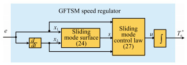 图 3 Block diagram of the designed GFTSM speed regulator.Fig. 3 Block diagram of the designed GFTSM speed regulator.
By solving differential equation (26), the time from any state $s(0)\neq 0$ to the sliding mode surface $s(t_f)$ can be derived as follows:
$ \begin{align} % eq:(28) t_f=\frac{m}{ \varphi(m-v)}\ln\frac{\varphi\left(s(0)\right)^\frac{m-v}{m}+\gamma}{ \gamma}. \end{align} $
(28) Remark 7: From (27), it can be seen that the sliding mode control law does not include switching item and thus weakens system chatter.
Remark 8: Under control law (27), one can easily see that if it converges to zero according to the terminal attractor (26), $x_1$ will accordingly converge to zero in terms of the following fast terminal attractor
$ \begin{align} % eq:(29) \dot{x}_{1}=-\alpha x_{1}-\beta x_{1}^\frac{q}{p}. \end{align} $
(29) It can be observed from (26) and (29) that the fast terminal attractors are adopted both in the reaching phase and in sliding phase. Consequently, the designed regulator (27) is a global terminal sliding mode one which guarantees the finite time control performance.
Remark 9: According to (28), $t_f$ can be set arbitrarily by adjusting parameters $m$, $v$, $\varphi$, $\gamma$.
Remark 10: The designed GFTSM speed regulator (27) is not only stable but also robust, which will be analyzed as below.
3.2.2 Stability Analysis
Construct Lyapunov function as
$ \begin{align} % eq:(30) V_2=\frac{1}{2}s^{2}. \end{align} $
(30) Differentiating (30) yields
$ \dot{V}_2=s\dot{s}=-\varphi s^2-\gamma s^\frac{m+v}{m} $
since $(m+v)$ is an even number, therefore $\dot{V}=s\dot{s}<0$. According to Lyapunov stability theory, the system (23) is stable and its movement can tend to sliding mode surface and finally reach the sliding mode.
3.2.3 Robustness Analysis
Considering parameter uncertainties and external disturbances, the system (23) is rewritten as following:
$\begin{align} % eq:(31) \begin{cases} \dot{x}_{1}=x_2\\[1mm] \dot{x}_{2}=-\dfrac{B_{\rm m}}{ J}x_2-\dfrac{1}{ J}u+d(x_1, x_2) \end{cases} \end{align} $
(31) where $d(x_1, x_2)$ can be regarded as the total disturbance including uncertainties and external disturbances. Assume $| d(x_1, x_2)|$ $\leq$ $D$, $D$ is maximum value.
As for system (31), differentiating (24) yields
$ \begin{align} % eq:(32) \dot{s}=\left(\alpha-\frac{B_{\rm m}}{ J}\right)x_2-\frac{1}{ J}u+d(x_1, x_2)+\beta\frac{{d}}{{d}t}\left(x_{1}^\frac{q}{p}\right). \end{align} $
(32) Substituting (27) into (32) yields
$ \begin{align} % eq:(33) \dot{s}& =-\varphi s-\gamma s^\frac{v}{m}+d(x_1, x_2)\notag\\[1mm] & =-\varphi s-\left(\gamma-\frac{d(x_1, x_2)} {s^\frac{v}{m}}\right)s^\frac{v}{m}. \end{align} $
(33) Let
$ \begin{align} % eq:(34) \bar{\gamma}=\gamma-\frac{d(x_1, x_2)}{s^\frac{v}{m}} \end{align} $
(34) then (33) can be rewritten as
$ \begin{align} % eq:(35) \dot{s}=-\varphi s-\bar{\gamma} s^\frac{v}{m}. \end{align} $
(35) To make (35) be a fast terminal attractor, (34) must satisfy $\bar{\gamma}>0$. Therefore, the following inequality holds true
$ \gamma-\frac{d(x_1, x_2)}{s^\frac{v}{m}}>\gamma-\frac{| d(x_1, x_2)|}{| s^\frac{v}{m}|}>\gamma-\frac{D}{ | s^\frac{v}{m}|}>0 $
then we can deduce
$ \begin{align} % eq:(36) \gamma>\frac{D}{ | s^\frac{v}{m}|}. \end{align} $
(36) Equation (36) is equivalent to
$ \begin{align} % eq:(37) | s|>\left(\frac{D}{ \gamma }\right)^\frac{m}{v}. \end{align} $
(37) As a result, the fast terminal convergence region $\Delta$ is constrained by
$ \begin{align} % eq:(38) \Delta=\left\{x_1, x_2:| s|\leq \left(\frac{D}{ \gamma }\right)^\frac{m}{v}\right\}. \end{align} $
(38) Furthermore, we assume
$ \begin{align} % eq:(39) \gamma={D\over | s^\frac{v}{m}|}+\eta, ~~~\eta>0. \end{align} $
(39) According to (35), the time from any state $s(0)\neq 0$ to the sliding surface is deduced as follows:
$ \begin{align} % eq:(40) \bar{t}_f={m\over \varphi(m-v)}\ln{\varphi\left(s(0)\right)^\frac{m-v}{m}+\bar{\gamma}\over \bar{\gamma}}. \end{align} $
(40) Since $\bar{\gamma}>\eta$, the following inequality can be deduced
$ \ln\frac{\varphi\left(s(0)\right)^\frac{m-v}{m}+\bar{\gamma}}{ \bar{\gamma}}\leq \ln\frac{\varphi\left(s(0)\right)^\frac{m-v}{m}+\eta}{ \eta} $
and then the reaching time satisfies
$ \begin{align} % eq:(41) \bar{t}_f\leq\frac{m}{ \varphi(m-v)}\ln\frac{\varphi\left(s(0)\right)^\frac{m-v}{m}+\eta}{ \eta}. \end{align} $
(41) Through the above analysis, it can be seen that if the condition $\bar{\gamma}>0$ holds then fast terminal convergence can be guaranteed and system (31) can reach neighborhood $\Delta$ of the sliding mode surface $s(\bar{t}_f)=0$ in finite time $\bar{t}_f$.
3.3 Model Predictive Torque Control
The basic idea of MPTC is to predict the future behavior of the variables over a time frame based on the model of the system. As shown in Fig. 1, MPTC includes three parts: cost function minimization, predictive model and flux and torque estimator.
3.3.1 Cost Function Minimization
For MPTC, the cost function is chosen such that both torque and flux at the end of the cycle is as close as possible to the reference value. Generally, the minimum value of cost function is defined as
$ \begin{align} % eq:(42) &\min g =\left| T_{\rm e}^{\ast}-T_{\rm e}^{k+1}\right|+k_3\left| \left| \psi_{\rm s}^{\ast}\right|-| \psi_{\rm s}^{k+1}| \right|\notag \\ &\, {\rm s.t.}\quad u_{\rm s}^{k}\in\{V_1, V_2, \ldots, V_6\} \end{align} $
(42) where $V_1$, $V_2$, $V_3$, $V_4$, $V_5$, and $V_6$ are six nonzero voltage space vectors and can be generated by three phase VSI with respect to the different switches states. A set of voltage space vectors $u_{\rm s}^{k}$ at $k$th instant is defined as
$ \begin{align} % eq:(43) u_{\rm s}^{k}=\frac{2V_{\rm dc}\left[S_{\rm a}^{k}+e^\frac{i2\pi}{3}S_{\rm b}^{k}+(e^\frac{i2\pi}{3})^{2}S_{\rm c}^{k}\right]}{3} \end{align} $
(43) where $S_{\rm a}^{k}~(x=a, b, c)$ at $k$th instant is upper power switch state of one of three legs. $S_{\rm a}^{k}=1$ or $S_{\rm a}^{k}=0$ when upper power switch of one leg is on or off. $k_3$ is the weighting factor.
In order to compensate inherent one-step delay which exists in practical digital system, the cost function (42) is revised as below:
$ \begin{align} % eq:(44) &\min g =\left| T_{\rm e}^{\ast}-T_{\rm e}^{k+2}\right|+k_3\left| \left| \psi_{\rm s}^{\ast}\right|-| \psi_{\rm s}^{k+2}| \right|\notag \\ &\, {\rm s.t.}\quad u_{\rm s}^{k}\in\{V_1, V_2, \ldots, V_6\}. \end{align} $
(44) 3.3.2 Predictive Model for Stator Currents
According to (1), the prediction of the stator current at the next sampling instant is expressed as
$ \begin{align} % eq:(45) \begin{cases} i_{\rm d}^{k+1}=i_{\rm d}^{k}+\dfrac{1}{L}\left(u_{\rm d}^{k}-R_{\rm s}i_{\rm d}^{k}+p\omega_{\rm r}^{k}Li_{\rm q}^{k}\right)T_{\rm s}\\[3mm] i_{\rm q}^{k+1}=i_{\rm q}^{k}+\dfrac{1}{ L}\left (u_{\rm q}^{k}-R_{\rm s}i_{\rm q}^{k}-p\omega_{\rm r}^{k} (Li_{\rm d}^{k}+\psi_{\rm m})\right)T_{\rm s} \end{cases} \end{align} $
(45) where $i_{\rm d}^{k}$, $i_{\rm q}^{k}$ and $R_{\rm s}$ are replaced by the corresponding estimated values coming from the observer in Fig. 2. $T_{\rm s}$ is the sampling period.
3.3.3 Torque and Flux Estimators
In $dq$-frame, the current-based flux-linkage can be expressed as following vector:
$ \begin{align} \left[% eq:(46) \begin{array}{c} \psi_{\rm d}^{k+1} \\ \psi_{\rm q}^{k+1} \\ \end{array} \right]=\left[ \begin{array}{cc} L&0 \\ 0&L \\ \end{array} \right]\left[ \begin{array}{c} i_{\rm d}^{k+1} \\ i_{\rm q}^{k+1}\\ \end{array} \right]+\left[ \begin{array}{c} \psi_{\rm m} \\ 0 \\ \end{array} \right]. \end{align} $
(46) The magnitude of stator flux linkage $\psi_{\rm s}$ is
$ \begin{align} % eq:(47) \psi_{\rm s}^{k+1}=\sqrt{(\psi_{\rm d}^{k+1})^2+(\psi_{\rm q}^{k+1})^2}. \end{align} $
(47) Electromagnetic torque developed in $dq$-frame can be estimated as following:
$ \begin{align} % eq:(48) T_{\rm e}^{k+1}=\frac{3}{ 2}{ p}\psi_{\rm m}i_{\rm q}^{k+1}. \end{align} $
(48) Substituting (45) into (48), the torque can be calculated.
4. Simulation Result and Analysis
In order to validate the effectiveness of proposed control strategy, the designed control system as shown in Fig. 1 has been implemented in MATLAB/Simulink/Simscape platform. The parameters of PMSM drive are given in Table Ⅰ. The sampling period is 100 $\mu$s, and value $k_3$ is selected to be 200. The reference stator flux $\psi_{\rm s}^{\ast}$ is 0.175 Wb. The parameters of the adaptive observer are
$ \begin{align*} &K_{P(R_{\rm s})}=0.006, ~~~K_{I(R_{\rm s})}=8\\ &k_1=30, ~~~k_2=5000, ~~~r=1000. \end{align*} $
表 Ⅰ PARAMETERS OF PMSM DRIVETable Ⅰ PARAMETERS OF PMSM DRIVESymbol Value Symbol Value $R_{\rm s}$ $2.875\, \Omega$ $\omega_{\rm r}^{\ast}$ 1000 rpm $L_{\rm d}, L_{\rm q}$ 0.0085 H $T_{\rm n}$ 4 N$\cdot$m $\psi_{\rm m}$ 0.175 Wb $J$ $0.0008\, {\rm Kg\cdot m}^2$ $p$ 4 $B_{\rm m}$ 0.001 N$\cdot$m$\cdot$s $V_{\rm dc}$ 300 V $T_{\rm f}$ 0 The parameters of GFTSM in Fig. 3 are determined as follows:
$ \begin{align*} &\alpha=100, ~~~\beta=250, ~~~p=7, ~~~q=5\\ &\varphi=1000, ~~~\gamma=80\, 000, ~~~ m=3, ~~~v=1.\end{align*} $
4.1 The GFTSM-based MPTC PMSM Drive System Comparison Between the One With Single Phase Current Sensor and the Other With Two Phase Current Sensors
In order to verify estimation accuracy of the observer for GFTSM-based MPTC PMSM drive system with single phase current sensor, two scenarios of numerical simulation are provided and compared, which correspond to PMSM system with two phase current sensors (phase-$a$ and -$b$ sensors) and PMSM system with single phase current sensor (phase-$b$), respectively. For convenience sake, the former scenario is marked as Case 1 and the latter one as Case 2. Except the above-mentioned different number of current sensors, the two systems employ completely identical GFTSM-based MPTC strategy.
Fig. 4 shows comparison of two scenarios in terms of stator currents, stator resistance, rotor speed and torque when the reference speed $n^{\ast}$ is set to 1000 pm, the load torque is increased from 0 N$\cdot$m to 4 N$\cdot$m at 0.1 seconds and the stator resistance is changed from its nominal value 2.875 $\Omega$ to 5 $\Omega$ at 0.3 seconds.
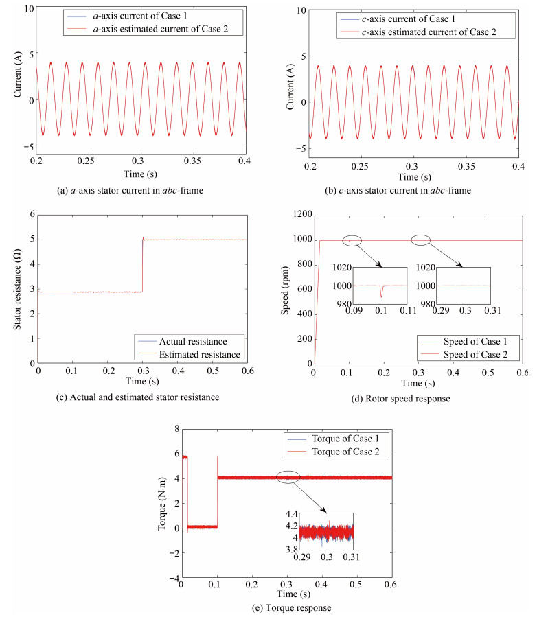 图 4 Dynamic response comparison between Case 1 and Case 2 under the variation of stator resistance.Fig. 4 Dynamic response comparison between Case 1 and Case 2 under the variation of stator resistance.
From Figs. 4(a)$-$4(c), it can be seen that, for designed adaptive observer of Case 2, its estimated $a$-axis and $c$-axis currents in $abc$-frame rapidly track corresponding ones of Case 1, and its estimated stator resistance can rapidly follow actual resistance change and converge to its actual value accurately. Figs. 4(d)$-$4(e) show that, for GFTSM-based MPTC system of Case 2, its speed and torque can be regulated in a satisfactory manner and it has almost as good performance as GFTSM-based MPTC system of Case 1.
4.2 The MPTC PMSM System Comparison Between the One Based on PI and the Other Based on GFTSM
For GFTSM-based MPTC PMSM systems, for the sake of verifying its stronger robustness, two systems are compared, which correspond to the PI-based and GFTSM-based MPTC PMSM systems, respectively. Except distinct outer-loop speed regulator (i.e., PI and GFTSM), the two systems employ completely identical MPTC and adaptive observer. In the simulation, their reference speeds $n^{\ast}$ are set to 1000 rpm, their load torques of 0 N$\cdot$m are increased to 4 N$\cdot$m at 0.1 seconds and stator resistance is at its nominal value 2.875 $\Omega$.
In the simulation, sampling values of three-phase currents are recorded over the time range from 0.1 seconds to 0.2 seconds. During this period, the fundamental frequency of three-phase currents is 66.67 Hz. Total harmonic distortion (THD) can be obtained by comparing the higher frequency components to the fundamental one.
4.2.1 The Comparison of Anti-load Variation Ability Under the Same Speed Transient Response
The parameters of PI for PI-based MPTC PMSM system are adjusted as follows:
$ K_P=0.7, ~~~K_I=0.03 $
such that PI-based MPTC system has almost the same speed transient response as GFTSM-based one.
Fig. 5 shows the dynamical responses in terms of speed, torque and stator currents. Fig. 5(a) intuitively gives the speed response comparison, which demonstrates that for GFTSM-based MPTC PMSM system, its speed can sharply adapt to the change of external load in a satisfactory manner, and its capability of accommodating the challenge of load disturbance is superior to PI-based one's. From Figs. 5(b)$-$5(d), it can be observed that for two systems with same adaptive observer, their torques, estimated $a$-axis and $c$-axis currents in $abc$-frame are almost the same.
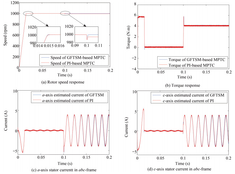 图 5 The comparison of anti-load variation ability under the same speed transient response.Fig. 5 The comparison of anti-load variation ability under the same speed transient response.
Table Ⅱ shows THD comparison of three-phase currents. From Table Ⅱ, what can be observed is that the THD of the GFTSM-based MPTC is smaller than one of the PI-based MPTC.
表 Ⅱ THD OF THREE-PHASE STATORS' CURRENT(%)Table Ⅱ THD OF THREE-PHASE STATORS' CURRENT(%)Control scheme $i_{\rm a}$ $i_{\rm b}$ $i_{\rm c}$ PI-based MPTC $2.21$ $2.32$ $2.24$ GFTSM-based MPTC $1.84$ $1.88$ $1.85$ 4.2.2 The Comparison of Dynamic Responses Under the Same Speed Anti-load Variation Ability
The parameters of PI for PI-based MPTC PMSM system are adjusted as follows:
$ K_P=3, ~~~K_I=0.1 $
such that PI-based MPTC system has almost the same anti-load variation ability as GFTSM-based one.
Figs. 6(a)$-$6(d) show the dynamical responses in terms of speed, torque and stator currents. Fig. 6(a) intuitively gives their speed response comparison, which indicates that GFTSM-based MPTC PMSM system has smaller overshoot and faster settling time than PI-based one. Meanwhile, it can be found from Fig. 6(b) that the torque response of GFTSM-based MPTC PMSM system is better than one of PI-based. From Figs. 6(c)$-$6(d), it can be observed that, their estimated $a$-axis and $c$-axis currents in $abc$-frame are almost the same.
 图 6 The comparison of dynamical response under the same speed anti-load variation ability.Fig. 6 The comparison of dynamical response under the same speed anti-load variation ability.
4.3 The MPTC PMSM System Comparison Between the One Based on SM and the Other Based on GFTSM
Here, the working condition of PMSM drive system is identical with Section 4.2.
For SM-based speed regulator, its sliding mode surface and its reaching law are selected as following:
$ s=ce+\dot{e} $
(49) $ \dot{s}=-k_4s-\varepsilon {\rm sign}(s) $
(50) 4.3.1 The Comparison of Anti-load Variation Ability Under the Same Speed Transient Response
The parameters of SM for SM-based MPTC PMSM system are adjusted as follows:
$ c=160, ~~~k_4=800, ~~~\varepsilon=3\times 10^5 $
such that SM-based MPTC system has almost the same speed transient response as GFTSM-based one.
Figs. 7(a)$-$7(d) show the dynamical responses in terms of speed, torque and stator currents. Fig. 7(a) illustrates that for GFTSM-based MPTC PMSM system, benefiting from the fast terminal sliding mode employed in both the reaching stage and the sliding stage, its recovery rate of speed response is obviously faster than SM-based one. From Figs. 7(b)$-$7(d), it can be seen that for two systems with same adaptive observer, their torques, estimated $a$-axis and $c$-axis currents in $abc$-frame are almost the same.
 图 7 The comparison of anti-load variation ability under the same speed transient response.Fig. 7 The comparison of anti-load variation ability under the same speed transient response.
Table Ⅲ shows THD comparison of three-phase currents. From Table Ⅲ, what can be observed is that the THD of the GFTSM-based MPTC is smaller than one of the SM-based MPTC.
表 Ⅲ THD OF THREE-PHASE STATORS' CURRENT(%)Table Ⅲ THD OF THREE-PHASE STATORS' CURRENT(%)Control scheme $i_{\rm a}$ $i_{\rm b}$ $i_{\rm c}$ SM-based MPTC $2.01$ $2.12$ $2.14$ GFTSM-based MPTC $1.84$ $1.88$ $1.85$ 4.3.2 The Comparison of Dynamic Response Under the Same Speed Anti-load Variation Ability
The parameters of SM for SM-based MPTC PMSM system are adjusted as follows:
$ c=140, ~~k_4=2500, ~~\varepsilon=3\times 10^7 $
such that SM-based MPTC system has almost the same anti-load variation ability as GFTSM-based one.
Figs. 8(a)$-$8(d) show the dynamical responses in terms of speed, torque and stator currents. Fig. 8(a) shows that the speed dynamic performance is better than SM-based one. And it can be found from Figs. 8(b)$-$8(d) that for SM-based MPTC PMSM system, due to a switching function sign$(\cdot)$ in (50), therefore its torque, estimated $a$-axis and $c$-axis currents have significantly heavy chatter. On the other hand, for GFTSM-based one, its sliding reaching law in (26) is a continuous and smooth function, so the system chatter can be greatly reduced.
 图 8 The comparison of dynamic response under the same anti-load variation ability.Fig. 8 The comparison of dynamic response under the same anti-load variation ability.
Summarizing above simulation experiments, we can obtain following results,
1) The proposed adaptive observer can estimate the remaining two phase currents and stator resistance rapidly and accurately.
2) Compared with PI-based and SM-based MPTC PMSM drive systems, GFTSM-based one has better dynamical response behavior and stronger robustness as well as smaller THD index of three-phase stator current.
5. Conclusions
This paper has put forward a novel GFTSM-based MPTC strategy for PMSM drive system with only one phase current sensor. Firstly, an adaptive observer is designed, which is capable of concurrent online estimation of the remaining two phase currents and time-varying stator resistance rapidly and accurately. Secondly, GFTSM speed regulator is designed and its stability and convergence as well as robustness are analytically verified based on Lyapunov stability theory. Finally, the MPTC strategy is employed to reduce the torque and flux ripples. The proposed observer can be embedded into a fault resilient PMSM drive system. In case of a phase current sensor failure, the designed observer can be used as a virtual current sensor which is robust against variation of stator resistance. And the designed GFTSM controller can enhance speed regulator's robustness against variation of system parameters and external disturbance. The resultant GFTSM-based MPTC strategy can guarantee that PMSM drive system with single phase current sensor achieves not only fast response but also high-precision control performance as well as strong robustness.
Our future research topic is that considering both parameters uncertainties and unmodeled dynamics, we will employ adaptive robust method with extended state observer to reconstruct stator currents observer.
-
表 1 不同的可诊断性对应不同故障诊断深度
Table 1 Different kinds of diagnosabilities correspond to different degrees of fault diagnosis
可诊断性分类 故障诊断深度要求 功能模块级可诊断性 确定发生故障的功能模块 部件级可诊断性 确定发生故障的部件 系统级可诊断性 确定系统是否发生故障  下载: 导出CSV
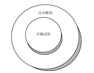
表 2 可诊断性与可测试性之间的对比分析
Table 2 The comparative analysis of diagnosability and testability
可测试性 可诊断性 本质 设计特性 研究目标 处理故障 研究方法 主要采用多信号流图方法 多信号流图, 基于数据、统计特性相似度度量等方法 度量指标 故障检测率, 故障隔离率, 故障虚警率 可检测性, 可隔离性, 可辨识性 应用范围 优化系统配置 优化系统配置, 优化诊断方案 关系 可诊断性包含可测试性
下载: 导出CSV
表 3 可诊断性与能观测性、可重构性之间的对比结果
Table 3 The comparisons of diagnosability, observability and reconfigurability
能观测性 可诊断性 可重构性 基本概念 系统状态运动可由输出完全反映的属性 系统故障能够被确定和有效地识别的程度 发生故障时, 系统克服故障恢复既定功能的能力 两者关系 能观测性分析是研究可诊断性的一种方法 处理故障的不同阶段所对应的性质
下载: 导出CSV
表 4 不同可诊断性评价方法的优越性及其局限性
Table 4 The superiority and limitation of different kinds of diagnosability evaluation methods
评价方法 优越性 局限性 基于定量模型 物理意义明确 难以获得精确模型 基于定性模型 宏观描述系统 对专业知识及经验要求较高 基于数据 不需要建立系统模型 运算量大, 难以评价未知故障
下载: 导出CSV
-
[1] Biswal M, Brahma S M, Cao H P.Supervisory protection and automated event diagnosis using PMU data.IEEE Transactions on Power Delivery, 2016, 31(4):1855-1863 doi: 10.1109/TPWRD.2016.2520958 [2] Teixeira A, Shames I, Sandberg H, Johansson K H.A secure control framework for resource-limited adversaries.Automatica, 2015, 51:135-148 doi: 10.1016/j.automatica.2014.10.067 [3] Keliris C, Polycarpou M M, Parisini T.An integrated learning and filtering approach for fault diagnosis of a class of nonlinear dynamical systems.IEEE Transactions on Neural Networks and Learning Systems, 2017, 28(4):988-1004 doi: 10.1109/TNNLS.2015.2504418 [4] Gao Z W, Ding S X, Cecati C.Real-time fault diagnosis and fault-tolerant control.IEEE Transactions on Industrial Electronics, 2015, 62(6):3752-3756 doi: 10.1109/TIE.2015.2417511 [5] Jiang B, Staroswiecki M, Cocquempot V.Fault accommodation for nonlinear dynamic systems.IEEE Transactions on Automatic Control, 2006, 51(9):1578-1583 doi: 10.1109/TAC.2006.878732 [6] Wang T Z, Qi J, Xu H, Wang Y D, Liu L, Gao D J.Fault diagnosis method based on FFT-RPCA-SVM for cascaded-multilevel inverter.ISA Transactions, 2016, 60:156-163 doi: 10.1016/j.isatra.2015.11.018 [7] Tang B P, Song T, Li F, Deng L.Fault diagnosis for a wind turbine transmission system based on manifold learning and Shannon wavelet support vector machine.Renewable Energy, 2014, 62:1-9 doi: 10.1016/j.renene.2013.06.025 [8] Yin S, Zhu X P.Intelligent particle filter and its application to fault detection of nonlinear system.IEEE Transactions on Industrial Electronics, 2015, 62(6):3852-3861 http://www.wanfangdata.com.cn/details/detail.do?_type=perio&id=JJ0234617504 [9] Sun F C, Liu H P, He K Z, Sun Z Q.Reduced-order H∞ filtering for linear systems with Markovian jump parameters.Systems and Control Letters, 2005, 54(8):739-746 doi: 10.1016/j.sysconle.2004.11.012 [10] 化永朝, 李清东, 任章, 刘成瑞.连续系统故障可诊断性评价方法综述.控制与决策, 2016, 31(12):2113-2121 http://d.old.wanfangdata.com.cn/Periodical/kzyjc201612001Hua Yong-Zhao, Li Qing-Dong, Ren Zhang, Liu ChengRui.Overview of fault diagnosability evaluation methods for continuous systems.Control and Decision, 2016, 31(12):2113-2121 http://d.old.wanfangdata.com.cn/Periodical/kzyjc201612001 [11] 刘文静, 刘成瑞, 王南华.故障可诊断性评价与设计研究进展.航天控制, 2011, 29(6):72-78, 87 http://d.old.wanfangdata.com.cn/Periodical/htkz201106015Liu Wen-Jing, Liu Cheng-Rui, Wang Nan-Hua.Overview of fault diagnosability evaluation and design.Aerospace Control, 2011, 29(6):72-78, 87 http://d.old.wanfangdata.com.cn/Periodical/htkz201106015 [12] IEEE Trial-Use Standard for Testability and Diagnosability Characteristics and Metrics, IEEE Standard 1522, 2004. [13] Wang D W, Yu M, Low C B, Arogeti S.Modelbased Health Monitoring of Hybrid Systems.New York:Springer, 2013.2-16 [14] Gertler J.Fault Detection and Diagnosis in Engineering Systems.New York:Marcel Dekker, 1998.1-22 [15] Ding S X.Model-based Fault Diagnosis Techniques:Design Schemes, Algorithms and Tools.Berlin Heidelberg:Springer-Verlag, 2008.51-68 [16] Chi G Y, Wang D W, Zhu S Q.An integrated approach for sensor placement in linear dynamic systems.Journal of the Franklin Institute, 2015, 352(3):1056-1079 doi: 10.1016/j.jfranklin.2014.11.013 [17] Eriksson D, Frisk E, Krysander M.A method for quantitative fault diagnosability analysis of stochastic linear descriptor models.Automatica, 2013, 49(6):1591-1600 doi: 10.1016/j.automatica.2013.02.045 [18] Scott J K, Findeisen R, Braatz R D, Raimondo D M.Design of active inputs for set-based fault diagnosis.In: Proceedings of the 2013 American Control Conference.Washington, DC, USA: IEEE, 2013.3561-3566 [19] Düştegör D, Frisk E, Cocquempot V, Krysander M, Staroswiecki M.Structural analysis of fault isolability in the DAMADICS benchmark.Control Engineering Practice, 2006, 14(6):597-608 doi: 10.1016/j.conengprac.2005.04.008 [20] Krysander M, Frisk E.Sensor placement for fault diagnosis.IEEE Transactions on Systems, Man, and Cybernetics, Part A:Systems and Humans, 2008, 38(6):1398-1410 doi: 10.1109/TSMCA.2008.2003968 [21] Leal R, Aguilar J, Travé-Massuyés L, Camargo E, Ríos A.An approach for diagnosability analysis and sensor placement for continuous processes based on evolutionary algorithms and analytical redundancy.Applied Mathematical Sciences, 2015, 9(43):2125-2146 http://www.academia.edu/20214521/An_Approach_for_Diagnosability_Analysis_and_Sensor_Placement_for_Continuous_Processes_Based_on_Evolutionary_Algorithms_and_Analytical_Redundancy [22] Sun F C, Li L, Li H X, Liu H P.Neuro-fuzzy dynamicinversion-based adaptive control for robotic manipulators-discrete time case.IEEE Transactions on Industrial Electronics, 2007, 54(3):1342-1351 doi: 10.1109/TIE.2007.893056 [23] Sun F C, Li H X, Lei L.Robot discrete adaptive control based on dynamic inversion using dynamical neural networks.Automatica, 2002, 38(11):1977-1983 doi: 10.1016/S0005-1098(02)00116-4 [24] Zheng W H, Jia Y M.Leader-follower formation control of mobile robots with sliding mode.Journal of Robotics, Networking and Artificial Life, 2017, 4(1):10-13 doi: 10.2991/jrnal.2017.4.1.3 [25] Gertler J J.Survey of model-based failure detection and isolation in complex plants.IEEE Control Systems Magazine, 1988, 8(6):3-11 doi: 10.1109/37.9163 [26] Kouadri A, Bensmail A, Kheldoun A, Refoufi L.An adaptive threshold estimation scheme for abrupt changes detection algorithm in a cement rotary kiln.Journal of Computational and Applied Mathematics, 2014, 259:835-842 doi: 10.1016/j.cam.2013.07.039 [27] 符方舟, 王大轶, 李文博.基于卡尔曼滤波器组的多重故障诊断方法研究.控制理论与应用, 2017, 34(5):586-593 http://d.old.wanfangdata.com.cn/Periodical/kzllyyy201705004Fu Fang-Zhou, Wang Da-Yi, Li Wen-Bo.Multiple fault detection and isolation based on Kalman filters.Control Theory and Applications, 2017, 34(5):586-593 http://d.old.wanfangdata.com.cn/Periodical/kzllyyy201705004 [28] Niu G, Zhao Y J, Tran V T.Fault detection and isolation based on bond graph modeling and empirical residual evaluation.Proceedings of the Institution of Mechanical Engineers, Part C:Journal of Mechanical Engineering Science, 2015, 229(3):417-428 doi: 10.1177/0954406214536381 [29] Chilin D, Liu J F, Chen X Z, Christofides P D.Fault detection and isolation and fault tolerant control of a catalytic alkylation of benzene process.Chemical Engineering Science, 2012, 78:155-166 doi: 10.1016/j.ces.2012.05.015 [30] 符方舟, 王大轶, 李文博.基于分层随机梯度辨识算法的传感器故障检测方法.空间控制技术与应用, 2016, 42(4):12-17 doi: 10.3969/j.issn.1674-1579.2016.04.003Fu Fang-Zhou, Wang Da-Yi, Li Wen-Bo.Sensor fault detection based on hierarchical stochastic gradient identification algorithm.Aerospace Control and Application, 2016, 42(4):12-17 doi: 10.3969/j.issn.1674-1579.2016.04.003 [31] 国家标准.GJB 451A-2005可靠性维修性保障性术语, 2005.National Standard.GJB 451A-2005 Reliability, Maintainability and Supportability Terms, 2005. [32] Frank P M.Fault diagnosis in dynamic systems using analytical and knowledge-based redundancy:a survey and some new results.Automatica, 1990, 26(3):459-474 doi: 10.1016/0005-1098(90)90018-D [33] Venkatasubramanian V, Rengaswamy R, Yin K, Kavuri S N.A review of process fault detection and diagnosis, Part Ⅰ:quantitative model-based methods.Computers and Chemical Engineering, 2003, 27(3):293-311 doi: 10.1016/S0098-1354(02)00160-6 [34] Venkatasubramanian V, Rengaswamy R, Kavuri S N.A review of process fault detection and diagnosis, Part Ⅱ:qualitative models and search strategies.Computers and Chemical Engineering, 2003, 27(3):313-326 doi: 10.1016/S0098-1354(02)00161-8 [35] Venkatasubramanian V, Rengaswamy R, Kavuri S N, Yin K.A review of process fault detection and diagnosis, Part Ⅲ:process history based methods.Computers and Chemical Engineering, 2003, 27(3):327-346 doi: 10.1016/S0098-1354(02)00162-X [36] 李娟, 周东华, 司小胜, 陈茂银, 徐春红.微小故障诊断方法综述.控制理论与应用, 2012, 29(12):1517-1529 http://d.old.wanfangdata.com.cn/Periodical/kzllyyy201212001Li Juan, Zhou Dong-Hua, Si Xiao-Sheng, Chen Mao-Yin, Xu Chun-Hong.Review of incipient fault diagnosis methods.Control Theory and Applications, 2012, 29(12):1517-1529 http://d.old.wanfangdata.com.cn/Periodical/kzllyyy201212001 [37] 周东华, 史建涛, 何潇.动态系统间歇故障诊断技术综述.自动化学报, 2014, 40(2):161-171 http://www.aas.net.cn/CN/abstract/abstract18279.shtmlZhou Dong-Hua, Shi Jian-Tao, He Xiao.Review of intermittent fault diagnosis techniques for dynamic systems.Acta Automatica Sinica, 2014, 40(2):161-171 http://www.aas.net.cn/CN/abstract/abstract18279.shtml [38] Zhang B, Jia Y M, Matsuno F, Endo T.Task-space synchronization of networked mechanical systems with uncertain parameters and communication delays.IEEE Transactions on Cybernetics, 2017, 47(8):2288-2298 doi: 10.1109/TCYB.2016.2597446 [39] Apkarian P, Gahinet P.A convex characterization of gainscheduled H∞ controllers.IEEE Transactions on Automatic Control, 1995, 40(5):853-864 doi: 10.1109/9.384219 [40] Park S, Park Y, Park Y S.Degree of fault isolability and active fault diagnosis for redundantly actuated vehicle system.International Journal of Automotive Technology, 2016, 17(6):1045-1053 doi: 10.1007/s12239-016-0102-1 [41] Du Y C, Duever T A, Budman H.Fault detection and diagnosis with parametric uncertainty using generalized polynomial chaos.Computers and Chemical Engineering, 2015, 76:63-75 doi: 10.1016/j.compchemeng.2015.02.009 [42] Hou L Q, Bergmann N W.Novel industrial wireless sensor networks for machine condition monitoring and fault diagnosis.IEEE Transactions on Instrumentation and Measurement, 2012, 61(10):2787-2798 doi: 10.1109/TIM.2012.2200817 [43] Liu W J, Teng B Y.Application of weighted evidence theory in the space-earth fault diagnosis result fusion of spacecraft.In: Proceedings of the 12th World Congress on Intelligent Control and Automation.Guilin, China: IEEE, 2016.1742-1748 [44] Kelkar S, Kamal R.Adaptive fault diagnosis algorithm for controller area network.IEEE Transactions on Industrial Electronics, 2014, 61(10):5527-5537 doi: 10.1109/TIE.2013.2297296 [45] 刘文静, 王南华.面向资源约束航天器控制系统的故障检测研究.宇航学报, 2011, 32(7):1527-1533 doi: 10.3873/j.issn.1000-1328.2011.07.014Liu Wen-Jing, Wang Nan-Hua.FD for spacecraft control system with resource constraint.Journal of Astronautics, 2011, 32(7):1527-1533 doi: 10.3873/j.issn.1000-1328.2011.07.014 [46] Jia Y M.General solution to diagonal model matching control of multiple-output-delay systems and its applications in adaptive scheme.Progress in Natural Science, 2009, 19(1):79-90 doi: 10.1016/j.pnsc.2008.05.019 [47] Yang F W, Li Y M.Set-membership filtering for systems with sensor saturation.Automatica, 2009, 45(8):1896-1902 doi: 10.1016/j.automatica.2009.04.011 [48] Wang H, Huang Z J, Daley S.On the use of adaptive updating rules for actuator and sensor fault diagnosis.Automatica, 1997, 33(2):217-225 doi: 10.1016/S0005-1098(96)00155-0 [49] Ding S X, Zhong M Y, Tang B Y, Zhang P.An LMI approach to the design of fault detection filter for time-delay LTI systems with unknown inputs.In: Proceedings of the 2001 American Control Conference.Arlington, VA, USA: IEEE, 2001.2137-2142 [50] Shen Q K, Jiang B, Shi P.Active fault-tolerant control against actuator fault and performance analysis of the effect of time delay due to fault diagnosis.International Journal of Control Automation and Systems, 2017, 15(2):537-546 doi: 10.1007/s12555-015-0307-5 [51] Russell E L, Chiang L H, Braatz R D.Fault detection in industrial processes using canonical variate analysis and dynamic principal component analysis.Chemometrics and Intelligent Laboratory Systems, 2000, 51(1):81-93 doi: 10.1016/S0169-7439(00)00058-7 [52] Han L, Li C W, Guo S L, Su X W.Feature extraction method of bearing AE signal based on improved FASTICA and wavelet packet energy.Mechanical Systems and Signal Processing, 2015, 62-63:91-99 doi: 10.1016/j.ymssp.2015.03.009 [53] Sun J W, Xi L F, Pan E S, Du S C, Xia T B.Design for diagnosability of multistation manufacturing systems based on sensor allocation optimization.Computers in Industry, 2009, 60(7):501-509 doi: 10.1016/j.compind.2009.02.001 [54] Wang X Q, Zhao Y, Wang D, Zhu H J, Zhang Q.Improved multi-objective ant colony optimization algorithm and its application in complex reasoning.Chinese Journal of Mechanical Engineering, 2013, 26(5):1031-1040 doi: 10.3901/CJME.2013.05.1031 [55] Lee J M, Qin S J, Lee I B.Fault detection and diagnosis based on modified independent component analysis.AIChE Journal, 2006, 52(10):3501-3514 doi: 10.1002/(ISSN)1547-5905 [56] Ye H, Wang G, Ding S X.A new parity space approach for fault detection based on stationary wavelet transform.IEEE Transactions on Automatic Control, 2004, 49(2):281-287 doi: 10.1109/TAC.2003.822856 [57] Kaufman M, Sheppard J.P1522: a formal standard for testability and diagnosability measures.In: Proceedings of the 1999 IEEE Systems Readiness Technology Conference.San Antonio, Texas, USA: IEEE, 1999.411-418 [58] Provan G.System diagnosability analysis using modelbased diagnosis tools.In: Proceedings of the 2001 Aerospace/Def-ense Sensing, Simulation, and Controls.Orlando, FL, USA: SPIE, 2001.93-101 [59] Pattipati K R, Raghavan V, Shakeri M, Deb S, Shrestha R.TEAMS: testability engineering and maintenance system.In: Proceedings of the 1994 American Control Conference.Baltimore, Maryland, USA: IEEE, 1994.1989-1995 [60] Wey C L.Design of testability for analogue fault diagnosis.International Journal of Circuit Theory and Applications, 1987, 15(2):123-142 doi: 10.1002/(ISSN)1097-007X [61] Simpson W R, Sheppard J W.System Test and Diagnosis.US:Springer, 1994.139-190 http://d.old.wanfangdata.com.cn/Periodical/dwjs201201042 [62] Li K S M, Chang Y W, Lee C L, Su C, Chen J E.Multilevel full-chip routing with testability and yield enhancement.IEEE Transactions on Computer-Aided Design of Integrated Circuits and Systems, 2007, 26(9):1625-1636 doi: 10.1109/TCAD.2007.895587 [63] Ungar L Y.Economic evaluation of testability and diagnosability for commercial off the shelf equipment.In: Proceedings of the 2010 AUTOTESTCON.Orlando, USA: IEEE, 2010.1-5 [64] Le Traon Y, Ouabdesselam F, Robach C, Baudry B.From diagnosis to diagnosability:axiomatization, measurement and application.Journal of Systems and Software, 2003, 65(1):31-50 doi: 10.1016/S0164-1212(02)00026-2 [65] 国家标准.GJB 3385-98测试与诊断术语, 1998.National Standard.GJB 3385-98 Terms for Testing and Diagnostics, 1998. [66] Sheppard J W, Kaufman M.Formal specification of testability metrics in IEEE P1522.In: Proceedings of the 2001 IEEE Systems Readiness Technology Conference, AUTOTESTCON.Valley Forge, PA, USA: IEEE, 2001.71-82 [67] Magni J F, Mouyon P.On residual generation by observer and parity space approaches.IEEE Transactions on Automatic Control, 1994, 39(2):441-447 doi: 10.1109/9.272354 [68] Diop S, Martínez-Guerra R.On an algebraic and differential approach of nonlinear systems diagnosis.In: Proceedings of the 40th IEEE Conference on Decision and Control.Orlando, Florida, USA: IEEE, 2001.585-589 [69] Huber J, Kopecek H, Hofbaur M.Sensor selection for fault parameter identification applied to an internal combustion engine.In: Proceedings of the 2014 IEEE Conference on Control Applications.Juan Les Antibes, France: IEEE, 2014.89-96 [70] Wu N E, Zhou K M, Salomon G.Control reconfigurability of linear time-invariant systems.Automatica, 2000, 36(11):1767-1771 doi: 10.1016/S0005-1098(00)00080-7 [71] 王大轶, 屠园园, 刘成瑞, 何英姿, 李文博.航天器控制系统可重构性的内涵与研究综述.自动化学报, 2017, 43(10):1687-1702 http://www.aas.net.cn/CN/abstract/abstract19147.shtmlWang Da-Yi, Tu Yuan-Yuan, Liu Cheng-Rui, He Ying-Zi, Li Wen-Bo.Connotation and research of reconfigurability for spacecraft control systems:a review.Acta Automatica Sinica, 2017, 43(10):1687-1702 http://www.aas.net.cn/CN/abstract/abstract19147.shtml [72] Svärd C, Nyberg M, Frisk E.Realizability constrained selection of residual generators for fault diagnosis with an automotive engine application.IEEE Transactions on Systems, Man, and Cybernetics:Systems, 2013, 43(6):1354-1369 doi: 10.1109/TSMC.2013.2258906 [73] Cocquempot V, Izadi-Zamanabadi R, Staroswiecki M, Blanke M.Residual generation for the ship benchmark using structural approach.In: Proceedings of the 1998 UKACC International Conference on Control.Swansea, UK: IET, 1998.1480-1485 [74] Izadi-Zamanabadi R.Structural analysis approach to fault diagnosis with application to fixed-wing aircraft motion.In: Proceedings of the 2002 American Control Conference.Anchorage, USA: IEEE, 2002.3949-3954 [75] Bozzano M, Cimatti A, Katoen J P, Nguyen V Y, Noll T, Roveri M.The COMPASS approach: correctness, modelling and performability of aerospace systems.In: Proceedings of the 28th International Conference on Computer Safety, Reliability, and Security.Heidelberg, Berlin, Germany: Springer-Verlag, 2009.173-186 [76] Roychoudhury I, Biswas G, Koutsoukos X.Designing distributed diagnosers for complex continuous systems.IEEE Transactions on Automation Science and Engineering, 2009, 6(2):277-290 doi: 10.1109/TASE.2008.2009094 [77] Svärd C, Nyberg M.Automated design of an FDI system for the wind turbine benchmark.Journal of Control Science and Engineering, 2012, 2012: Article ID 989873 [78] Eriksson D, Krysander M, Frisk E.Quantitative fault diagnosability performance of linear dynamic descriptor models.In: Proceedings of the 22nd International Workshop on Principles of Diagnosis.Murnau, Germany, 2011.1-8 [79] Hao J J, Kinnaert M.Sensor fault detection and isolation over wireless sensor network based on hardware redundancy.Journal of Physics:Conference Series, 2017, 783(1):012006 http://difusion.ulb.ac.be/vufind/Record/ULB-DIPOT:oai:dipot.ulb.ac.be:2013/247702/Details [80] Chen J L, Sun H L, Wang S, He Z J.Quantitative index and abnormal alarm strategy using sensor-dependent vibration data for blade crack identification in centrifugal booster fans.Sensors, 2016, 16(5):632 doi: 10.3390/s16050632 [81] Sharifi R, Langari R.Sensor fault diagnosis with a probabilistic decision process.Mechanical Systems and Signal Processing, 2013, 34(1-2):146-155 doi: 10.1016/j.ymssp.2012.07.014 [82] Varga A.Solving Fault Diagnosis Problems.New York:Springer, 2017.9-25 [83] Patton R J, Chen J.Observer-based fault detection and isolation:robustness and applications.Control Engineering Practice, 1997, 5(5):671-682 doi: 10.1016/S0967-0661(97)00049-X [84] Del Gobbo D, Napolitano M R.Issues in fault detectability for dynamic systems.In: Proceedings of the 2000 American Control Conference.Chicago, Illinois, USA: IEEE, 2000.3203-3207 [85] Varga A.Design of fault detection filters for periodic systems.In: Proceedings of the 40th IEEE Conference on Decision and Control.Nassau, Bahamas: IEEE, 2004.4800-4805 [86] Kóscielny J M, Syfert M, Rostek K, Sztyber A.Fault isolability with different forms of the faults-symptoms relation.International Journal of Applied Mathematics and Computer Science, 2016, 26(4):815-826 doi: 10.1515/amcs-2016-0058 [87] Nyberg M.Criterions for detectability and strong detectability of faults in linear systems.International Journal of Control, 2002, 75(7):490-501 doi: 10.1080/00207170110121303 [88] Heintz F, Krysander M, Roll J, Frisk E.FlexDx: a reconfigurable diagnosis framework.In: Proceedings of the 19th International Workshop on Principles of Diagnosis DX.Blue Mountains, Australia, 2008.79-86 [89] Nyberg M, Frisk E.Residual generation for fault diagnosis of systems described by linear differential-algebraic equations.IEEE Transactions on Automatic Control, 2006, 51(12):1995-2000 doi: 10.1109/TAC.2006.884960 [90] Liu B, Si J.Fault isolation filter design for linear timeinvariant systems.IEEE Transactions on Automatic Control, 1997, 42(5):704-707 doi: 10.1109/9.580881 [91] Ding Y, Shi J J, Ceglarek D.Diagnosability analysis of multi-station manufacturing processes.Journal of Dynamic Systems, Measurement, and Control, 2001, 124(1):1-13 http://www.wanfangdata.com.cn/details/detail.do?_type=perio&id=CC027191526 [92] 李文博, 王大轶, 刘成瑞.有干扰的控制系统故障可诊断性量化评估.控制理论与应用, 2015, 32(6):744-752 http://d.old.wanfangdata.com.cn/Periodical/kzllyyy201506004Li Wen-Bo, Wang Da-Yi, Liu Cheng-Rui.Quantitative fault diagnosis ability evaluation for control systems with disturbances.Control Theory and Applications, 2015, 32(6):744-752 http://d.old.wanfangdata.com.cn/Periodical/kzllyyy201506004 [93] 符方舟, 王大轶, 李文博.复杂动态系统的实际非完全失效故障的可诊断性评估.自动化学报, 2017, 43(11):1941-1949 http://www.aas.net.cn/CN/abstract/abstract19169.shtmlFu Fang-Zhou, Wang Da-Yi, Li Wen-Bo.Quantitative evaluation of actual LOE fault diagnosability for dynamic systems.Acta Automatica Sinica, 2017, 43(11):1941-1949 http://www.aas.net.cn/CN/abstract/abstract19169.shtml [94] 李文博, 王大轶, 刘成瑞.动态系统实际故障可诊断性的量化评价研究.自动化学报, 2015, 41(3):497-507 http://www.aas.net.cn/CN/abstract/abstract18628.shtmlLi Wen-Bo, Wang Da-Yi, Liu Cheng-Rui.Quantitative evaluation of actual fault diagnosability for dynamic systems.Acta Automatica Sinica, 2015, 41(3):497-507 http://www.aas.net.cn/CN/abstract/abstract18628.shtml [95] 黄琳, 耿志勇, 王金枝, 段志生, 杨莹.控制与本质非线性问题.自动化学报, 2007, 33(10):1009-1013 http://www.aas.net.cn/CN/abstract/abstract15810.shtmlHuang Lin, Geng Zhi-Yong, Wang Jin-Zhi, Duan ZhiSheng, Yang Ying.Problems in control and intrinsic nonlinearities.Acta Automatica Sinica, 2007, 33(10):1009-1013 http://www.aas.net.cn/CN/abstract/abstract15810.shtml [96] Frisk E, Åslund J.Lowering orders of derivatives in nonlinear residual generation using realization theory.Automatica, 2005, 41(10):1799-1807 doi: 10.1016/j.automatica.2005.04.022 [97] Zhang X D, Parisini T, Polycarpou M M.Sensor bias fault isolation in a class of nonlinear systems.IEEE Transactions on Automatic Control, 2005, 50(3):370-376 doi: 10.1109/TAC.2005.843875 [98] Zhang X D.Sensor bias fault detection and isolation in a class of nonlinear uncertain systems using adaptive estimation.IEEE Transactions on Automatic Control, 2011, 56(5):1220-1226 doi: 10.1109/TAC.2011.2112471 [99] Ferrari R M G, Parisini T, Polycarpou M M.Distributed fault detection and isolation of large-scale discrete-time nonlinear systems:an adaptive approximation approach.IEEE Transactions on Automatic Control, 2012, 57(2):275-290 doi: 10.1109/TAC.2011.2164734 [100] Peng X F, Lin L X, Zhong X Y, Liu C R.Methods for fault diagnosability analysis of a class of affine nonlinear systems.Mathematical Problems in Engineering, 2015, 2015: Article ID 409184 [101] Xing Z R, Xia Y Q.Evaluation and design of actuator fault diagnosability for nonlinear affine uncertain systems with unknown indeterminate inputs.International Journal of Adaptive Control and Signal Processing, 2017, 31(1):122-137 doi: 10.1002/acs.v31.1 [102] 李文博, 王大轶, 刘成瑞.一类非线性系统的故障可诊断性量化评价方法.宇航学报, 2015, 36(4):455-462 doi: 10.3873/j.issn.1000-1328.2015.04.012Li Wen-Bo, Wang Da-Yi, Liu Cheng-Rui.An approach to fault diagnosability quantitative evaluation for a class of nonlinear systems.Journal of Astronautics, 2015, 36(4):455-462 doi: 10.3873/j.issn.1000-1328.2015.04.012 [103] 蒋栋年, 李炜, 王君.非线性系统故障可诊断性量化评价及诊断方法.华中科技大学学报:自然科学版, 2016, 44(12):102-108 http://d.old.wanfangdata.com.cn/Periodical/hzlgdxxb201612018Jiang Dong-Nian, Li Wei, Wang Jun.Fault diagnosability quantitative evaluation and method of fault diagnosis for nonlinear system.Journal of Huazhong University of Science and Technology:Natural Science Edition, 2016, 44(12):102-108 http://d.old.wanfangdata.com.cn/Periodical/hzlgdxxb201612018 [104] Cabasino M P, Giua A, Seatzu C.Diagnosability of discrete-event systems using labeled Petri nets.IEEE Transactions on Automation Science and Engineering, 2014, 11(1):144-153 doi: 10.1109/TASE.2013.2289360 [105] Haar S, Benveniste A, Fabre E, Jard C.Partial order diagnosability of discrete event systems using petri net unfoldings.In: Proceedings of the 42nd IEEE Conference on Decision and Control.Maui, HI, USA: IEEE, 2003.3748-3753 [106] Kościelny J M, Bartys M, Rzepiejewski P, Sáda Costa J.Actuator fault distinguishability study for the DAMADICS benchmark problem.Control Engineering Practice, 2006, 14(6):645-652 doi: 10.1016/j.conengprac.2005.06.014 [107] Liu J, Hua Y Z, Li Q D, Ren Z.Fault diagnosability qualitative analysis of spacecraft based on temporal fault signature matrix.In: Proceedings of the 2016 IEEE Chinese Guidance, Navigation and Control Conference.Nanjing, China: IEEE, 2017.1496-1500 [108] Mekki T, Triki S, Kamoun A.A qualitative approach to single fault isolation in switching systems.In: Proceedings of the 14th International Conference on Sciences and Techniques of Automatic Control and Computer Engineering.Sousse, Tunisia: IEEE, 2013.220-224 [109] Chittaro L, Ranon R.Hierarchical model-based diagnosis based on structural abstraction.Artificial Intelligence, 2004, 155(1-2):147-182 doi: 10.1016/j.artint.2003.06.003 [110] Genesereth M R.The use of design descriptions in automated diagnosis.Artificial Intelligence, 1984, 24(1-3):411-436 doi: 10.1016/0004-3702(84)90043-2 [111] Pucel X, Mayer W, Stumptner M.Diagnosability analysis without fault models.In: Proceedings of the 20th International Workshop on Principles of Diagnosis.Stockholm, Sweden, 2009.67-74 [112] 李晗, 萧德云.基于数据驱动的故障诊断方法综述.控制与决策, 2011, 26(1):1-9 http://d.old.wanfangdata.com.cn/Periodical/zdhxb201609001Li Han, Xiao De-Yun.Survey on data driven fault diagnosis methods.Control and Decision, 2011, 26(1):1-9 http://d.old.wanfangdata.com.cn/Periodical/zdhxb201609001 [113] Dunia R, Joe Qin S.Subspace approach to multidimensional fault identification and reconstruction.AIChE Journal, 1998, 44(8):1813-1831 doi: 10.1002/(ISSN)1547-5905 [114] Yue H H, Qin S J.Reconstruction-based fault identification using a combined index.Industrial and Engineering Chemistry Research, 2001, 40(20):4403-4414 doi: 10.1021/ie000141+ [115] Charbonnier S, Bouchair N, Gayet P.Fault template extraction to assist operators during industrial alarm floods.Engineering Applications of Artificial Intelligence, 2016, 50:32-44 doi: 10.1016/j.engappai.2015.12.007 [116] Hua Y Z, Li Q D, Ren Z, Liu C R.A data driven method for quantitative fault diagnosability evaluation.In: Proceedings of the 2016 Chinese Control and Decision Conference.Yinchuan, China: IEEE, 2016.1890-1894 [117] Ji H Q, He X, Shang J, Zhou D H.Incipient sensor fault diagnosis using moving window reconstruction-based contribution.Industrial and Engineering Chemistry Research, 2016, 55(10):2746-2759 doi: 10.1021/acs.iecr.5b03944 [118] Basseville M, Benveniste A, Moustakides G V, Rougee A.Optimal sensor location for detecting changes in dynamical behavior.IEEE Transactions on Automatic Control, 1987, 32(12):1067-1075 doi: 10.1109/TAC.1987.1104501 [119] Daigle M, Roychoudhury I, Bregon A.Diagnosabilitybased sensor placement through structural model decomposition.In: Proceedings of the 2nd European Conference of the Prognostics and Health Management Society.Nantes, France, 2014.33-46 [120] Travé-Massuyés L, Escobet T, Milne R.Model-based diagnosability and sensor placement application to a frame 6 gas turbine subsystem.In: Proceedings of the 17th International Joint Conference on Artificial Intelligence.Seattle, WA, USA: Morgan Kaufmann Publishers Inc., 2001.551-556 [121] Travé-Massuyés L, Escobet T, Olive X.Diagnosability analysis based on component-supported analytical redundancy relations.IEEE Transactions on Systems, Man, and Cybernetics, Part A:Systems and Humans, 2006, 36(6):1146-1160 doi: 10.1109/TSMCA.2006.878984 [122] Debouk R, Lafortune S, Teneketzis D.On an optimization problem in sensor selection.Discrete Event Dynamic Systems, 2002, 12(4):417-445 doi: 10.1023/A:1019770124060 [123] Frisk E, Krysander M, Åslund J.Sensor placement for fault isolation in linear differential-algebraic systems.Automatica, 2009, 45(2):364-371 doi: 10.1016/j.automatica.2008.08.013 [124] Eriksson D, Krysander M, Frisk E.Using quantitative diagnosability analysis for optimal sensor placement.IFAC Proceedings Volumes, 2012, 45(20):940-945 doi: 10.3182/20120829-3-MX-2028.00196 [125] Jung D, Eriksson L, Frisk E, Krysander M.Development of misfire detection algorithm using quantitative FDI performance analysis.Control Engineering Practice, 2015, 34:49-60 doi: 10.1016/j.conengprac.2014.10.001 [126] Nguyen D T, Duong Q B, Zamai E, Shahzad M K.Fault diagnosis for the complex manufacturing system.Proceedings of the Institution of Mechanical Engineers, Part O:Journal of Risk and Reliability, 2016, 230(2):178-194 doi: 10.1177/1748006X15623089 [127] Cui Y Q, Shi J Y, Wang Z L.System-level operational diagnosability analysis in quasi real-time fault diagnosis:the probabilistic approach.Journal of Process Control, 2014, 24(9):1444-1453 doi: 10.1016/j.jprocont.2014.06.014 [128] Kinnaert M, Hao J J.Distributed sensor fault detection and isolation over network.IFAC Proceedings Volumes, 2014, 47(3):11458-11463 doi: 10.3182/20140824-6-ZA-1003.00674 [129] Ding S X.Application of factorization and gap metric techniques to fault detection and isolation, Part Ⅰ:a factorization technique based FDI framework.IFAC-PapersOnLine, 2015, 48(21):113-118 doi: 10.1016/j.ifacol.2015.09.513 [130] Ding S X.Application of factorization and gap metric techniques to fault detection and isolation, Part Ⅱ:gap metric technique aided FDI performance analysis.IFACPapersOnLine, 2015, 48(21):119-124 https://www.sciencedirect.com/science/article/pii/S2405896315016432 [131] Eriksson D, Sundstrom C.Sequential residual generator selection for fault detection.In: Proceedings of the 2014 European Control Conference.Strasbourg, France: IEEE, 2014.932-937 [132] Bregon A, Daigle M, Roychoudhury I.An integrated framework for distributed diagnosis of process and sensor faults.In: Proceedings of the 2015 IEEE Aerospace Conference.Big Sky, MT, USA: IEEE, 2015.1-11 [133] Daigle M J, Bregon A, Koutsoukos X, Biswas G, Pulido B.A qualitative event-based approach to multiple fault diagnosis in continuous systems using structural model decomposition.Engineering Applications of Artificial Intelligence, 2016, 53:190-206 doi: 10.1016/j.engappai.2016.04.002 [134] Daigle M, Bregon A, Biswas G, Koutsoukos X, Pulido B.Improving multiple fault diagnosability using possible conflicts.IFAC Proceedings Volumes, 2012, 45(20):144-149 doi: 10.3182/20120829-3-MX-2028.00132 [135] Khorasgani H, Jung D, Biswas G.Structural approach for distributed fault detection and isolation.IFACPapersOnLine, 2015, 48(21):72-77 http://www.wanfangdata.com.cn/details/detail.do?_type=perio&id=JJ0232657451 [136] Basseville M.On fault detectability and isolability.European Journal of Control, 2001, 7(6):625-637 doi: 10.3166/ejc.7.625-637 [137] Jiang B, Chowdhury F N.Fault estimation and accommodation for linear MIMO discrete-time systems.IEEE Transactions on Control Systems Technology, 2005, 13(3):493-499 doi: 10.1109/TCST.2004.839569 [138] Joshi S M, González O R, Upchurch J M.Identifiability of additive actuator and sensor faults by state augmentation.Journal of Guidance, Control, and Dynamics, 2014, 37(3):941-946 doi: 10.2514/1.62523 [139] Upchurch J M, González O R, Joshi S M.Identifiability of Additive, Time-Varying Actuator and Sensor Faults by State Augmentation, Technical Report NASA/TM-2014-218669, L-20505, NF1676L-20305, NASA Langley Research Center, Hampton, VA, USA, 2014. [140] Ding Y, Kim P, Ceglarek D, Jin J.Optimal sensor distribution for variation diagnosis in multistation assembly processes.IEEE Transactions on Robotics and Automation, 2003, 19(4):543-556 doi: 10.1109/TRA.2003.814516 [141] Wani M F, Gandhi O P.Diagnosability evaluation of systems using bipartite graph and matrix approach.AI EDAM-Artificial Intelligence for Engineering Design Analysis and Manufacturing, 2000, 14(3):193-206 doi: 10.1017/S0890060400143021 [142] Liu Z T, Ahmed Q, Zhang J Y, Rizzoni G, He H W.Structural analysis based sensors fault detection and isolation of cylindrical lithium-ion batteries in automotive applications.Control Engineering Practice, 2016, 52:46-58 doi: 10.1016/j.conengprac.2016.03.015 [143] de Kleer J, Williams B C.Diagnosing multiple faults.Artificial Intelligence, 1987, 32(1):97-130 doi: 10.1016/0004-3702(87)90063-4 [144] Feldman A, van Gemund A.A two-step hierarchical algorithm for model-based diagnosis.In: Proceedings of the 2006 Actional Conference on Artificial Intelligence.Boston, USA: AAAI Press, 2006.827-833 [145] De Kleer J.Hitting set algorithms for model-based diagnosis.In: Proceedings of the 22nd International Workshop on Principles of Diagnosis.Murnau, Germany, 2011.1-6 [146] Console L, Picardi C, Ribaudo M.Diagnosis and diagnosability analysis using process algebras.In: Proceedings of the 14th European Conference on Artificial Intelligence.Berlin, Germany, 2000.131-135 [147] Dressler O, Struss P.A toolbox integrating model-based diagnosability analysis and automated generation of diagnostics.In: Proceedings of the 14th International Workshop on Principles of Diagnosis.USA, 2003.99-104 [148] Struss P, Rehfus B, Brignolo R, Cascio F, Console L, Dague P, et al.Model-based tools for the integration of design and diagnosis into a common process-a project report.In: Proceedings of the 13th International Workshop on Principles of Diagnosis.Semmering, Austria, 2002.25-32 -

 下载:
下载:
计量
- 文章访问数: 2573
- HTML全文浏览量: 537
- PDF下载量: 1683
- 被引次数: 0
