

Scene Restoration and Semantic Classification Network Using Depth Map and Discrete Pooling Technology
-
摘要: 在机器视觉感知系统中,从不完整的被遮挡的目标对象中鲁棒重建三维场景及其语义信息至关重要.目前常用方法一般将这两个功能分开处理,本文将二者结合,提出了一种基于深度图及分离池化技术的场景复原及语义分类网络,依据深度图中的RGB-D信息,完成对三维目标场景的重建与分类.首先,构建了一种CPU端到GPU端的深度卷积神经网络模型,将从传感器采样的深度图像作为输入,深度学习摄像机投影区域内的上下文目标场景信息,网络的输出为使用改进的截断式带符号距离函数(Truncated signed distance function,TSDF)编码后的体素级语义标注.然后,使用分离池化技术改进卷积神经网络的池化层粒度结构,设计带细粒度池化的语义分类损失函数,用于回馈网络的语义分类重定位.最后,为增强卷积神经网络的深度学习能力,构建了一种带有语义标注的三维目标场景数据集,以此加强本文所提网络的深度学习鲁棒性.实验结果表明,与目前较先进的网络模型对比,本文网络的重建规模扩大了2.1%,所提深度卷积网络对缺失场景的复原效果较好,同时保证了语义分类的精准度.Abstract: In the machine vision perception system, it is very important to robustly reconstruct the 3D scene and recognize target semantics. At present, commonly used methods generally deal with these two functions separately. In this paper, we propose a scene restoration and semantic classification network using the depth map. Based on the RGB-D information in the depth map, reconstruction of a 3D target scene is completed along with classification. Firstly, a deep convolutional neural network model from the CPU end to the GPU end is constructed, which takes depth samples as input from sensor and deeply learns contextual target scene information in the camera projection area. The output of the network comes from the improved truncated signed distance function (TSDF) coding voxel-level semantic annotation. Secondly, in order to enhance the deep learning ability of the convolutional neural network, a three-dimensional target scene dataset with semantic annotation is constructed to enhance the robustness of the proposed network. Experimental results show that compared with the current advanced network model, the reconstruction scale of this network model expands by 2.1%. The proposed convolutional network has good reconstruction effect on the missing scene and the accuracy of semantic classification is also guaranteed.
-
模糊系统是对处理生产和实践过程中的思维、分析、推理与决策等过程构建的一种数学模型, 能够将自然语言直接转译成计算机语言.由于具备不确定和模糊信息的处理能力, 并具有高度的可解释性和强大的学习能力, 模糊系统在分类问题上受到广泛关注, 应用领域有信号处理, 医疗诊断等[1-7]方面.模糊系统的参数学习一般可由专家经验人为赋值或基于相关数据的学习来获得, 但很多情况下专家经验并不存在或不完备, 而后一种方法因其强大的学习能力在实践中更具可行性.在现实生活中, 不平衡数据的分类问题应用广泛, 例如, 医疗诊断应用中, 绝大部分对象都是正常人群, 只有很少一部分是疾病患者; 入侵检测和钓鱼网站识别应用中, 异常样本通常只占所有样本非常小的比例.然而, 在许多实际应用中, 与多数类样本相比, 少数类样本的有效识别更具有意义, 也往往是研究者关注的重点对象.
确定所需规则数和规则空间的划分以及确定模糊规则的后件参数是模糊系统建模的两大关键技术[8].对于第一项, 传统模糊系统构建分类器时常采用聚类的方法, 一种是不考虑样本的标签信息, 在整个数据集上进行聚类; 另一种是在每一个类别的样本中独立进行聚类, 然后再将各聚类结果进行整合.但是, 这两种方法在处理不平衡数据分类问题时存在以下不足:前者由于没有利用样本的类别标签信息, 往往会因为少数类样本的数量稀少而把少数类样本视为异常点或噪声; 后者仅是简单地将各类别样本割裂开来, 两类样本重叠区域会出现聚类中心间距过小或中心点重叠的现象.对于模糊规则的后件参数学习, 传统模糊系统一般遵循模型误差最小化的原则, 如文献[9]中的递推最小二乘法, 文献[10]中的不对称最小二乘法, 这类方法在处理样本容量平衡的分类问题时具有较高精度.但是在处理不平衡数据的分类问题时, 这类模糊系统往往倾向于追求多数类样本的高识别率来达到整体样本分类误差的最小化, 在这种情况下, 分类面不可避免地会向少数类样本发生偏移, 少数类样本的识别就存在较高的误判率[11].因此, 研究模糊系统在不平衡数据分类上的应用是有必要的和值得关注的.
目前针对不平衡数据的分类问题, 在模糊系统领域一般通过过采样或欠采样技术来调整正负类样本的比例, 如文献[12-13]采用过采样技术给模糊规则设置不同权重来提高少数类样本的分类精度; 文献[14-15]先定位样本点的分布然后抽取不同类别的代表点实现类别间数据的平衡.文献[16]提出了过采样和欠采样的结合方法来处理不平衡数据的分类问题.但是这类算法的缺点是会改变样本的原始分布结构, 采取精确复制少数类样本的策略容易造成分类器的过拟合, 而采取欠抽样多类样本的策略容易丢失部分样本信息.另外, 由于代价敏感学习[17-18]关注错分样本的代价, 其相关算法也常用来解决不平衡数据的学习问题.
针对上述模糊系统在不平衡数据分类中前/后件参数学习的不足, 本文提出了一种适用于不平衡数据分类的0阶TSK型模糊系统(Zero-Order-Takagi-Sugeno-Kang fuzzy system for imbalanced data classification, 0-TSK-IDC), 能在较好地处理不平衡数据分类的同时, 保证所得规则的可解释性.鉴于0阶TSK型模糊系统具有简单性和可解释性等优点[19], 本文将其作为研究对象. 0-TSK-IDC在不改变原有样本分布结构的基础上, 从模糊规则的前件参数学习和后件参数学习两个方面进行研究, 首先, 在模糊规则前件参数的学习上, 受文献[20]使用惩罚对手的竞争学习来加速聚类收敛性和文献[21]防止聚类中心重合而最大化聚类中心间距的启发, 本文认为在样本的类别标签已知的情况下, 不同类别样本的聚类中心在学习过程中会产生了一种"竞争"关系, 即聚类中心受同类别样本的吸引向该类别的数据密集区域"靠近", 同时也受到其他类别样本的"排斥"而被推离异类数据.本文将这一思想融入贝叶斯聚类(Bayesian fuzzy clustering, BFC)[22]模型中, 提出了一种新的竞争贝叶斯模糊聚类(Bayesian fuzzy clustering based on competitive learning, BFCCL). BFCCL在聚类过程中考虑样本的结构信息和不同类别聚类中心之间的排斥作用, 采用不同类别样本交替优化的策略, 并通过马尔科夫蒙特卡洛方法实现整个数据集的模糊划分. BFCCL的优点在于能够在类别不平衡的空间划分中表现出准确性, 有利于后件参数的学习, 同时能有效增强所得模糊规则的可解释性.
其次, 本文设计的模糊规则后件参数学习的策略是在遵循分类面"大间隔"的同时考虑纠正分类面的偏移, 使少数类样本到分类面的距离大于多数类样本到分类面的距离.该策略在目标函数的设计中同时考虑了结构风险和经验风险, 其训练过程可转化为二次规划问题求解, 保证结果的全局最优解, 从而0-TSK-IDC模糊系统具有较高的泛化性和鲁棒性.
本文结构如下:第1节回顾了相关工作, 包括TSK型模糊系统和BFC算法的相关概念及原理; 在此基础上第2节提出了BFCCL算法; 第3节提出了用于不平衡数据分类的0-TSK-IDC模糊系统; 第4节通过在人工数据集和4个不平衡医学诊断数据集上的实验说明了BFCCL及0-TSK-IDC的有效性; 第5节总结全文.
1. 相关工作
1.1 TSK型模糊系统
经典模糊系统可分为3类[23-24]: Mamdani型模糊系统、Takagi-Sugeno-Kang (TSK)型模糊系统和Generalized模糊系统.其中,
TSK型模糊系统的第$k$个模糊规则的表示形式如下[25]:
$ \begin{align} R^{k}:\ &{\rm{IF}}~ x_{1}~ {\rm{is}}~ A_{1}^{k}~ {\rm{AND}}~ x_{2}~ {\rm {is}}~ A_{2}^{k}~ {\rm{AND}} \cdots {\rm{AND}}\nonumber\\ &\qquad \qquad \qquad x_{D}~ {\rm {is}}~ A_{D}^{k}, ~~\nonumber\\ &{\rm{Then}}~ {{f}_{k}}({\pmb x})=p_{0}^{k}+p_{1}^{k}{{x}_{1}}+\cdots +p_{d}^{k}{{x}_{d}}, ~~~\nonumber\\ &\qquad \qquad \quad k=1, \cdots, K \end{align} $
(1) 其中, TSK型模糊系统中每一条规则都有与之对应的输入向量${\pmb x} ={[x_{1}, x_{2}, \cdots, x_{D}]}^{\rm T}$, 并把输入空间的模糊子集${{\pmb A}}^{k}$ (${{{\pmb A}}^{k}}={{[A_{1}^{k}, A_{2}^{k}, \cdots, A_{D}^{k}]}^{\rm T}}$)投影到输出空间的模糊集${{f}_{k}}\left( {\pmb x} \right)$. $A_{i}^{k}$为输入向量${\pmb x}$第$i$维所对应的第$k$条规则的模糊子集, $K$是模糊规则数, $D$是样本维数.当模糊规则后件部分为一个实数值, 即${{f}_{k}}\left( {\pmb x} \right)=p_{0}^{k}$时, 表示该模糊系统为0阶TSK型模糊系统.由于0阶TSK型模糊系统输出的简洁性, 以及模糊规则后件参数更具有可解释性, 而受到广泛关注. 0阶TSK型模糊系统的实值输出为
$ \begin{eqnarray} {{y}_{0}}=\sum\limits_{k=1}^{K}{\frac{{{\mu }_{k}}({{{\pmb x}}})}{\sum\limits_{{{k}'}=1}^{K}{\mu _{k}'({{{\pmb x}}})}}}{{f}_{k}}({{{\pmb x}}})=\sum\limits_{k=1}^{K}{{{{\tilde{\mu }}}_{k}}}({{{\pmb x}}})p_{0}^{k}\ \end{eqnarray} $
(2) 其中, ${{\mu }_{k}}({{\pmb x}})$和${{\tilde{\mu }}_{k}}({{\pmb x}})$分别为第$k$条模糊规则对应的隶属度函数和归一化后的模糊隶属度函数. ${{\mu }_{k}}({{\pmb x}})$可由IF部分中各维对应的隶属度值通过合取操作获得, 即
$ \begin{eqnarray} {{\mu }_{k}}({{\pmb x}})=\prod\nolimits_{i=1}^{D}{{{\mu }_{A_{i}^{k}}}({{x}_{i}})}\ \end{eqnarray} $
(3) 若引入高斯函数作为隶属度函数, 式(3) 中${{\mu }_{A_{i}^{k}}}({{x}_{i}})$可表示为
$ \begin{eqnarray} {{\mu }_{A_{i}^{k}}}({{x}_{i}})=\exp \left (\frac{-{{({{x}_{i}}-y_{i}^{k})}^{2}}}{2\delta _{i}^{k}}\right )\ \end{eqnarray} $
(4) 参数${y_{i}}^{k}$和${{\delta} _{i}}^{k}$分别是高斯函数的中心和方差, 称为模糊规则的前件参数.若采用FCM (Fuzzy C-means)[26]、BFC[22]等模糊聚类方法求解, ${{\pmb{y}}^{k}}={{[y_{1}^{k}, y_{2}^{k}, \cdots, y_{D}^{k}]}^{\rm T}}$为第$k$个聚类中心, ${\pmb\delta}^{k}=[\delta _{1}^{k}, \delta _{2}^{k}, \cdots, \delta _{D}^{k}]^{\rm T}$中的元素${{\delta} _{i}}^{k}$则可通过下式计算得到:
$ \begin{eqnarray} {\delta} _{i}^{k}=\frac{h\sum\limits_{j=1}^{N}{{{u}_{jk}}({{x}_{ji}}}-y_{i}^{k}{{)}^{2}}}{\sum\limits_{j=1}^{N}{{{u}_{jk}}}}\ \end{eqnarray} $
(5) 其中, ${{u}_{jk}}$为输入向量${{{{\pmb x}}}_{j}}={{[{{x}_{j1}}, \ {{x}_{j2}}, \cdots, {{x}_{jD}}]}^{\rm T}}$隶属于第$k$类的模糊隶属度, 尺度参数$h$为一正常数.
传统的0阶TSK型模糊系统的规则后件参数学习常遵循模型误差最小化原则[9-10], 其可表示为
$ \min E=\frac{1}{2}\sum\limits_{i=1}^{N}{{{({{y}_{0}}-{{y}_{i}})}^{2}}} $
(6) 其中, $y_{i}$为期望输出.如在式(6) 基础上考虑结构风险最小化原则, 规则后件参数${\pmb p}_0$的学习可转化成线性回归的二次规划问题.但其在处理不平衡数据分类时, 往往倾向于对多数类具有较高的识别率, 而对少数类的识别率却很低.
1.2 贝叶斯模糊聚类(BFC)
贝叶斯模糊聚类(BFC)算法[22]从概率的角度重新阐释了FCM聚类, 并依据贝叶斯推理通过马尔科夫蒙特卡洛(Markov chain Monte Carlo, MCMC)方法[27]来估计模型的最大后验概率, 得到隶属度和聚类中心的全局最优解.对于给定的样本集${{\pmb X}}=\{{{{{\pmb x}}}_{1}}, {{{{\pmb x}}}_{2}}, \cdots, {{{{\pmb x}}}_{N}}\}\in {{\pmb R}^{D}}$, BFC模型可表示为:
$ p({{\pmb X}}, {\pmb U}, {\pmb Y})=p({{\pmb X}}|{\pmb U}, {\pmb Y})p({\pmb U}|{\pmb Y})p({\pmb Y}) $
(7) 其中, $p({{\pmb X}}|{\pmb U}, {\pmb Y})$称为模糊数据似然(Fuzzy data likelihoad, FDL), $p({\pmb U}|{\pmb Y})$称为模糊聚类先验(Fuzzy clustering prior, FCP), $p({\pmb Y})$称为聚类中心先验.
样本集${{\pmb X}}$的模糊数据似然$p({{\pmb X}}|{\pmb U}, {\pmb Y})$是所有样本的FDL的乘积, 即
$ \begin{align} &p({{\pmb X}}|{\pmb U}, {\pmb Y})=\prod\limits_{n=1}^{N}{\rm{FDL}}({{{{\pmb x}}}_{n}}|{{\pmb{u}}_{n}}, {\pmb Y})=\nonumber \\ &\qquad \prod\limits_{n=1}^{N}{\frac{1}{Z({{\pmb{u}}_{n}}, m, {\pmb Y})}\prod\limits_{c=1}^{C}{\mathcal{N}({{{{\pmb x}}}_{n}}|{\bf{ \pmb{\mathsf{ μ}} }={{\pmb{y}}_{c}}, \ \bf{\Lambda }}=u_{nc}^{m}{\pmb I})}} \end{align} $
(8) 其中, $N$是样本数, $C$是聚类数, ${{u}_{nc}}$是样本${{{{\pmb x}}}_{n}}$属于第$c$个聚类的隶属度, $m$是模糊指数, ${{\pmb{y}}_{c}}$是第$c$个聚类中心, ${\pmb I}$是$D$维单位矩阵, $Z({{\pmb{u}}_{n}}, m, {\pmb Y})$是归一化常数. BFC算法假设样本${{\pmb X}}$服从正态分布$\mathcal{N}({\pmb\mu}, \ \bf{\Lambda })$, ${\pmb\mu}$为分布的中心, $\bf{\Lambda }$为分布的协方差矩阵.可见BFC中每个样本${{{{\pmb x}}}_{i}}$具有独立的概率分布.同一个聚类中的样本分布共享一个期望值, 但具有不同的协方差.
类似地, 样本集${{\pmb X}}$的模糊聚类先验$p({\pmb U}|{\pmb Y})$是所有样本的FCP的乘积, 即
$ \begin{align} &p({\pmb U}|{\pmb Y})=\prod\limits_{n=1}^{N}{\rm{FCP}}({{{\pmb{u}}}_{n}}|{\pmb Y})= \nonumber \\ &\qquad \prod\limits_{n=1}^{N}{\rm{Z}}({{\pmb{u}}_{n}}, \ m, {\pmb Y})(\prod\limits_{c=1}^{C}{u_{nc}^{-mD/2})}{\rm Dirichlet}({{\pmb{u}}_{n}}|{\pmb\alpha }) \end{align} $
(9) $p({\pmb U}|{\pmb Y})$由三个因子组成: ${{F}_{1}}=Z({{\pmb{u}}_{n}}, m, {\pmb Y})$, ${{F}_{2}}=\prod_{c=1}^{C}{u_{nc}^{-mD/2}}$和${{F}_{3}} ={\rm {Dirichlet}}({{\pmb{u}}_{n}}|{\pmb\alpha })$.其中, ${{F}_{1}}$和${{F}_{2}}$因子的作用是分别消去FDL中的归一化常量$Z({{\pmb{u}}_{n}}, m, {\pmb Y})$和$\prod_{c=1}^{C}{u_{nc}^{-mD/2}}$项. ${{F}_{3}}$因子为狄利克雷(Dirichlet)分布, 形式为
$ \begin{eqnarray} {\rm Dirichlet}({{\pmb x}}|{{\pmb\alpha }})=\frac{\Gamma \Big(\sum\limits_{c=1}^{C}{{{\alpha }_{c}}}\Big)}{\prod\limits_{c=1}^{C}{\Gamma ({{\alpha }_{c}})}}\prod\limits_{c=1}^{C}{x_{_{c}}^{{{\alpha }_{c}}-1}} \end{eqnarray} $
(10) 其中, ${{x}_{c}}\ge 0, ~c=1, \cdots, C$且$\sum\nolimits_{c=1}^{C}{{{x}_{c}}}=1$. Dirichlet分布打破了FCM算法中模糊指数$m$必须大于1的限定, BFC算法中$m$值可以取任意实数. BFC模型假设每个聚类中心均满足高斯分布, 聚类中心先验$p({\pmb Y})$可以写成:
$ \begin{eqnarray} p({\pmb{Y}})=\prod\limits_{c=1}^{C}{\mathcal{N} \Big({{\pmb{y}}_{c}}|{{{\pmb\mu }}_{y}}, \sum\nolimits_{y}{\Big)}} \end{eqnarray} $
(11) 此时, 高斯分布的均值和协方差分别为所有样本的平均值和协方差, 即${{{\pmb\mu }}_{y}}=\frac{1}{N}\sum\limits_{n=1}^{N}{{{{{\pmb x}}}_{n}}}$, $\sum{_{y}}=\frac{\sigma }{N}\sum\limits_{n=1}^{N}{({{{{\pmb x}}}_{n}}-{{{\pmb\mu }}_{y}}){{({{{{\pmb x}}}_{n}}-{{{\pmb\mu }}_{y}})}^{\rm {T}}}}$, 其中, $\sigma$为一常数.将式(8), 式(9) 和式(11) 三式相乘可得到BFC模型的样本和参数的联合概率分布, 即:
$ \begin{align} &p({{\pmb X}}, {\pmb{U}}, {\pmb{Y}})=p({{\pmb X}}|{\pmb{U}}, {\pmb{Y}})p({\pmb{U}}|{\pmb{Y}})p({\pmb{Y}})\propto\nonumber\\ &~~~~ \exp\left\{ -\frac{1}{2}\sum\limits_{n=1}^{N}{\sum\limits_{c=1}^{C} {u_{nc}^{m}||{{{{\pmb x}}}_{n}}-{{\pmb{y}}_{c}}|{{|}^{2}}}} \right\} \times\nonumber \\ &~~~~\Big[\prod\limits_{n=1}^{N}{\prod\limits_{c=1}^{C}{u_{nc} ^{{{\alpha }_{c}}-1}\times \exp \Big\{ -\frac{1}{2}\sum\limits_{c=1}^{C}{{({{\pmb{y}}_{c}}-{{{\pmb\mu }}_{y}})}^{\rm T}}}} \times \nonumber\\ &~~~~{\sum\limits_{y}^{-1}({{\pmb{y}}_{c}}-{{{\pmb\mu }}_{y}}) \Big\}} \Big] \end{align} $
(12) 其中, 符号" $\propto$"表示两边仅相差一个不依赖于任何变量的常数因子.
2. 竞争贝叶斯模糊聚类(BFCCL)
2.1 BFCCL基本思想
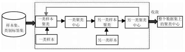
为了建立适用于不平衡数据分类的模糊规则前件参数学习方法, 同时也为了提高所得模糊规则的准确性和可解释性, 本文提出了竞争贝叶斯模糊聚类(BFCCL). BFCCL聚类的出发点为:在聚类过程中, 一类样本会对另一类别的聚类中心产生排斥的影响, 特别是在不同类别样本的重叠区域, 一方面, 聚类中心受到本类别样本的吸引而靠近该区域; 另一方面, 聚类中心受到异类别样本的排斥而远离该区域.这种排斥关系可表现为不同类别的聚类中心在样本叠加区域的一种竞争学习关系.当样本重叠区域的重叠密度越大时, 属于不同类别的聚类中心之间的竞争力也就越大.本文将这思想融入到BFC贝叶斯概率模型中, 在样本的类别标签已知的前提下, 采用在两类样本交替循环执行的策略, 两类的聚类中心分别作为已知数据, 参与到另一类样本聚类的过程中, 起到聚类中心竞争学习的作用.两类聚类中心交替影响, 直至两类聚类中心都处于稳定状态. BFCCL聚类的构造原理示意图如图 1所示.
2.2 目标函数的构造和参数学习方法
由图 1可知, BFCCL聚类通过两类交替循环的策略实现数据集的最佳模糊划分, 本节以某一类样本为例, 重点阐述BFCCL聚类模型的目标函数和参数学习方法.设给定某一类样本集${{\pmb X}}=\{{{{{\pmb x}}}_{1}}, {{{{\pmb x}}}_{2}}, \cdots, {{{{\pmb x}}}_{N}}\}$, 聚类数为$C_{1}$, 假设另一类样本的聚类中心已知, 为${\pmb Z}={{\left[{{\pmb{z}}_{1}}, {{\pmb{z}}_{2}}, \cdots, {{\pmb{z}}_{{{{c}}_{2}}}} \right]}^{\rm T}}$, 聚类数为$C_{2}$.基于BFC模型的贝叶斯概率模型, 样本${{\pmb X}}$服从正态分布, 并且每个样本具有独立的概率分布, 因此BFCCL聚类中样本集${{\pmb X}}$中数据和参数的联合概率模型可表示为式(13).
$ p({{\pmb X}}, {\pmb{Z}}, {\pmb{U}}, {\pmb{Y}})=p({{\pmb X}}, {\pmb{Z}}|{\pmb{U}}, {\pmb{Y}})p({\pmb{U}}|{\pmb{Y}})p({\pmb{Y}}) \propto \exp\\\Big\{ -\frac{1}{2}\Big(\sum\limits_{n=1}^{N}{\sum\limits_{c=1}^{{{C}_{1}}}{u_{nc}^{m}||{{{{\pmb x}}}_{n}}- {{\pmb{y}}_{c}}|{{|}^{2}}+\sum\limits_{n=1}^{N}{\sum\limits_{c= {{C}_{1}}+1}^{{{C}_{1}}+{{C}_{2}}}{u_{nc}^{m}||{{\pmb x}}}_{n}}-}} \nonumber\\ {{\pmb{z}_{c}|{|}^{2}}\Big)} \Big\}\times \left[\prod\limits_{n=1}^{N}{\prod\limits_{c=1}^{{{C}_{1}}+{{C}_{2}}}{u_{nc}^ {{{\alpha }_{c}}-1}\times \exp\left\{ -\frac{1}{2}\sum\limits_{c=1}^{{{C}_{1}}}{{{( {{\pmb{y}}_{c}}-{{{\pmb\mu }}_{y}})}^{\rm T}}\sum\nolimits_{y}^{-1}{({{\pmb{y}}_{c}}-{{\pmb\mu }}_{y}})} \right\}} }\right] $
(13) 其中, 样本集${{\pmb X}}$和另一类聚类中心矩阵$\pmb{Z}$为模型的已知数据, 需构建的聚类中心矩阵${\pmb Y=}{{\left[{{\pmb{y}}_{1}}, {{\pmb{y}}_{2}}, \cdots, {{\pmb{y}}_{{{c}_{1}}}} \right]}^{\rm T}}$和模糊隶属度矩阵${\pmb U}$是模型的参数.通过对上式取对数, 可得BFCCL模型的目标函数:
$ \begin{eqnarray} &&J({{\pmb X}}, {\pmb{Z}}, {\pmb{U}}, {\pmb{Y}})=\sum\limits_{n=1}^{N}{\sum\limits_{c=1}^{{{C}_{1}}}{u_{nc}^{m}||{{{{\pmb x}}}_{n}} -{{\pmb{y}}_{c}}|{{|}^{2}}+}}\nonumber\\ &&\qquad\sum\limits_{n=1}^{N}{\sum\limits_{c={{C}_{1}}+1}^{{{C}_{1}}+{{C}_{2}}}{u_{nc}^{m}||{{{{\pmb x}}}_{n}} -{{\pmb{z}}_{c}}|{{|}^{2}}}}-\nonumber \\ &&\qquad2\sum\limits_{n=1}^{N}{\sum\limits_{c=1}^{{{C}_{1}}+{{C}_{2}}}{({{\alpha }_{c}}-1)\log ({{u}_{nc}})}}+ \nonumber\\ &&\qquad\sum\limits_{c=1}^{{{C}_{1}}}{{{({{\pmb{y}}_{c}}-{{{\pmb\mu }}_{y}})}^{\rm T}}\sum\nolimits_{y}^{-1}{({{\pmb{y}}_{c}}-{{{\pmb\mu }}_{y}})}} \end{eqnarray} $
(14) 结合上述联合概率模型(13) 和目标函数式(14), 给出如下分析和说明:
1) 不同于常规聚类方法不考虑样本所带的标签信息, BFCCL模型目标函数中的前2项表示出不同类别的聚类中心间的竞争关系.在另一类样本的聚类中心已知的前提下, 待求聚类中心必然会与这些已知聚类中心对模糊隶属度产生"竞争"关系, 这种竞争关系可理解为不同类别聚类中心间的相互排斥关系; 同时这种竞争关系能保证空间划分的清晰性和增强所得模糊规则的准确性和可解释性.
2) 由图 1可知, 为了获得整个数据集的最佳空间划分, 需在正负类样本上采取交替循环的策略来求解式(13) 的最大后验值.在循环的过程中两类聚类中心相互影响, 直至两类的聚类中心处于稳定状态.
3) 模糊指数$m$起到调节竞争力强弱的作用, $m$的值越大, 聚类中心间的竞争力就越弱; 反之, $m$的值越小, 聚类中心间的竞争力就越强.
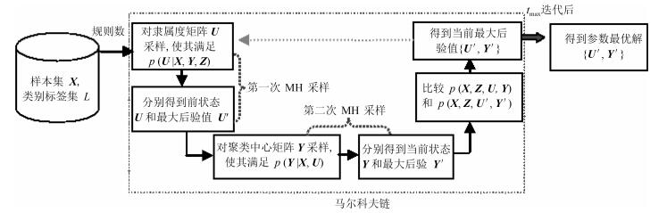
为了获得最优模糊隶属度矩阵$\pmb U$和聚类中心矩阵$\pmb Y$, BFCCL通过先后两次使用Metropolis-Hastings (MH)采样[27]构造一条Markov链来获得模型参数的最大后验值, 其参数的学习过程如图 2所示.从图 2可知, 该Markov链的第$n$次迭代的过程可主要分为3步:
步骤1. 在给定样本和聚类中心的情况下, 使用Metropolis-Hastings方法对模糊隶属度${{\pmb{u}}_{n}}$进行采样:
a) 由Dirichlet分布产生一个新的模糊隶属度值${\pmb u}_{n}'$, 并将Dirichlet分布的参数${\pmb\alpha }$设置为${\pmb\alpha }={{ {\bf 1}}_{C}}$, 即
$ \begin{eqnarray} {\pmb u}_{n}'\sim {\rm Dirichlet}( {\pmb\alpha }={{ {\bf 1}}_{C}}) \end{eqnarray} $
(15) b) 计算采样值$ {\pmb u}_{n}'$的接受概率:条件分布$p({\pmb U}|{{\pmb X}}, {\pmb Z}, {\pmb Y})$在样本和聚类中心已知的情况下与联合分布$p({{\pmb X}}, {\pmb Z}, {\pmb U}, {\pmb Y})$成比例, 同时也与条件分布$p({{\pmb X}}, {\pmb U}|{\pmb Y}, {\bf Z})$成比例.因此, 接受概率${{a}_{{\pmb u}}}$的计算公式可写成以下形式:
$ \begin{eqnarray} {{a}_{{U}}}=\min \left\{ 1, \frac{p({{\pmb X}_n} , {{{{\pmb{u}}}}_{n}'}|{\pmb Y}, {\pmb Z})}{p({{\pmb x}_n}, {{{\pmb u}}_{n}}|{\pmb Y}, {\pmb Z})} \right\} \end{eqnarray} $
(16) 其中, ${{{\pmb u}}_{n}}$表示样本${{{{\pmb x}}}_{n}}$当前状态的模糊隶属度, $p({{{{\pmb x}}}_{n}}, {{{\pmb u}}_{n}}|{\pmb Y}, {\pmb Z})$的计算式如式(17).
$ \begin{eqnarray} p({{{{\pmb x}}}_{n}}, {{{\pmb u}}_{n}}|{\pmb Y}, {\pmb Z})=p({{{{\pmb x}}}_{n}}|{{{\pmb u}}_{n}}, {\pmb Y}, {\pmb Z})p ({{{\pmb u}}_{n}}|{\pmb Y}, {\pmb Z})= \\ \qquad\prod\limits_{c=1}^{{{C}_{1}}}{\mathcal{N}({{{{\pmb x}}}_{n}}|{{{\pmb y}}_{c}}, u_{nc}^{m})u_{nc}^{-m\frac{D}{2}} \prod\limits_{c={{C}_{1}}+1}^{{{C}_{1}}+{{C}_{2}}}{\mathcal{N}({{{{\pmb x}}}_{n}}| {{{\pmb z}}_{c}}, u_{nc}^{m})u_{nc}^{-m\frac{D}{2}}}\rm {Dirichlet}({{{\pmb u}}_{n}}|{\pmb \alpha })} \propto\\ \prod\limits_{c=1}^{{{C}_{1}}}{\exp\Big(-\frac{1}{2}u_{nc}^{m}||{{{{\pmb x}}}_{n}}-{{{\pmb y}}_{c}}|{{|}^{2}}\Big)u_{nc}^{{{\alpha }_{c}}-1}\prod\limits_{c={{C}_{1}}+1}^{{{C}_{1}}+{{C}_{2}}}{\exp\Big(-\frac{1}{2}u_{nc}^{m}||{{{{\pmb x}}}_{n}}-{{{\pmb z}}_{c}}|{{|}^{2}}\Big)}\ }u_{nc}^{{{\alpha }_{c}}-1} \end{eqnarray} $
(17) 值得注意的是, 通过采样方式获得的新采样值${\pmb u}_{n}'$其分布和当前样本无关, 且${\pmb u}_{n}'/{\pmb u}_{n}$在不同时刻状态独立, 因此判决函数${{a}_{{\pmb u}}}$不需要进行Hasting校验.
c) 比较$p({{{{\pmb x}}}_{n}}, {{{\pmb {u}}}_{n}'}|{\pmb Y}_{{}}^{*}, {\pmb Z})$和$p({{{{\pmb x}}}_{n}}, {\pmb u}_{n}^{*}|{\pmb Y}_{{}}^{*}, {\pmb Z})$, 其中${\pmb Y}_{{}}^{*}$和${\pmb u}_{n}^{*}$分别是当前聚类中心$Y$和隶属度${\pmb u}_{n}^{{}}$的最优值.如果$p({{{{\pmb x}}}_{n}}, {{{\pmb{u}}}_{n}'}|{\pmb Y}_{{}}^{*}, {\pmb Z})$大于$p({{{{\pmb x}}}_{n}}, {\pmb u}_{n}^{*}|{\pmb Y}_{{}}^{*}, {\pmb Z})$, 那么${\pmb u}_{n}'$替换${\pmb u}_{n}^{*}$.
步骤2. 为了获得聚类中心矩阵$\pmb Y$的最优值, BFCCL使用Metropolis-Hastings方法对$\pmb Y$进行采样:
a) 通过以下正态分布对聚类中心进行采样, 即
$ {{{\pmb y}}}_{c}'\sim\mathcal{N}({{{\pmb y}}_{c}}, \frac{1}{\sigma }\sum{_{y}}) $
(18) 其中该正态分布的均值为当前聚类中心${\pmb y}_{c}$, $\sum{_{y}}$为样本的协方差矩阵, 参数$\sigma $用来控制生成的聚类中心的紧度.
b) 计算采样值${{{{\pmb y}}}_{c}'}$的接受概率:对于固定的一类样本${{\pmb X}}$, 隶属度矩阵${\pmb U}$和另一类聚类中心矩阵${\pmb Z}$, $p({\pmb Y}|{{\pmb X}}, ~{\pmb U}, ~{\pmb Z})$与$p({\pmb Y}, ~{{\pmb X}}, ~{\pmb U}, {\pmb Z})$和$p({{\pmb X}}, ~{\pmb U}, ~ {\pmb Y})$成比例, 同时也与$p({{\pmb X}}, ~{\pmb Y}|{\pmb U})$成比例.因此, 这里只需估计每一个样本${{{\pmb Y}}}_{c}'$的条件概率$p({{\pmb X}}, {{{\pmb y}}_{c}}|{\pmb U})$.其接受概率${{a}_{{\pmb y}}}$可表达式为
$ \begin{eqnarray} {{a}_{{\pmb y}}}=\min \left\{ 1, \frac{p({{\pmb X}}, {{{\pmb{y}}}}_{c}'|{\pmb U})}{p({{\pmb X}}, {{{\pmb y}}_{c}}|{\pmb U})} \right\} \end{eqnarray} $
(19) 由于新产生的状态独立于其他聚类中心, 因此, 条件分布$p({{\pmb X}}, {{{\pmb y}}_{c}}|{\pmb U})$的计算式可以写成:
$ \begin{align} p({{\pmb X}}, {{{\pmb y}}_{c}}|{\pmb U})= &p({{\pmb X}}\!\!|\!\!{\pmb U}, {{{\pmb y}}_{c}})p({{{\pmb y}}_{c}})\propto ~~~~~~~~~~~~~\nonumber\\ &\exp \left\{ -\frac{1}{2}\sum\limits_{n=1}^{N}{u_{nc}^{m}||{{{{\pmb x}}}_{n}}- {{{\pmb y}}_{c}}|{{|}^{2}}} \right\}\times \nonumber\\ &\exp \left\{ -\frac{1}{2}{{({{{\pmb y}}_{c}}-{{\pmb\mu }_{y}})}^{\rm {T}}} \sum\nolimits_{y}^{-1}{({{{\pmb y}}_{c}}-{{\pmb\mu }_{y}})} \right\} \end{align} $
(20) 因为${{{\pmb{y}'}}_{c}}$服从高斯分布满足对称性, 式(19) 也无需进行Hastings校验.
c) 比较$p({{\pmb X}}, ~{\pmb y}_{c}'|{\pmb U}_{{}}^{*})$和$p({{\pmb X}}, ~{\pmb y}_{c}^{*}|{\pmb U}_{{}}^{*})$, 其中${\pmb U}_{{}}^{*}$和${\pmb y}_{c}^{*}$分别是模糊隶属度矩阵$U$和聚类中心${\pmb y}_{c}^{{}}$的最优值.如果$p({{\pmb X}}, ~{\pmb y}_{c}'|{\pmb U}_{{}}^{*})$大于$p({{\pmb X}}, ~{\pmb y}_{c}^{*}|{\pmb U}_{{}}^{*})$, 那么${\pmb y}_{c}'$替换${\pmb y}_{c}^{*}$.
步骤3. 根据式(13) 计算$p({{\pmb X}}, ~{{{\pmb U}}^{*}}, ~{{{\pmb Y}}^{*}}, ~{\pmb Z})$的值并与当前$p({{\pmb X}}, ~{\pmb U}, ~{\pmb Y}, ~{\pmb Z})$的值进行比较, 若$p({{\pmb X}}, ~{\pmb U}, ~{\pmb Y}, ~{\pmb Z})>p({{\pmb X}}, ~{{{\pmb U}}^{*}}, ~{{{\pmb Y}}^{*}}, ~{\pmb Z})$, 则用$\{{\pmb U}, ~{\pmb Y}\}$替换当前的$\{{{{\pmb U}}^{*}}, ~{{{\pmb Y}}^{*}}\}$.
2.3 BFCCL聚类算法
本文将研究重点置于最基本的二元分类问题.结合图 1所示的BFCCL聚类构造原理示意图和第2.2节的内容, 本节给出BFCCL聚类算法在整个数据集上实施的具体步骤, 见算法1.设全体样本$\{{{{{\pmb x}}}_{1}}, {{{{\pmb x}}}_{2}}, \cdots, {{{{\pmb x}}}_{N}}\}$和其对应的类别标签$\{{{l}_{1}}, {{l}_{2}}, \cdots, {{l}_{N}}\}~({{l}_{i}}\in \{-1, +1\}, ~i=1, 2, \cdots, N)$, 其中${{{{\pmb X}}}_{1}}=\{{{{{\pmb x}}}_{1}}, {{{{\pmb x}}}_{2}}, \cdots, {{{{\pmb x}}}_{{{N}_{1}}}}\}$和${{{{\pmb X}}}_{2}}=\{{{{{\pmb x}}}_{{{N}_{1}}+1}}, {{{{\pmb x}}}_{{{N}_{1}}+2}}, \cdots, {{{{\pmb x}}}_{N}}\}$分别表示正负两类样本.为了获得全体样本的最佳空间划分, 需在正负类上采取交替循环的策略来执行式(13).两类聚类中心交替影响, 直至两类的聚类中心处于稳定状态.
BFCCL聚类采取两类样本交替循环执行的策略来获得聚类中心和模糊隶属度的最优解, BFCCL聚类中单次循环的时间复杂度主要在于步骤2的执行, 而步骤2又由两部分构成:计算模糊隶属度矩阵$\pmb U$和聚类中心矩阵$\pmb Y$, 前者的时间复杂度由式(17) 产生, 为O$(NCD+C{{D}^{2}})$; 后者的时间复杂度由式(20) 产生, 为O$(C{{D}^{2}})$.因此, BFCCL聚类算法执行的时间复杂度为O$({{v}_{\rm {max}}}{{t}_{\rm {max}}}(NCD+C{{D}^{2}}))$, 其中${t}_{\rm {max}}$和${v}_{\rm {max}}$分别是算法正负类交替迭代和Metropolis-Hastings采样方法中迭代的次数.另外, 实验中一般可将式(18) 中的协方差矩阵设为对角阵, 此时, 算法1的复杂度可减少至O$({{v}_{\rm {max}}}{{t}_{\rm {max}}}NCD)$.可见, BFCCL聚类算法运行的时间效率与样本的分布和结构有关, 为了在一定程度上提高本文方法的执行效率, 可以采用KPCA等降维方法对样本进行相应的预处理, 或者采用正交三角(QR)等分解法对式(20) 中的协方差矩阵进行变换处理.
算法1. BFCCL聚类算法
输入. 正负两类数据集${{{{\pmb X}}}_{1}}$和${{{{\pmb X}}}_{2}}$, 模糊指数$m$, 正、负类样本的聚类个数分别为${C}^{(1)}$和${C}^{(2)}$, MH采样最大迭代次数${v}_{\rm {max}}$, 两类交替循环最大迭代次数${{t}_{\rm {max}}}$, 误差阈值$\varepsilon $;
输出. 模糊隶属度矩阵${\pmb U}_{{}}^{(1)*}$, ${\pmb U}_{{}}^{(2)*}$和聚类中心${{{\pmb Y}}^{(1)*}}, {{{\pmb Y}}^{(2)*}}$.
初始化. 在数据集${{{{\pmb X}}}_{1}}$和${{{{\pmb X}}}_{2}}$分别计算正负类样本的均值${\bf \mu }_{y}^{(1)}$, ${\bf \mu }_{y}^{(2)}$和协方差$\sum{_{y}^{(1)}}$, $\sum{_{y}^{(2)}}$; 在数据集${{{{\pmb X}}}_{1}}$和${{{{\pmb X}}}_{2}}$分别进行两类模糊隶属度矩阵${\pmb U}^{(1)}$和${\pmb U}^{(2)}$进行初始化, 其中${\pmb U}^{(1)}$矩阵中的元素${\pmb u}_{n}^{(1)}\sim{\ }\rm {Dirichlet}({\pmb \alpha }={{{\bf 1}}_{C}})$, ${\pmb U}^{(2)}$矩阵中的元素${\pmb u}_{n}^{(2)}\sim{\ }\rm {Dirichlet}({\pmb \alpha }={{{\bf 1}}_{C}})$, ($n=1, \cdots, N, \ C={C}^{\left( 1 \right)}+{C}^{\left( 2 \right)}$); 在数据集${{{{\pmb x}}}_{1}}$和${{{{\pmb x}}}_{2}}$分别对两类聚类中心矩阵${\pmb Y}^{(1)}$和${\pmb Y}^{(2)}$进行初始化, 其中${\pmb Y}^{(1)}$矩阵中的元素${\pmb y}_{c}^{(1)}$: ${\pmb y}_{c}^{(1)}\sim{\ }\mathcal{N}({\bf \mu }_{y}^{(1)}, \sum{_{y}^{(1)}}\rm{) (}c=1, \cdots, {{C}^{\left( 1 \right)}})$, ${\pmb Y}^{(2)}$矩阵中的元素${\pmb y}_{c}^{(2)}\sim {\ }\mathcal{N}({\bf \mu }_{y}^{(2)}\sum{_{y}^{(2)}})\ (c=1, \cdots, {{C}^{\left( 2 \right)}})$; 在数据集${{{{\pmb X}}}_{1}}$和${{{{\pmb X}}}_{2}}$分别对模糊隶属度矩阵和聚类中心矩阵的最大后验值进行初始化, ${\pmb U}_{{}}^{(1)*}= {\pmb U}(1)$, ${\pmb U}_{{}}^{(2)*}= {\pmb U}(2)$, ${{{\pmb Y}}^{(1)*}}={{{\pmb Y}}^{\left( 1 \right)}}, {{{\pmb Y}}^{(2)*}}={{{\pmb Y}}^{(2)}}$;
For $v=0$ to $v_{\rm {max}}$
For $t=1$ to $t_{\rm {max}}$
步骤1. 令${{\pmb X}}={{{{\pmb X}}}_{1}}$, ${\pmb Z}={{{\pmb Y}}^{(2)*}}(v)$, ${\pmb U}_{{}}^{*}={\pmb U}_{{}}^{(1)*}$, ${C}_{1} = {C}^{(1)}$, ${C}_{2} = {C}^{(2)}$
步骤2.
For $n=1$ to size(${{\pmb X}}$)
{步骤2.1. 根据式(15) 得到隶属度${\pmb u}_{n}'$;
步骤2.2. 根据式(16) 计算$p({{{{\pmb x}}}_{{n}}}, {{{\pmb {u}}}_{n}'}|{\pmb Y}, {\pmb Z})$和$p({{{{\pmb x}}}_{{n}}}, {{{\pmb u}}_{n}}|{\pmb Y}, {\pmb Z})$, 并以式(17) 的概率接受${{{\pmb u}}_{n}}\leftarrow {{{\pmb {u}}}_{n}'}$;
步骤2.3. 根据式(17), 如果$p({{{{\pmb x}}}_{n}}, {{{\pmb {u}}}_{n}'}|{\pmb Y}_{{}}^{*}, {\pmb Z}) < p$ $({{{{\pmb x}}}_{n}}, {\pmb u}_{n}^{*}|{\pmb Y}_{{}}^{*}, ~{\pmb Z})$, 那么${\pmb u}_{n}^{*}\leftarrow {\pmb u}_{n}'$;
步骤2.4. 如果$n>N$, 则转至步骤2.5;否则, 置$n = n+1$, 并返回步骤2.1};
End $n$
For $c=1$ to size(${C}_{1}$)
{步骤2.5. 根据式(18) 采样新的聚类中心${{{{\pmb y}}}_{c}'}$;
步骤2.6. 以式(19) 的概率${{a}_{{\pmb y}}}$接受${\pmb y}_{c}^{{}}\leftarrow {{{{\pmb y}}}_{c}'}$;
步骤2.7. 根据式(20), 如果$p({{\pmb x}}, ~{\pmb y}_{c}'|{{{\pmb U}}^{*}})>p({{\pmb x}}, ~{\pmb y}_{c}^{*}|{{{\pmb U}}^{*}})$, 那么${\pmb y}_{c}^{*}\leftarrow {\pmb y}_{c}'$;
步骤2.8. 如果$c> {C}_{1}$, 则转至步骤2.9;否则, 置$c=c+1$, 返回步骤2.6;
步骤2.10. 如果$p({{\pmb X}}, ~{{{\pmb U}}^{*}}, ~{{{\pmb Y}}^{*}}, ~{\pmb Z})>p({{\pmb X}}, {\pmb U}, {\pmb Y}, {\pmb Z})$, 那么${{{\pmb U}}^{*}}\leftarrow {\pmb U}$, ${{{\pmb Y}}^{*}}\leftarrow {\pmb Y}$; }
End $c$
步骤2.10. 如果$t >{{t}_{\rm {max}}}$, 则将${\pmb U}_{{}}^{*}$和${{{\pmb Y}}^{*}}$分别设置为当前样本的模糊隶属度矩阵和聚类中心矩阵的最大后验值并转至步骤3;否则, 转至步骤2.1;
步骤3. 令${{\pmb X}}={{{{\pmb X}}}_{2}}$, ${\pmb Z}={{{\pmb Y}}^{(1)*}}(v)$, ${\pmb U}_{{}}^{*}={\pmb U}_{{}}^{(2)*}$, ${C}_{1} = {C}^{(2)}$, ${C}_{2} = {C}^{(1)}$
步骤4. 转向步骤2
End $t$
步骤5. 如果$\left| {{{\pmb Y}}^{(1)*}}(v)-{{{\pmb Y}}^{(1)*}}(v-1) \right|\le \varepsilon $或者$v > v_{\rm {max}}$, 则算法停止并输出${\pmb U}_{{}}^{(1)*}$, ${\pmb U}_{{}}^{(2)*}$和${{{\pmb Y}}^{(1)*}}, {{{\pmb Y}}^{(2)*}}$; 否则, 置$v = v+1$, 转至步骤5.
End $v$.
3. 用于不平衡数据分类的0阶TSK型模糊系统(0-TSK-IDC)
对于给定的样本及其类别标签$\{{{{{\pmb x}}}_{i}}, {{l}_{i}}\}_{i=1}^{N}$由算法1完成BFCCL聚类后, 得到的每一个聚类对应于0-TSK-IDC模糊系统中的一条模糊规则.同时分别属于两类样本的模糊隶属度矩阵${\pmb U}_{{}}^{(1)*}$, ${\pmb U}_{{}}^{(2)*}$和聚类中心矩阵${{{\pmb Y}}^{(1)*}}, {{{\pmb Y}}^{(2)*}}$为构建高斯隶属度函数(式(4))提供了依据, 高斯隶属度函数的方差${{{\pmb \delta }}^{(1)}}$和${{{\pmb \delta }}^{(2)}}$可由下式计算得到:
$ \begin{eqnarray*} ~\delta _{c, i}^{(1)}=\frac{h\sum\limits_{j=1}^{{{N}_{1}}}{{{u}_{jc}}{{({{x}_{ji}}-y_{c, i}^{(1)})}^{2}}}}{ \sum\limits_{j=1}^{{{N}_{1}}}{{{u}_{jc}}}}, ~\begin{array}{ll}i=1, 2, \cdots, D\\c=1, 2, \cdots, {{C}^{\left( 1 \right)}}\\{{{{\pmb x}}}_{j}}\in {{{{\pmb X}}}_{1}}\end{array} \end{eqnarray*} $
(21) $ \begin{eqnarray*} \delta _{c, i}^{(2)}=\frac{h\sum\limits_{j={{N}_{1}}+1}^{N}{{{u}_{jc}}{{({{x}_{ji}}-y_{c, i}^{(2)})}^{2}}}} {\sum\limits_{j={{N}_{1}}+1}^{N}{{{u}_{jc}}}}, ~\begin{array}{ll}i=1, 2, \cdots, D\\ c=1, 2, \cdots, {{C}^{\left( 2 \right)}}\\{{{{\pmb x}}}_{j}}\in {{{{\pmb X}}}_{2}}\end{array} \end{eqnarray*} $
(22) 当模糊规则的前件参数(矩阵${\pmb Y}~({\pmb Y}={{[{{{\pmb Y}}^{(1)*}}, {{{\pmb Y}}^{(2)*}}]}^{\rm {T}}}$)和${\pmb \delta }({\pmb \delta }={{[{{{\pmb \delta }}^{(1)}}, {{{\pmb \delta }}^{(2)}}]}^{\rm {T}}})$确定后, 使用式(3) ~ (5) 可将原始数据集$\{{{{{\pmb x}}}_{i}}, {{l}_{i}}\}_{i=1}^{N}$映射至特征空间形成新的数据集$\left\{ d({{{{\pmb x}}}_{i}}), \ {{l}_{i}} \right\}_{i=1}^{N}$, 其中$d({{{{\pmb x}}}_{i}})$可写成以下形式:
$ \begin{eqnarray} d({{{{\pmb x}}}_{i}})={{[{{\tilde{\mu }}_{1}}({{{{\pmb x}}}_{i}}), {{\tilde{\mu }}_{2}}({{{{\pmb x}}}_{i}}), \cdots, {{\tilde{\mu }}_{{{C}^{\left( 1 \right)}}+{{C}^{\left( 2 \right)}}}}({{{{\pmb x}}}_{i}})]}^{\rm T}} \end{eqnarray} $
(23) 令${{{\pmb p}}_{0}}={{[p_{0}^{1}, p_{0}^{2}, \cdots, p_{0}^{{{C}^{\left( 1 \right)}}+{{C}^{\left( 2 \right)}}}]}^{\rm T}}$, 0-TSK-IDC模糊系统的后件参数学习转化为求解规则后件${\pmb p}_0$的线性问题, 即
$ \begin{eqnarray} f({{{{\pmb x}}}_{i}})={{{\pmb p}}_{0}}^{\rm {T}}d({{{{\pmb x}}}_{i}})\left\{ \begin{gathered} \ge 0, \ \ \ {{{{\pmb x}}}_{i}}\in {{{{\pmb X}}}_{1}} \\ < 0, \ \ \ {{{{\pmb x}}}_{i}}\in {{{{\pmb X}}}_{2}} \\ \end{gathered} \right.\ \end{eqnarray} $
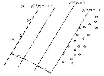
(24) 传统分类面的大间隔的策略是达到两类间距离的最大化, 但这种分类面在处理不平衡分类问题中易向少数类发生偏移.为纠正分类面的偏移, 本文寻找的分类面在达到两类间距离的最大化的同时, 保证少数类到分类面的距离不得小于多数类到分类面的距离, 其示意图如图 3所示.因此后件参数的学习问题可用以下最优化问题来表示:
$ \begin{eqnarray} \underset{\rho, {{{\pmb p}}_{0}}, \xi }{\mathop{\min }} \ \ \frac{1}{2}{\pmb p}_{0}^{\rm T}{{{\pmb p}}_{0}}-v{{\rho }^{2}}+{{\lambda }_{1}}\sum\limits_{i=1}^{{{N}_{1}}}{{{\xi }_{i}}}+{{\lambda }_{2}}\sum\limits_{j={{N}_{1}}+1}^{{{N}_{{}}}}{{{\xi }_{j}}} ~~~~~~~~~ \nonumber\\ {\rm s. t}.\ \ {{{\pmb p}}_{0}}^{\rm T}d({{{{\pmb x}}}_{i}})\ge 1\ +{{\rho }^{2}}\ -{{\xi }_{i}}\, \ i=1, 2, \cdots, {{N}_{1}} ~~~~\nonumber\\ -{{{\pmb p}}_{0}}^{\rm T}d({{{{\pmb x}}}_{j}})\ge 1-\ {{\xi }_{j}}\, \ j={{N}_{1}}+1, {{N}_{1}}+2, \cdots, N \end{eqnarray} $
(25) 其中, $v, {{\lambda }_{1}}$和${{\lambda }_{2}}$为3个正常数, 且${{{\lambda }_{1}}}/{{{\lambda }_{2}}}={{{N}_{2}}}/{{{N}_{1}}}={(N-{{N}_{1}})}/{{{N}_{1}}}$.
求解式(25) 可以利用Lagrange技巧, 引入非负的Lagrange因子${{\pmb \alpha} }$, $L({{{\pmb p}}_{0}}, \rho, \xi )$方程的各变量求偏导数, 并令各偏导方程为零, 上述最优化问题可以转换成对偶形式:
$ \begin{eqnarray} && \underset{{\pmb \alpha }}{\mathop{\min }} \ -\frac{1}{2}{{{\pmb \alpha }}^{\rm T}}{\pmb K}{\pmb \alpha } \nonumber\\ && \rm{s}\rm{. t}.\ \sum\limits_{i=1}^{{{N}_{1}}}{{{\alpha }_{i}}}=v\ \nonumber\\ && \ \ \ \ \sum\limits_{j={{N}_{1}}}^{N}{{{\alpha }_{j}}}=v \nonumber\\ &&0\le {{\alpha }_{i}}\le {{\lambda }_{1}}, ~ i=1, \cdots, {{N}_{1}} \nonumber\\ &&0\le {{\alpha }_{j}}\le {{\lambda }_{2}}, ~ j={{N}_{1}}+1, \cdots , N \end{eqnarray} $
(26) 其中, ${\pmb K}={{[{{k}_{ij}}]}_{N\times N}}, {{k}_{ij}}={{l}_{i}}{{l}_{j}}d{{({{{{\pmb x}}}_{i}})}^{\rm T}}d({{{{\pmb x}}}_{j}})$.根据优化理论, 当且仅当${\pmb K}(\cdot )$为Mercer核时式(26) 为二次凸规划, 求得的解是全局最优解.这里, 证明其为Mercer核.
引理1[28]. 令${{\pmb x}}$是${{{\pmb R}}^{n}}$上的一个紧集, ${\pmb K}({{\pmb x}}, {{\pmb x}})$是Mercer核当且仅当${\pmb K}({{\pmb x}}, {{\pmb x}})$是${{\pmb X}}$×${{\pmb X}}$上连续对称函数且关于任意的${{{{\pmb x}}}_{1}}, \cdots, {{{{\pmb x}}}_{l}}\in {{\pmb X}}$的Gram矩阵半正定.
定理1. 如果模糊系统中前件的模糊隶属函数${{\tilde{\mu }}_{k}}({{\pmb x}})$是连续函数, 则式(26) 的核函数$\pmb K$是Mercer核.
证明. 根据式(26) 的定义, ${\pmb K}={{[{{k}_{ij}}]}_{N\times N}}, {{k}_{ij}}={{l}_{i}}{{l}_{j}}d{{({{{{\pmb x}}}_{i}})}^{\rm {T}}}d({{{{\pmb x}}}_{j}})$, 容易看出${\pmb K}$是一个实对称矩阵.其次, 对任意的${{\alpha }_{1}}, \cdots, {{\alpha }_{N}}\in \bf{R}$, 由式(23), 有$\sum_{i, j}^{N}{{{\alpha }_{i}}{{\alpha }_{j}}{{k}_{ij}}}=\sum_{i, j}^{N}{{{\alpha }_{i}}{{\alpha }_{j}}}{{l}_{i}}{{l}_{j}}d{{({{{{\pmb x}}}_{i}})}^{\bf {T}}}d({{{{\pmb x}}}_{j}})={{\left\| \sum_{i=1}^{N}{\sum_{k=1}^{_{{{C}^{\left( 1 \right)}}+{{C}^{\left( 2 \right)}}}}{{{\alpha }_{i}}{{l}_{i}}{{{\tilde{\mu }}}_{k}}({{{{\pmb x}}}_{i}})}} \right\|}^{2}}\ge 0$且${{\tilde{\mu }}_{k}}({{\pmb x}})$是连续函数, 因此核函数$\pmb K$是Mercer核.
因此, 设${{{\pmb \alpha }}^{*}}={{[\alpha _{1}^{*}, \cdots, \alpha _{N}^{*}]}^{\rm {T}}}$为式(26) 的解, 则0-TSK-IDC的后件参数$p_{0}^{k}$为
$ \begin{eqnarray} p_{0}^{k}=\sum\limits_{i=1}^{N}{{{l}_{i}}\alpha _{i}^{*}{{{\tilde{\mu }}}_{k}}({{{{\pmb x}}}_{i}})} \end{eqnarray} $
(27) 最终, 0-TSK-IDC模糊系统的决策函数$F({{\pmb x}}$)可表示为
$ F({{\pmb x}})={\rm {sgn}}({{{\pmb p}}_{0}}^{\rm {T}}d({{\pmb x}})) $
(28) 根据上文的分析和推导, 0-TSK-IDC使用BFCCL算法得到准确性和可解释性强的规则前件参数, 规则后件参数着眼于分类面的偏移纠正.这里总结出0-TSK-IDC模糊系统的具体训练步骤, 具体如下:
算法2. 0-TSK-IDC模糊系统
输入. 数据集$\{{{{{\pmb x}}}_{i}}, {{l}_{i}}\}_{i=1}^{N}$, 模糊规则数($ C^{(1)} + C^{(2)}$), 模糊指数$m$, 尺度参数$h$, MH采样最大迭代次数$v_{\rm {max}}$, 两类交替循环最大迭代次数${{t}_{\rm {max}}}$, 误差阈值$\varepsilon $, 调节参数$v$, 正则化参数${{\lambda }_{1}}$和${{\lambda }_{2}}$;
输出. 分类决策函数$F({{\pmb x}})$.
步骤1. 根据算法1得到隶属度矩阵${\pmb U}_{{}}^{(1)*}$, ${\pmb U}_{{}}^{(2)*}$和聚类中心矩阵${{{\pmb Y}}^{(1)*}}, ~{{{\pmb Y}}^{(2)*}}$;
步骤2. 由式(22) 计算高斯隶属度函数的方差矩阵${{{\pmb \delta }}^{(1)}}$和${{{\pmb \delta }}^{(2)}}$;
步骤3. 由式(3) ~ (5) 0-TSK-IDC将原始数据集$\{{{{{\pmb x}}}_{i}}, {{l}_{i}}\}_{i=1}^{N}$映射至特征空间形成新的数据集$\left\{ d({{{{\pmb x}}}_{i}}), \ {{l}_{i}} \right\}_{i=1}^{N}$;
步骤4. 由式(26) 求解得到Lagrange因子${\pmb \alpha }$;
步骤5. 由式(27) 得到0-TSK-IDC的后件参数${{{\pmb p}}_{0}}$;
步骤6. 由式(28) 得到0-TSK-IDC的决策函数.
0-TSK-IDC模糊系统的时间复杂度主要集中在算法1和二次规划求极值问题上.二次规划问题的时间复杂度为O$(N^{3})$, 因此, 0-TSK-IDC模糊系统的时间复杂度为O$({{v}_{\rm {max}}}{{t}_{\rm {max}}}(NCD+C{{D}^{2}})+{{N}^{3}})$.本文使用SMO (Sequential minimal optimization)[20]等分解方法处理二次规划问题, 0-TSK-IDC模糊系统的时间复杂度降低至O$({{v}_{\rm {max}}}{{t}_{\rm {max}}}(NCD+C{{D}^{2}})+{{N}^{2}})$.
需要指出的是, 0-TSK-IDC模糊系统后件参数的学习策略与支持向量机(Support vector machine, SVM)[29]较为相似, 但这两种方法之间存在着本质差异, 0-TSK-IDC通过模糊规则完成特征空间的映射, 而SVM通过核函数直接将原始数据映射到特征空间上; 其次, 0-TSK-IDC分类决策函数中的参数同时也是模糊系统中模糊规则的参数, 其具有高度的语义性和可解释性, 这一特性是模糊系统特有的.
4. 实验结果与分析
4.1 实验设置
一般认为当少数类与多数类的样本比例低于1: 2时, 数据集具有不平衡特征.而现实生活中的医学诊断数据往往呈现出不平衡性, 本文的实验部分将利用人工Banana数据集[30]和4个UCI医学数据集[31] (基本信息见表 1)所示对BFCCL算法和0-TSK-IDC模糊系统进行验证和评价.依照不平衡数据分类问题中常用的设定方法, 实验中将少数类指定为正类, 将多数类指定为负类.
表 1 数据集的基本信息Table 1 The basic information of datasets数据集 正类样本数 负类样本数 正负类比例 属性个数 Banana dataset 600, 200, 100 1 500 2 : 5, 2 : 15, 1 : 15 2 Heart statlog 120, 60, 30, 20, 12 170 12 : 17, 6 : 17, 3 : 17, 2 : 17, 6 : 85 13 Breast wisconsin 241, 200, 150, 100, 40 458 241 : 458, 100 : 229, 75 : 229, 50 : 229, 20 : 229 10 Liver disorders 145, 100, 50, 20 200 29 : 40, 1 : 2, 1 : 4, 1 : 10 7 Haberman 81, 40, 25 225 9 : 25, 8 : 45, 1 : 9 3 本文的实验分成两个部分: 1) 0-TSK-IDC中规则前件参数学习分别使用BFCCL算法和BFC算法来进行性能的比较; 2) 0-TSK-IDC模糊系统与FS-FCSVM[32]、L2-TSK-FS[25]、Adaboost[33]和CS-SVM[34]算法进行性能的比较, 其中FS-FCSVM和L2-TSK-FS是基于模糊聚类的模糊系统; Adaboost和CS-SVM是处理不平衡数据分类的算法.为了验证本文所提的模糊规则的后件参数学习方法在不平衡分类问题上的有效性, 实验中还将0-TSK-IDC模糊系统与BFCCL-TSK-FS模糊系统进行了对比, BFCCL-TSK-FS模糊系统中规则前件参数的学习使用BFCCL聚类方法; 规则后件参数的学习使用与FS-FCSVM模糊系统相同的方法, 即标准的SVM算法.
实验参数设置如下: 0-TSK-IDC中最大迭代次数${{t}_{\rm {max}}} = 10^3$, ${{v}_{\rm {max}}}=10^3$, 式(19) 中的参数$\sigma $ = 3, 误差阈值$\varepsilon =10^{-5}$, 根据文献[35]模糊指数$m$取值为2, 此时物理意义最明确, 其他可人工设定的参数通过网格搜索的方式来确定, 尺度参数$h$取值为$\{{{0.2}^{2}}, {{0.4}^{2}}, \cdots, {{2}^{2}}\}$, 调节参数$v$取值为$\{{1}, {5}, \cdots, {30}\}$, 正则化参数${\lambda }_{2}$取值为$\{{10}^{-3}, \cdots, {10}^{3}\}$, ${{\lambda }_{1}}$的值根据${{\lambda }_{1}}={{\lambda }_{2}}{{N}_{2}}/{{N}_{1}}$来确定, 模糊规则数${C}_{1}$和${C}^{(2)}$取值均为$\{{1, 2, \cdots, 10}\}$.实验中, FS-FCSVM和L2-TSK-FS的规则前件由FCM聚类获得, 模糊指数$m$取值为2, 规则后件学习的正则化参数的设置与${{\lambda }_{2}}$相同. CS-SVM算法中的核函数采用高斯核, 核参数取值为$\{{10}^{-3}, \cdots, {10}^{3}\}$, 正则化参数的设置与${{\lambda }_{1}}$和${{\lambda }_{2}}$相同. Adaboost算法中设置弱分类器的个数为10. BFCCL-TSK-FS算法中BFCCL聚类的参数设置参照0-TSK-IDC, 其他参数的设置参照FS-FCSVM.
为了更好地呈现出不同程度的非平衡性对算法性能产生的影响, 本文采用$G-{\rm {mean}}$和$F-{\rm {measure}}$[36-37]两种评价准则来评价算法的分类性能:
$ G{\rm {-mean}}=\\~~ \sqrt{{\rm {Positive}}\ {\rm {Accuracy}}\times {\rm {Negative}}\ {\rm {Accuracy}}} $
(29) $ F\text{-measure}= \\ \ \ \ \ \ \ \ \ \ \ \frac{(1+{{\beta }^{2}})\times \text{Recall}\times \text{Precision}}{{{\beta }^{2}}\times \text{Recall+Precision}} \\ $
(30) 其中, $G$-mean是关注数据集整体分类性能的评价指标, Positive Accuracy = Recall = $TP/(TP+FN)$, Negative Accuracy = $TN/(TN+FP)$为真负率. $F$-measure是查全率和查准率的调和均值, Recall = $TP/(TP+FN)$为查全率, Precision = $TP/(TP+FP)$为查准率, $\beta $通常设置为1.这2个评价准则中用到的$TP$指标是指被正确分类的正类样本的数目, $FN$指标是指被错误分类的正类样本的数目, $FP$指标是指被错误分类的负类样本的数目, $TN$指标是指被正确分类的负类样本的数目.可见, $G$-mean准则可以合理地评价在保持正、负类分类精度平衡下最大化两类的精度, 而$F$-measure准则可以合理地评价分类器对于少数类的分类性能.本文实验中每个数据集进行5折交叉验证, 运行5次以平均后的$G$-mean和$F$-measure作为最终分类精度.本文的实验在2.53 GHz quad-core CPU, 8 GB RAM, Windows 7系统下执行, 所有算法均在Matlab 2009b环境下实现.
4.2 BFCCL与BFC在0-TSK-IDC模糊分类器中的性能比较
4.2.1 人工数据集
实验中构造了3组正负类比例不同的Banana数据集, 即:选取全部1 500个负类样本, 并分别随机选取600, 200, 100个正类样本. 图 4~7是分别使用BFC和BFCCL算法正负类聚类数均为3和4时, 交叉验证中某一折的聚类结果示意图, 两图中正类样本分别是480, 160和80个(用黑点表示), 负类样本均为1 200个(用灰点表示), 正类和负类的聚类中心分别用黑色和白色矩形表示.可以看出:
 图 4 BFC在Banana集上正负类聚类数均为3时的聚类效果Fig. 4 The clustering results on the Banana dataset in BFC with three clustering on the positive and negative classes, respectively
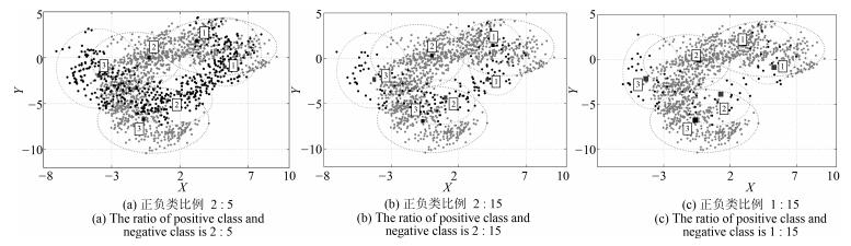 图 5 BFCCL在Banana集上正负类聚类数均为3时的聚类效果Fig. 5 The clustering results on the Banana dataset in BFCCL with three clustering on the positive and negative classes, respectively
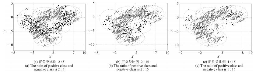 图 6 BFC在Banana集上正负类聚类数均为4时的聚类效果Fig. 6 The clustering results on the Banana dataset in BFC with four clustering on the positive and negative classes, respectively
 图 7 BFCCL在Banana集上正负类聚类数均为4时的聚类效果Fig. 7 The clustering results on the Banana dataset in BFCCL with four clustering on the positive and negative classes, respectively
1) 当在正负两类样本中分别使用BFC算法聚类时, 图 4中(a) ~ (c)中负类样本的聚类效果完全相同, 图 6亦如此.同时在样本重叠区域出现了聚类中心间的距离狭小的现象, 自然由此聚类效果得到的模糊规则的模糊集会存在交叉和重叠的现象.这是因为BFC聚类不考虑不同类别聚类中心间的排斥关系, 运用到模糊系统前件学习中时, 得到的模糊规则其清晰性得不到保证.
2) BFCCL算法考虑了在样本重叠区不同类别聚类中心的竞争关系, 聚类中心由于受到另一个类别样本的排斥而尽量地远离该区域, 这种排斥力最终促使正负类样本的聚类中心尽可能地远离对方样本区域, 从图 5和图 7的聚类效果可知, 随着正类样本数量和分布的变化, 其对负类样本的聚类中心的排斥力的强弱也发生了变化, 负类样本的聚类效果也随之受到了影响.因此在样本重叠区域不会发生聚类中心间的距离狭小的情况.
图 8给出了0-TSK-IDC模糊系统基于图 7(b)聚类结果所获得的模糊集示意图.我们知道, 聚类中心(即模糊规则中心)的分布是决定所获得的模糊规则清晰性和可解释性的决定性因素之一.由图 8可知, BFCCL聚类中的不同类别间聚类中心竞争学习的策略可以保证获得的模糊规则具有良好的可解释性. 表 3为0-TSK-IDC模糊系统中规则前件分别使用BFCCL与BFC算法的性能比较.根据表 3结果可知, 在正负类样本具有不同比例不平衡性的情况下, 与BFC聚类相比, 使用BFCCL聚类获得的解释性强的规则前件参数有助于提高0-TSK-IDC模糊系统的分类性能, 此时$G$-mean和$F$-measure指标均有相应的提高.
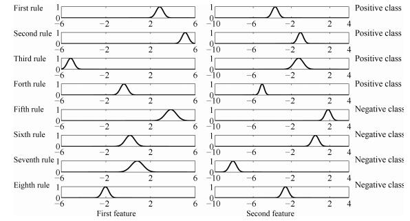 表 3 UCI医学集上分别使用BFCCL与BFC得到规则前件时0-TSK-IDC模糊系统中的G-mean和F-measure值及其方差的比较Table 3 G-mean, F-measure and their standard deviations comparison of 0-TSK-IDC with BFC and BFCCL on UCI datasets
数据集 正负类比例 BFC BFCCL G-mean (%) F-measure (%) G-mean (%) F-measure (%) Heart 12:17 87.01(1.69) 86.87(1.78) 89.56(1.91) 89.36(1.90) 6:17 86.24(2.00) 85.48(1.88) 88.14(1.89) 87.88(1.92) 3:17 85.41(1.97) 84.08(2.00) 87.29(2.01) 86.40(2.00) 2:17 82.50(2.30) 80.02(2.31) 85.71(2.24) 83.63(2.23) 6:85 81.05(2.17) 75.37(2.19) 84.65(2.11) 78.50(2.04) Breast 241:458 93.62(2.60) 91.46(2.57) 96.56(2.34) 95.03(2.20) 100:229 91.14(2.05) 90.02(2.55) 95.59(1.97) 94.24(2.01) 75:229 90.37(2.00) 89.14(2.04) 93.75(1.88) 91.22(1.89) 50:229 87.99(1.90) 85.73(1.89) 91.59(2.03) 89.29(2.10) 20:229 84.21(2.23) 81.26(2.21) 87.56(2.00) 86.05(1.99) Liver 29:40 70.38(0.80) 66.28(0.82) 72.50(0.77) 68.51(0.76) 1:2 69.77(0.75) 61.27(0.75) 71.15(0.69) 62.50(0.60) 1:4 67.82(0.79) 52.98(0.78) 70.24(0.73) 55.22(0.79) Haberman 1:10 65.08(0.81) 47.31(0.83) 67.18(0.75) 50.65(0.72) 9:25 76.05(1.73) 52.75(1.73) 76.56(1.60) 53.61(1.60) 8:45 68.02(1.86) 51.09(1.85) 68.97(1.85) 52.60(1.87) 1:9 64.21(1.69) 48.22(1.73) 65.42(1.74) 50.01(1.69) 4.2.2 真实数据集
为了对BFCCL聚类算法性能作进一步地探讨和分析, 本节使用4个不平衡UCI医学诊断集对BFCCL与BFC算法应用到模糊规则前件参数学习时, 所得的0-TSK-IDC模糊系统的分类性能进行比较. $G$-mean和$F$-measure值及其方差的比较结果如表 3所示.从表 3结果可知, 真实数据集上的实验结果与上一节人工数据集实验上观察到的结果基本保持一致, 在0-TSK-IDC模糊系统中使用BFCCL算法方法后$F$-measure和$G$-mean评价指标均高于使用BFC算法的情况, 说明在使用聚类算法获取模糊规则前件参数的学习中, 充分考虑不同类别聚类中心之间的竞争关系, 有助于提升模糊空间划分的准确性和清晰性.
规则数 正负类比例 BFC BFCCL G-mean (%) F-measure (%) G-mean (%) F-measure (%) 6 2:5 96.48(0.60) 96.2(0.64) 96.97(0.53) 96.44(0.54) 2:15 95.89(0.52) 95.77(0.49) 96.20(0.31) 96.22(0.36) 1:15 94.14(0.47) 93.79(0.41) 95.45(0.55) 94.99(0.48) 8 2:5 97.98(0.31) 97.23(0.34) 99.75(0.27) 99.74(0.23) 2:15 97.03(0.29) 96.92(0.29) 99.32(0.34) 99.32(0.35) 1:15 96.76(0.36) 96.65(0.32) 98.68(0.30) 98.63(0.33) 4.3 0-TSK-IDC模糊分类器与相关分类算法性能比较
为了对0-TSK-IDC模糊分类器的性能进行评估, 本节对0-TSK-IDC与FS-FCSVM、L2-TSK-FS、BFCCL-TSK-FS、Adaboost和CS-SVM五种分类算法进行比较.
4.3.1 人工数据集
本节依旧采用与第4.2.1节相同的Banana数据集进行训练和测试, 表 4列出了6种对比算法的$G$-mean和$F$-measure指标的比较.从实验结果可以看出, 随着Banana数据集中正负类不平衡比例的提高, 6种算法的$F$-measure和$G$-mean指标都呈现出一定的下降趋势, 可见, 数据的不平衡性将严重影响分类的效果.特别是FS-FCSVM、L2-TSK-FS和BFCCL-TSK-FS算法, 由于未考虑类别不平衡性, 当正类样本太少而不能充分学习会导致分类面向正类样本发生了较大的偏移, 其结果是正类样本的分类准确率迅速降低, 因而$G$-mean和$F$-measure指标值也迅速降低.由于充分考虑了不同类别的聚类中心间的竞争学习及数据的不平衡性, 本文提出的0-TSK-IDC模糊系统在分类性能上相比其他5种算法都有提高. CS-SVM算法更多地考虑少数类即正类样本的分类代价, 对正类样本的识别率较高而负类样本的识别率较低; 而Adaboost算法通过过采样技术来增加少数类样本的数量, 由于改变了样本的分布结构容易造成分类器过拟合的情况.因此, 这两种算法获得的$G$-mean和$F$-measure指标值在绝大多数情况下均落后于0-TSK-IDC.
表 4 Banana数据集上0-TSK-IDC模糊分类器与其他算法的G-mean和F-measure值及其方差的比较Table 4 G-mean, F-measure and their standard deviations comparison of 0-TSK-IDC and other algorithms on the Banana dataset正负类样本数 算法 G-mean (%) F-measure (%) 2:5 FS-FCSVM 95.90(0.89) 95.31(0.84) L2-TSK-FS 96.26(0.47) 95.48(0.45) BFCCL-TSK-FS 96.79(0.50) 96.14(0.41) Adaboost 98.77(0.87) 98.71(0.90) CS-SVM 98.98(0.33) 98.91(0.30) 0-TSK-IDC 99.75(0.27) 99.74(0.23) 2:15 FS-FCSVM 90.53(0.65) 89.46(0.60) L2-TSK-FS 89.23(0.71) 88.47(0.72) BFCCL-TSK-FS 92.70(0.58) 92.26(0.62) Adaboost 97.92(0.64) 97.75(0.68) CS-SVM 98.22(0.37) 98.05(0.36) 0-TSK-IDC 99.32(0.34) 99.32(0.35) 1:15 FS-FCSVM 86.06(0.81) 82.83(0.84) L2-TSK-FS 87.95(0.55) 84.67(0.54) BFCCL-TSK-FS 88.84(0.43) 86.33(0.49) Adaboost 97.46(0.58) 97.28(0.52) CS-SVM 97.79(0.74) 97.61(0.70) 0-TSK-IDC 98.68(0.30) 98.63(0.33) 4.3.2 真实数据集
本节给出0-TSK-IDC、FS-FCSVM、BFCCL-TSK-FS、L2-TSK-FS、Adaboost和CS-SVM算法在4个UCI医学诊断数据集上的性能比较, $G$-mean和$F$-measure变化曲线如图 9和图 10所示.从实验结果可以看出,
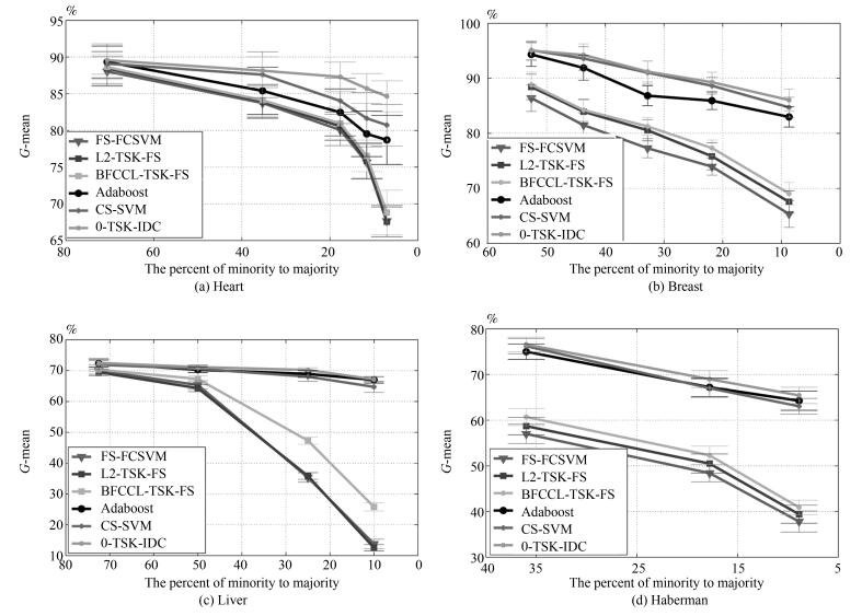 图 9 UCI医学集上不同算法的G-mean比较Fig. 9 G-mean and its standard deviation comparison of 0-TSK-IDC and other algorithms on UCI dataset
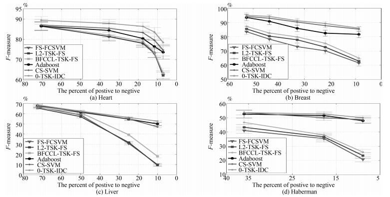 图 10 UCI医学集上不同算法的F-measure比较Fig. 10 F-measure and its standard deviation comparison of 0-TSK-IDC and other algorithms on UCI dataset
1) UCI数据集上获得的实验结果与人工数据集的实验结果是一致的.本文所提的0-TSK-IDC在不同程度的类别不平衡场合均表现出优良的分类性能; 特别对不平衡性较大的数据集, 0-TSK-IDC更能体现其较强的鲁棒性.其原因在于0-TSK-IDC模糊系统前件参数的学习使用了BFCCL聚类, BFCCL聚类通过类别间竞争学习的策略能合理获取不平衡两类上的空间划分, 能保证获得的模糊规则中的模糊集的准确性和可解释性; 0-TSK-IDC模糊系统后件参数的学习从纠正分类面的偏移入手, 最终得到的分类面在达到两类间距离的最大化的同时, 保证少数类到分类面的距离不小于多数类到分类面的距离.
2) 真实数据集上类别间样本数量的不平衡性严重影响算法的分类性能, 如图 9和图 10所示, 随着实验中类别不平衡性的加剧, 三种模糊系统FS-FCSVM、L2-TSK-FS和BFCCL-TSK-FS得到的$G$-mean和$F$-measure值也急剧下降.但由于BFCCL-TSK-FS能够借助BFCCL聚类算法得到准确的空间划分结果, 所以其分类效果要优于FS-FCSVM和L2-TSK-FS, 具体表现为BFCCL-TSK-FS在4个UCI数据集上获得的$G$-mean和$F$-measure值均高于FS-FCSVM和L2-TSK-FS获得的值.
3) Adaboost和CS-SVM算法在$G$-mean和$F$-measure值上得到的结果较为相近, 与FS-FCSVM、L2-TSK-FS和BFCCL-TSK-FS这三种模糊系统相比, 两者具有明显的优势; 但与0-TSK-IDC相比两者的性能略差.值得注意的是, 0-TSK-IDC模糊系统另一个突出优点是其构建的模糊规则具有高度的可解释性, 而这一特性是Adaboost和CS-SVM算法所不具备的.
为了进一步考察在真实数据集上0-TSK-IDC构建的模糊规则的可解释性, 图 11给出了Heart集正负类样本数6 : 17、Breast集正负类样本数75 : 229、Liver正负类样本数1 : 4和Haberman集正负类样本数8 : 45时, $G$-mean指标随规则数变化的曲线.可以看出, 图 9中0-TSK-IDC模糊系统识别率最高时所需的模糊规则数分别是7、12、7和6.模糊系统的特点是建立分类性能和模糊规则数之间的平衡, 通常情况下规则数越少的模糊系统其可解释性越强, 图 11的实验结果可以说明从规则数角度看0-TSK-IDC模糊系统具有高度的可解释性.
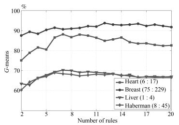 图 11 UCI医学集上G-mean随规则数变化的示意图Fig. 11 G-mean with the different fuzzy rules on UCI databases
5. 结论
本文提出的0-TSK-IDC模糊系统利用BFCCL算法进行模糊规则前件参数的学习, 使基于聚类中心竞争机制和概率模型的聚类算法在类别不平衡的空间划分中表现出了清晰性和可解释性; 0-TSK-IDC模糊系统在模糊规则后件参数的学习中, 使用了"大间隔"的机制并设置少数类到分类面的距离大于多数类到分类面的距离, 从而使得0-TSK-IDC具有较强的泛化能力.本文的主要贡献可以归纳为: 1) 建立一种利用概率模型改进模糊系统的框架; 2) 提出了一种利用聚类模糊系统解决不平衡分类问题的方法.另外, 0-TSK-IDC模糊系统亦可处理类别平衡的分类问题, 只要设置式(23) 和(24) 中参数$v$为0即可.对于多分类问题, 0-TSK-IDC可以采用类似于SVM方法, 用类别组合的方式来实现.应当指出, 本文对0-TSK-IDC模糊系统能否有效解决大样本等问题没有进行深入探讨, 当样本容量极大时, 若从聚类速度和二次规划求解角度而言, 0-TSK-IDC仍面临进一步提高实用性的挑战, 这将作为我们近期的研究重点.
-

图 1 本文深度卷积神经网络的场景重建与语义分类过程
Fig. 1 3D reconstruction and semantic classification of our depth convolutional neural network

图 5 本文摄像头接收范围直接影响网络性能
Fig. 5 Our camera receiving range directly affects performance of network

图 6 带有二进制权值和量化激励的网络层点积分布图. (a), (b), (c), (d)分别为下采样层1、卷积层3、下采样层6、卷积层7的点积分布图(具有不同的均值和标准偏差); (e), (f), (g), (h)分别为下采样层1、卷积层3、下采样层6、卷积层7对应的点积误差分布曲线
Fig. 6 Dot product distribution of network with binary weights and quantitative activation. (a), (b), (c) and (d) are the point product distribution maps of the pooling layer 1, the convolution layer 3, the pooling layer 6 and the convolution layer 7, respectively, they share a different mean and standard deviation; (e), (f), (g) and (h) are the dot product error distribution curves corresponding to the pooling layer 1, the convolution layer 3, the pooling layer 6 and the convolution layer 7, respectively.

图 7 几种复原网络的可视化性能对比图
Fig. 7 Visualization performance comparison for several completion neural networks
表 1 本文网络与L、GW网络的复原与分类性能比较(%)
Table 1 Comparison of three networks for performance of reconstruction and semantic classification (%)
L GW 本文NYU 本文LS_3DDS 本文NYU$+$LS_ 3DDS 复原 闭环率 59.6 66.8 57.0 55.6 69.3 IoU 37.8 46.4 59.1 58.2 58.6 语义场景复原 天花板 0 14.2 17.1 8.8 19.1 地面 15.7 65.5 92.7 85.8 94.6 墙壁 16.7 17.1 28.4 15.6 29.7 窗 15.6 8.7 0 7.4 18.8 椅子 9.4 4.5 15.6 18.9 19.3 床 27.3 46.6 37.1 37.4 53.6 沙发 22.9 25.7 38.0 28.0 47.9 桌子 7.2 9.3 18.0 18.7 19.9 显示器 7.6 7.0 9.8 7.1 12.9 家具 15.6 27.7 28.1 10.4 30.1 物品 2.1 8.3 15.1 6.4 11.6 平均值 18.3 26.8 32.0 27.6 37.3  下载: 导出CSV
表 2 本文网与F网、Z网的重建性能对比数据(%)
Table 2 Comparison of our network reconstruction performance with F and Z networks (%)
训练数据集 复原准确率 闭环率 IoU值 F复原方法 NYU 66.5 69.7 50.8 Z复原方法 NYU 60.1 46.7 34.6 本文复原 NYU 66.3 96.9 64.8 文语义复原 NYU 75.0 92.3 70.3 LS_3DDS 75.0 96.0 73.0
下载: 导出CSV
-
[1] Gupta S, Arbeláez P, Malik J. Perceptual organization and recognition of indoor scenes from RGB-D images. In: Proceedings of 2013 IEEE Conference on Computer Vision and Pattern Recognition (CVPR). Portland, OR, USA: IEEE, 2013. 564-571 http://www.researchgate.net/publication/261227425_Perceptual_Organization_and_Recognition_of_Indoor_Scenes_from_RGB-D_Images [2] Ren X F, Bo L F, Fox D. RGB-(D) scene labeling: features and algorithms. In: Proceedings of 2012 IEEE Conference on Computer Vision and Pattern Recognition (CVPR). Providence, RI, USA: IEEE, 2012. 2759-2766 [3] Silberman N, Hoiem D, Kohli P, Fergus R. Indoor segmentation and support inference from RGBD images. In: Proceedings of the 12th European Conference on Computer Vision. Florence, Italy: Springer, 2012. 746-760 doi: 10.1007/978-3-642-33715-4_54 [4] Lai K, Bo L F, Fox D. Unsupervised feature learning for 3D scene labeling. In: Proceedings of 2014 IEEE International Conference on Robotics and Automation (ICRA). Hong Kong, China: IEEE, 2014. 3050-3057 http://www.researchgate.net/publication/286679738_Unsupervised_feature_learning_for_3D_scene_labeling [5] Rock J, Gupta T, Thorsen J, Gwak J Y, Shin D, Hoiem D. Completing 3D object shape from one depth image. In: Proceedings of 2015 IEEE Conference on Computer Vision and Pattern Recognition (CVPR). Boston, MA, USA: IEEE, 2015. 2484-2493. [6] Shah S A A, Bennamoun M, Boussaid F. Keypoints-based surface representation for 3D modeling and 3D object recognition. Pattern Recognition, 2017, 64:29-38 http://www.wanfangdata.com.cn/details/detail.do?_type=perio&id=0a0d4dd53a9021a3b08eb00743de46f0 [7] Ren C Y, Prisacariu V A, Kähler O, Reid I D, Murray D W. Real-time tracking of single and multiple objects from depth-colour imagery using 3D signed distance functions. International Journal of Computer Vision, 2017, 124(1):80-95 http://www.wanfangdata.com.cn/details/detail.do?_type=perio&id=3e57b7d19aee23e14c99b6a73045ae38 [8] Gupta S, Arbeláez P, Girshick R, Malik J. Aligning 3D models to RGB-D images of cluttered scenes. In: Proceedings of 2015 IEEE Conference on Computer Vision and Pattern Recognition (CVPR). Boston, Massachusetts, USA: IEEE, 2015. 4731-4740 [9] Song S R, Xiao J X. Sliding shapes for 3D object detection in depth images. In: Proceedings of the 13th European Conference on Computer Vision. Zurich, Switzerland: Springer, 2014. 634-651 [10] Li X, Fang M, Zhang J J, Wu J Q. Learning coupled classifiers with RGB images for RGB-D object recognition. Pattern Recognition, 2017, 61:433-446 doi: 10.1016/j.patcog.2016.08.016 [11] Nan L L, Xie K, Sharf A. A search-classify approach for cluttered indoor scene understanding. ACM Transactions on Graphics (TOG), 2012, 31(6): Article No. 137 [12] Lin D H, Fidler S, Urtasun R. Holistic scene understanding for 3D object detection with RGBD cameras. In: Proceedings of 2013 IEEE International Conference on Computer Vision (ICCV). Sydney, NSW, Australia: IEEE, 2013. 1417-1424 [13] Ohn-Bar E, Trivedi M M. Multi-scale volumes for deep object detection and localization. Pattern Recognition, 2017, 61:557-572 doi: 10.1016/j.patcog.2016.06.002 [14] Zheng B, Zhao Y B, Yu J C, Ikeuchi K, Zhu S C. Beyond point clouds: scene understanding by reasoning geometry and physics. In: Proceedings of 2013 IEEE Conference on Computer Vision and Pattern Recognition. Portland, OR, USA: IEEE, 2013. 3127-3134 http://www.researchgate.net/publication/261263632_Beyond_Point_Clouds_Scene_Understanding_by_Reasoning_Geometry_and_Physics [15] Kim B S, Kohli P, Savarese S. 3D scene understanding by voxel-CRF. In: Proceedings of 2013 IEEE International Conference on Computer Vision (ICCV). Sydney, NSW, Australia: IEEE, 2013. 1425-1432 [16] Häne C, Zach C, Cohen A, Angst R. Joint 3D scene reconstruction and class segmentation. In: Proceedings of 2013 IEEE Conference on Computer Vision and Pattern Recognition (CVPR). Portland, OR, USA: IEEE, 2013. 97-104 http://www.researchgate.net/publication/261448707_Joint_3D_Scene_Reconstruction_and_Class_Segmentation [17] Bláha M, Vogel C, Richard A, Wegner J D, Pock T, Schindler K. Large-scale semantic 3D reconstruction: an adaptive multi-resolution model for multi-class volumetric labeling. In: Proceedings of 2016 IEEE Conference on Computer Vision and Pattern Recognition (CVPR). Las Vegas, NV, USA: IEEE, 2016. 3176-3184 [18] Handa A, Patraucean V, Badrinarayanan V, Stent S, Cipolla R. Understanding real world indoor scenes with synthetic data. In: Proceedings of 2016 IEEE Conference on Computer Vision and Pattern Recognition (CVPR). Las Vegas, NV, USA: IEEE, 2016. 4077-4085 [19] 吕朝辉, 沈萦华, 李精华.基于Kinect的深度图像修复方法.吉林大学学报(工学版), 2016, 46(5):1697-1703 http://d.old.wanfangdata.com.cn/Periodical/jlgydxzrkxxb201605046Lv Chao-Hui, Shen Ying-Hua, Li Jing-Hua. Depth map inpainting method based on Kinect sensor. Journal of Jilin University (Engineering and Technology Edition), 2016, 46(5):1697-1703 http://d.old.wanfangdata.com.cn/Periodical/jlgydxzrkxxb201605046 [20] 胡长胜, 詹曙, 吴从中.基于深度特征学习的图像超分辨率重建.自动化学报, 2017, 43(5):814-821 http://www.aas.net.cn/CN/abstract/abstract19059.shtmlHu Chang-Sheng, Zhan Shu, Wu Cong-Zhong. Image super-resolution based on deep learning features. Acta Automatica Sinica, 2017, 43(5):814-821 http://www.aas.net.cn/CN/abstract/abstract19059.shtml [21] Wang P S, Liu Y, Guo Y X, Sun C Y, Tong X. O-CNN: octree-based convolutional neural networks for 3D shape analysis. ACM Transactions on Graphics (TOG), 2017, 36(4): Article No. 72 [22] Yücer K, Sorkine-Hornung A, Wang O, Sorkine-Hornung O. Efficient 3D object segmentation from densely sampled light fields with applications to 3D reconstruction. ACM Transactions on Graphics (TOG), 2016, 35(3): Article No. 22 http://www.researchgate.net/publication/298910150_Efficient_3D_Object_Segmentation_from_Densely_Sampled_Light_Fields_with_Applications_to_3D_Reconstruction [23] Hyvärinen A, Oja E. Independent component analysis:algorithms and applications. Neural Networks, 2000, 13(4-5):411-430 doi: 10.1016/S0893-6080(00)00026-5 [24] Long J, Shelhamer E, Darrell T. Fully convolutional networks for semantic segmentation. In: Proceedings of 2015 IEEE Conference on Computer Vision and Pattern Recognition (CVPR). Boston, MA, USA: IEEE, 2015. 3431-3440 [25] Guo R Q, Zou C H, Hoiem D. Predicting complete 3D models of indoor scenes. arXiv: 1504.02437, 2015. [26] 孙旭, 李晓光, 李嘉锋, 卓力.基于深度学习的图像超分辨率复原研究进展.自动化学报, 2017, 43(5):697-709 http://www.aas.net.cn/CN/abstract/abstract19048.shtmlSun Xu, Li Xiao-Guang, Li Jia-Feng, Zhuo Li. Review on deep learning based image super-resolution restoration algorithms. Acta Automatica Sinica, 2017, 43(5):697-709 http://www.aas.net.cn/CN/abstract/abstract19048.shtml 期刊类型引用(15)
1. 刘影,徐辉. 基于模糊关联的不平衡数据分类算法研究. 齐齐哈尔大学学报(自然科学版). 2023(04): 21-27 .  百度学术
百度学术2. 顾晓清,倪彤光,张聪,戴臣超,王洪元. 结构辨识和参数优化协同学习的概率TSK模糊系统. 自动化学报. 2021(02): 349-362 . 本站查看3. 刘云朋,霍晓丽,刘智超. 基于深度学习的光纤网络异常数据检测算法. 红外与激光工程. 2021(06): 288-293 . 百度学术4. 刘云朋,霍晓丽,刘智超. 基于贝叶斯分区数据挖掘的光纤网络异常分析算法. 红外与激光工程. 2021(08): 295-299 . 百度学术5. 王文君,徐娜. 一种面向光纤网络路径优化的机器学习改进算法. 红外与激光工程. 2021(10): 334-339 . 百度学术6. 宋仪轩,邓赵红,秦斌. 融合模糊推理和流形正则化的特征迁移学习. 计算机科学与探索. 2020(03): 449-459 . 百度学术7. 顾晓清,张聪,倪彤光. 基于随机投影的快速凸包分类器. 控制与决策. 2020(05): 1151-1158 . 百度学术8. 高晓光,王晨凤,邸若海. 一种学习稀疏BN最优结构的改进K均值分块学习算法. 自动化学报. 2020(05): 923-933 . 本站查看9. 邱宁佳,沈卓睿,王辉,王鹏. 通信垃圾文本识别的半监督学习优化算法. 计算机工程与应用. 2020(17): 121-128 . 百度学术10. 韩万兵. 开放式网络非均匀采样数据准确挖掘仿真. 计算机仿真. 2020(08): 337-339+388 . 百度学术11. 王俊,杨茹,程显生. 基于机器学习的云存储数据分段聚类方法仿真. 计算机仿真. 2020(06): 475-478 . 百度学术12. 陈虹,肖越,肖成龙,陈建虎. 融合最大相异系数密度的SMOTE算法的入侵检测方法. 信息网络安全. 2019(03): 61-71 . 百度学术13. 曹雅茜,黄海燕. 基于代价敏感大间隔分布机的不平衡数据分类算法. 华东理工大学学报(自然科学版). 2019(04): 606-613 . 百度学术14. 如先姑力·阿布都热西提,亚森·艾则孜,郭文强. 维语网页中n-gram模型结合类不平衡SVM的不良文本过滤方法. 计算机应用研究. 2019(11): 3410-3414 . 百度学术15. 吴青,张昱,臧博研,祁宗仙. 基于马氏距离的可能性熵聚类算法. 计算机仿真. 2019(12): 240-243+312 . 百度学术其他类型引用(6)
-

 下载:
下载:


计量
- 文章访问数: 1949
- HTML全文浏览量: 413
- PDF下载量: 126
- 被引次数: 21
