

-
摘要: 针对自适应聚类集成选择方法(Adaptive cluster ensemble selection,ACES)存在聚类集体稳定性判定方法不客观和聚类成员选择方法不够合理的问题,提出了一种改进的自适应聚类集成选择方法(Improved ACES,IACES).IACES依据聚类集体的整体平均归一化互信息值判定聚类集体稳定性,若稳定则选择具有较高质量和适中差异性的聚类成员,否则选择质量较高的聚类成员.在多组基准数据集上的实验结果验证了IACES方法的有效性:1)IACES能够准确判定聚类集体的稳定性,而ACES会将某些不稳定的聚类集体误判为稳定;2)与其他聚类成员选择方法相比,根据IACES选择聚类成员进行集成在绝大部分情况下都获得了更佳的聚类结果,在所有数据集上都获得了更优的平均聚类结果.Abstract: Adaptive cluster ensemble selection (ACES) is not only non-objective in judging the stability of cluster ensemble but also unreasonable in selecting cluster members. To overcome such drawbacks, an improved adaptive cluster ensemble selection (IACES) approach is proposed. First, IACES judges the stablity of cluster ensemble according to its total average normalized mutual information. Second, if cluster ensemble is stable, then cluster members with high quality and moderate diversity are selected, else, cluster members with high quality are selected. We evaluate the proposed method on several benchmark datasets and the results show that IACES can judge the stability of cluster ensemble correctedly while ACES misjudges some unstable cluster ensemble as stable. Besides, ensembling the cluster members selected by IACES produces better final solutions than other cluster member selection methods in almost all cases, and is superior average results in all cases.
-
Key words:
- Machine learning /
- cluster analysis /
- cluster ensemble /
- cluster ensemble selection
1) 本文责任编委 赵铁军 -
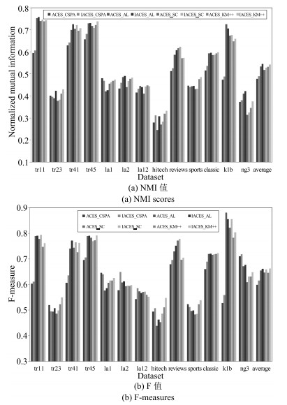
图 2 采用聚类集体P1时获得的聚类结果(NMI值和F值)
Fig. 2 Clustering results obtained when using cluster ensemble P1 (NMI scores and F measures)

图 3 采用聚类集体P2时获得的聚类结果(NMI值和F值)
Fig. 3 Clustering results obtained when using cluster ensemble P2 (NMI scores and F measures)
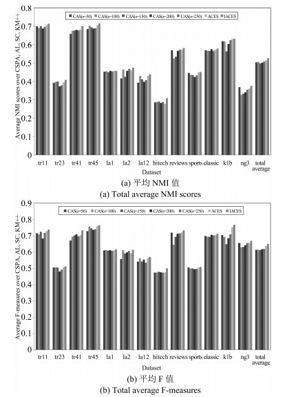
图 4 当采用聚类集体P1时获得的聚类结果(平均NMI值和平均F值)
Fig. 4 Clustering results obtained by combining cluster members selected by ACES and IACES via CSPA, AL, SC and KM++ when using cluster ensemble P1 (Total average NMI scores and total average F measures)
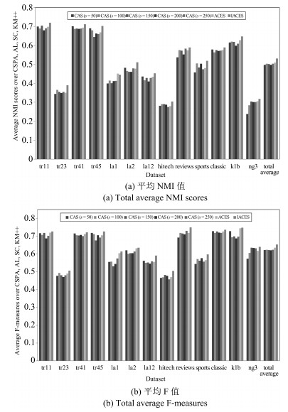
图 5 当采用聚类集体P1时获得的聚类结果(平均NMI值和平均F值)
Fig. 5 Clustering results obtained by combining cluster members selected by ACES and IACES via CSPA, AL, SC and KM++ when using cluster ensemble P1 (Total average NMI scores and total average F measures)
表 1 实验数据集描述
Table 1 Description of datasets
Dataset $n_{d}$ $n_{w}$ $k$$^{\ast }$ $n_{c}$ Balance tr11 414 6 429 9 46 0.046 tr23 204 5 832 6 34 0.066 tr41 878 7 454 10 88 0.037 tr45 690 8 261 10 69 0.088 la1 3 204 31 472 6 534 0.290 la2 3 075 31 472 6 543 0.274 la12 6 279 31 472 6 1 047 0.282 hitech 2 301 10 080 6 384 0.192 reviews 4 069 18 483 5 914 0.098 sports 8 580 14 870 7 1 226 0.036 classic 7 094 41 681 4 1 774 0.323 k1b 2 340 21 839 6 390 0.043 ng3 2 998 15 810 3 999 0.998  下载: 导出CSV
表 2 分别根据ACES和IACES判定的聚类集体稳定性结果
Table 2 Stability results of cluster ensemble according to ACES and IACES
聚类集体$P_{1}$ 聚类集体$P_{2}$ ACES IACES ACES IACES Dataset MNMI Number Stability TANMI Proportion Stability MNMI Number Stability TANMI Proportion Stability tr11 0.655 989 S 0.539 0.7498 S 0.682 940 S 0.574 0.8384 S tr23 0.663 991 S 0.607 0.9361 S 0.712 904 S 0.649 0.8736 S tr41 0.731 999 S 0.642 0.9939 S 0.732 959 S 0.649 0.8922 S tr45 0.718 1 000 S 0.640 0.9917 S 0.705 922 S 0.616 0.8121 S la1 0.597 863 S 0.514 0.5553 S 0.592 894 S 0.541 0.6879 S la2 0.593 934 S 0.524 0.6296 S 0.539 735 S 0.489 0.4374 NS la12 0.634 973 S 0.558 0.7586 S 0.570 838 S 0.493 0.4938 NS hitech 0.551 727 S 0.475 0.3251 NS 0.537 654 S 0.458 0.2602 NS reviews 0.683 940 S 0.610 0.8480 S 0.672 958 S 0.608 0.7622 S sports 0.736 998 S 0.652 0.9637 S 0.651 958 S 0.585 0.7443 S classic 0.801 966 S 0.692 0.8375 S 0.709 945 S 0.594 0.7500 S k1b 0.673 994 S 0.585 0.8992 S 0.654 969 S 0.555 0.7811 S ng3 0.541 664 S 0.451 0.3791 NS 0.525 648 S 0.467 0.4441 NS
下载: 导出CSV
-
[1] Duda R O, Hart P E, Stork D G. Pattern Classification (2nd edition). New York:John Wiley and Sons, 2001. [2] Jain A K, Murty M N, Flynn P J. Data clustering:a review. ACM Computing Surveys (CSUR), 1999, 31(3):264-323 doi: 10.1145/331499.331504 [3] Jain A K. Data clustering:50 years beyond K-means. Pattern Recognition Letters, 2010, 31(8):651-666 doi: 10.1016/j.patrec.2009.09.011 [4] Lee D D, Seung H S. Learning the parts of objects by non-negative matrix factorization. Nature, 1999, 401(6755):788-791 doi: 10.1038/44565 [5] Frey B J, Dueck D. Clustering by passing messages between data points. Science, 2007, 315(5814):972-976 doi: 10.1126/science.1136800 [6] Deng Z H, Choi K S, Jiang Y Z, Wang J, Wang S T. A survey on soft subspace clustering. Information Sciences, 2014, 348:84-106 http://dl.acm.org/citation.cfm?id=2906693 [7] Hinton G E, Salakhutdinov R R. Reducing the dimensionality of data with neural networks. Science, 2006, 313(5786):504-507 doi: 10.1126/science.1127647 [8] Xie J Y, Girshick R, Farhadi A. Unsupervised deep embedding for clustering analysis. In:Proceedings of the 33rd International Conference on Machine Learning. New York City, NY, USA:International Machine Learning Society, 2016. 478-487 [9] Rodriguez A, Laio A. Clustering by fast search and find of density peaks. Science, 2014, 344(6191):1492-1496 doi: 10.1126/science.1242072 [10] von Luxburg U. A tutorial on spectral clustering. Statistics and Computing, 2007, 17(4):395-416 doi: 10.1007/s11222-007-9033-z [11] Strehl A, Ghosh J. Cluster ensembles-a knowledge reuse framework for combining multiple partitions. The Journal of Machine Learning Research, 2002, 3(3):583-617 http://dl.acm.org/citation.cfm?id=944935 [12] Topchy A, Jain A K, Punch W. A mixture model for clustering ensembles. In:Proceedings of the 4th SIAM International Conference on Data Mining. Lake Buena Vista, FL, USA:SIAM, 2004. 379-390 [13] Fern X Z, Brodley C E. Solving cluster ensemble problems by bipartite graph partitioning. In:Proceedings of the 21st International Conference on Machine Learning. Banff, Alberta, Canada:ACM, 2004. 36 [14] Fred A L N, Jain A K. Combining multiple clusterings using evidence accumulation. IEEE Transactions on Pattern Analysis and Machine Intelligence, 2005, 27(6):835-850 doi: 10.1109/TPAMI.2005.113 [15] Li T, Ding C, Jordan M I. Solving consensus and semi-supervised clustering problems using nonnegative matrix factorization. In:Proceedings of the 7th IEEE International Conference on Data Mining (ICDM). Omaha, NE, USA:IEEE, 2007. 577-582 [16] Ayad H G, Kamel M S. Cumulative voting consensus method for partitions with variable number of clusters. IEEE Transactions on Pattern Analysis and Machine Intelligence, 2008, 30(1):160-173 doi: 10.1109/TPAMI.2007.1138 [17] Iam-On N, Boongeon T, Garrett S, Price C. A link-based cluster ensemble approach for categorical data clustering. IEEE Transactions on Knowledge and Data Engineering, 2012, 24(3):413-425 doi: 10.1109/TKDE.2010.268 [18] Carpineto C, Romano G. Consensus clustering based on a new probabilistic rand index with application to subtopic retrieval. IEEE Transactions on Pattern Analysis and Machine Intelligence, 2012, 34(12):2315-2326 doi: 10.1109/TPAMI.2012.80 [19] Wu J J, Liu H F, Xiong H, Cao J, Chen J. K-means-based consensus clustering:a unified view. IEEE Transactions on Knowledge and Data Engineering, 2015, 27(1):155-169 doi: 10.1109/TKDE.2014.2316512 [20] Berikov V, Pestunov I. Ensemble clustering based on weighted co-association matrices:error bound and convergence properties. Pattern Recognition, 2017, 63:427-436 doi: 10.1016/j.patcog.2016.10.017 [21] Zhou Z H, Tang W. Clusterer ensemble. Knowledge-Based Systems, 2006, 19(1):77-83 doi: 10.1016/j.knosys.2005.11.003 [22] Yang Y, Kamel M S. An aggregated clustering approach using multi-ant colonies algorithms. Pattern Recognition, 2006, 39(7):1278-1289 doi: 10.1016/j.patcog.2006.02.012 [23] 罗会兰, 孔繁胜, 李一啸.聚类集成中的差异性度量研究.计算机学报, 2007, 30(8):1315-1324 doi: 10.3321/j.issn:0254-4164.2007.08.013Luo Hui-Lan, Kong Fan-Sheng, Li Yi-Xiao. An analysis of diversity measures in clustering ensembles. Chinese Journal of Computers, 2007, 30(8):1315-1324 doi: 10.3321/j.issn:0254-4164.2007.08.013 [24] Yu Z W, Li L, Liu J M, Zhang J, Han G Q. Adaptive noise immune cluster ensemble using affinity propagation. IEEE Transactions on Knowledge and Data Engineering, 2015, 27(12):3176-3189 doi: 10.1109/TKDE.2015.2453162 [25] 褚睿鸿, 王红军, 杨燕, 李天瑞.基于密度峰值的聚类集成.自动化学报, 2016, 42(9):1401-1412 http://www.aas.net.cn/CN/abstract/abstract18928.shtmlChu Rui-Hong, Wang Hong-Jun, Yang Yan, Li Tian-Rui. Clustering ensemble based on density peaks. Acta Automatica Sinica, 2016, 42(9):1401-1412 http://www.aas.net.cn/CN/abstract/abstract18928.shtml [26] Xu S, Chan K S, Gao J, Xu X F, Li X F, Hua X P, An J. An integrated K-means-Laplacian cluster ensemble approach for document datasets. Neurocomputing, 2016, 214:495-507 doi: 10.1016/j.neucom.2016.06.034 [27] Fern X Z, Lin W. Cluster ensemble selection. Statistical Analysis and Data Mining, 2008, 1(3):128-141 doi: 10.1002/sam.v1:3 [28] Azimi J, Fern X. Adaptive cluster ensemble selection. In:Proceedings of the 21st International Joint Conference on Artificial Intelligence. Pasadena, California, USA:ACM, 2009. 992-997 [29] Naldi M C, Carvalho A C P L F, Campello R J G B. Cluster ensemble selection based on relative validity indexes. Data Mining and Knowledge Discovery, 2013, 27(2):259-289 doi: 10.1007/s10618-012-0290-x [30] 毕凯, 王晓丹, 邢雅琼.基于证据空间有效性指标的聚类选择性集成.通信学报, 2015, 36(8):135-145 http://d.old.wanfangdata.com.cn/Periodical/txxb201508017Bi Kai, Wang Xiao-Dan, Xing Ya-Qiong. Cluster ensemble selection based on validity index in evidence space. Journal on Communications, 2015, 36(8):135-145 http://d.old.wanfangdata.com.cn/Periodical/txxb201508017 [31] Iam-On N, Boongoen T. Comparative study of matrix refinement approaches for ensemble clustering. Machine Learning, 2015, 98(1-2):269-300 doi: 10.1007/s10994-013-5342-y [32] Fern X Z, Brodley C E. Random projection for high dimensional data clustering:a cluster ensemble approach. In:Proceedings of the 20th International Conference on Machine Learning. Washington, DC, USA:ACM, 2003. 186-193 [33] Hadjitodorov S T, Kuncheva L I, Todorova L P. Moderate diversity for better cluster ensembles. Information Fusion, 2006, 7(3):264-275 doi: 10.1016/j.inffus.2005.01.008 [34] Ng A Y, Jordan M I, Weiss Y. On spectral clustering:analysis and an algorithm. In:Proceedings of the 14th International Conference on Neural Information Processing Systems:Natural and Synthetic. Vancouver, British Columbia, Canada:ACM, 2001. 849-856 [35] 徐森, 周天, 于化龙, 李先锋.一种基于矩阵低秩近似的聚类集成算法.电子学报, 2013, 41(6):1219-1224 doi: 10.3969/j.issn.0372-2112.2013.06.028Xu Sen, Zhou Tian, Yu Hua-Long, Li Xian-Feng. Matrix low rank approximation-based cluster ensemble algorithm. Acta Electronica Sinica, 2013, 41(6):1219-1224 doi: 10.3969/j.issn.0372-2112.2013.06.028 [36] 周林, 平西建, 徐森, 张涛.基于谱聚类的聚类集成算法.自动化学报, 2012, 38(8):1335-1342 http://www.aas.net.cn/CN/abstract/abstract17740.shtmlZhou Lin, Ping Xi-Jian, Xu Sen, Zhang Tao. Cluster ensemble based on spectral clustering. Acta Automatica Sinica, 2012, 38(8):1335-1342 http://www.aas.net.cn/CN/abstract/abstract17740.shtml [37] Krogh A, Vedelsby J. Neural network ensembles, cross validation and active learning. In:Proceedings of the 7th International Conference on Neural Information Processing Systems. Denver, CO, USA:ACM, 1994. 231-238 [38] Han E H, Boley D, Gini M, Gross R, Hastings K, Karypis G, Kumar V, Mobasher B, Moore J. WebACE:a web agent for document categorization and exploration. In:Proceedings of the 2nd International Conference on Autonomous Agents. Minneapolis, Minnesota, USA:ACM, 1998. 408-415 -

 下载:
下载:

计量
- 文章访问数: 2534
- HTML全文浏览量: 534
- PDF下载量: 864
- 被引次数: 0
